If you take the annual CO2 atmospheric content, and differentiate it, that is calculate the year-to-year change, then you get a plot that looks a lot like the ocean temperature. This has led many people to think that the ocean is the source of the additional CO2. This is not the case.
The additional CO2 is from about one-half of our emissions. The year-to-year “noise” is from the year-to-year change in ocean temperature riding on the change from our emissions. Changes in our emissions are somewhat filtered by the time constant of CO2 biosphere absorption. Here is what happens.
Many of you will be familiar with the concept of “half-life” from radioactive decay. For a radioactive element, half of the radioactivity will decay in a certain period of time, then half again in the next period, and so on until the radioactivity can no longer be detected. The same principle applies to absorption. Half of a compound will be absorbed in a certain period, then another half in the next period, then another half, and so on. Here is the curve for a pulse of CO2 absorbed into the biosphere.
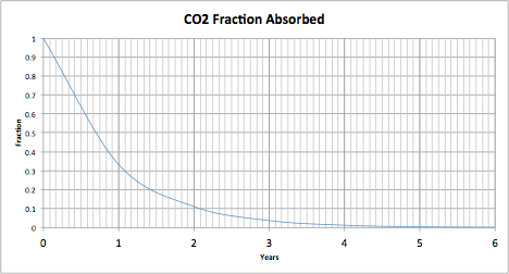
Figure 1 is the absorption curve for a single pulse of CO2 emitted into the atmosphere. The half-life of that pulse is a bit over 8 months. It is undetectable after about six years.
Imagine that you have just taken a deep breath, held it until the maximum CO2 has been exchanged, then exhaled. Half of the CO2 in that puff will be gone from the atmosphere in 8 months, 33% will remain in a year, only 11% will be around in 2 years, and so on. The series is actually 1/3, 1/9, 1/27, 1/81… Now add up all breathing for many years, or all the fossil fuel emissions.
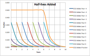
In Figure 2 above the top gold trace is the summation of all the individual annual half-life traces. For instance, year one is the sum of the remainders from year -4 to year zero. It is the sum of 1/243 + 1/81 + 1/27 + 1/9 + 1/3 = very close to 1/2. The CO2 fraction that we observe is close to 0.5. If emissions completely ceased in year six, the extra CO2 added to the atmosphere would be nearly zero in year 10.
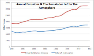
Figure 3 is a plot of annual fossil fuel emissions and the amount of those emissions that annually remain in the atmosphere. The remainder plot has been corrected for half-life.
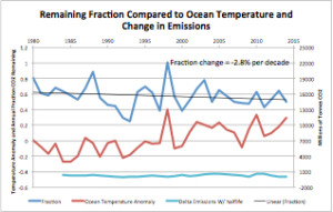
Figure 4 is a plot of the fraction of emissions that remain in the atmosphere, the ocean temperature anomaly (from UHA satellite data), and the change (delta) in emissions with the data corrected for half-life using the fraction change data. (The half-life has been decreasing over time by 2.8% per decade). The left scale is for both the remaining fraction and temperature anomaly. The right scale applies to the delta emissions (the annual change in added emissions). This is scaled to match the fraction change. On a year-to-year basis the ocean temperature changes overwhelm the emission changes, but not the emissions themselves.
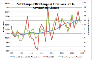
Figure 5 is a plot of change: SST, CO2, and annual emissions added since 1980. This is the annual delta (differential) of all three. The Mt. Pinatubo cooling and the 1998 and 2010 El Niño warming is clearly visible in the CO2 data. It looks like the CO2 increase is due to ocean temperature, but this is an illusion. The annually added emissions are much larger than the ocean temperature CO2 flux change.
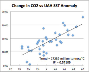
Figure 6 is a scatter plot of CO2 and SST anomaly with a linear trend applied. The trend is 17,239 million metric tonnes of CO2 emitted per degree C of SST change. Now look back at Figure 6. The long term change in temperature is about 0.3°C. This would be equivalent to about 5 billion tonnes of CO2. But the increase in CO2 over that time period was 483 billion tonnes, about 100 times that amount. The long-term CO2 increase is due to emissions, not ocean temperature. Temperature drives only the short-term changes.
About half of fossil carbon emissions appear to be responsible for the atmospheric CO2 rise, and that fraction is decreasing. The year-to-year changes in the CO2 rise are mostly due to ocean temperature changes, but those changes should be considered weather.


I actually agrre with the majority of this post!
Changed your mind then
https://notrickszone.com/2013/03/02/most-of-the-rise-in-co2-likely-comes-from-natural-sources/#sthash.PeRh4gvY.dpbs
So does the trend in the Increase in Atmospheric CO2 equal the Trend in increases in CO2 Emissions?
As I thought the Atmospheric increase was fairly constant whereas Human out put has increased dramatically in the last 25 years.
Yes, I did. I was fooled (along with Dr. Salby) by the similarity of SST and the differential of CO2 rise. It was only when I looked at the amounts of CO2 involved that I realized the flux in and out of the biosphere due to temperature change was much to small to be the cause of CO2 rise.
The trend in increase of CO2 is about half of the trend in emissions. That is reflected in the “remaining fraction”. The remaining fraction gets smaller as more of the human output is taken up. The Atmospheric increase was slow at first, then increased as human output increased.
My comment seems in moderation limbo. Salby is a brilliant man, not a f**l. It is an integral relationship, and it builds over time.
So what you are saying is that the oceans are co² saturated.
They have to be under your hypothesis because if they were not they would absorb at a constant rate with wind stirring noise in the level. Wouldn’t they?
Not saturated, at equilibrium, or very close to it, especially in the “mixed layer” the top 100 meters or so.
Yes, if it was saturated I suppose it would fizz with every movement.
The equilibrium cannot be fixed, somehow it must be an average of the max and min atmospheric atmospheric CO2, so as the atmospheric CO2 increases, so must the equilibrium of the oceans.
This then must reduce the alkalinity of the oceans.
Can this model be validated by the isotope composition of the atmosphere?
Dr. Spencer wrote on that here.
http://wattsupwiththat.com/2008/01/28/spencer-pt2-more-co2-peculiarities-the-c13c12-isotope-ratio/
But, again, the SST signal gets in the way. It’s a good question!
Thanks Ed.
How does this jibe with the IPCC assertion that CO2 remains in the atmosphere for 100 years or more?
Well that’s a completely ludicrous statement by the IPCC.
Seasonal fluctuations of ocean outgassing/absorption.
http://wattsupwiththat.files.wordpress.com/2009/02/eia_co2_contributions_table3.png
production
natural 770000 (Mill t of Gas)
human 23000
absorption 781000
Annual increase 11700
(2001)
Total amount 3.16×10¹⁵ kg = 3.16×10¹² t= 3.16×10^6 Mt= 3.16×10^3 Gt
So, at 3160,000 Mill t total, yearly turnover is about 1/4.5 it seems. So, a 100 years? Whatever they mean with that, they only know themselves.
If emissions suddenly dropped to zero, the CO2 concentration would go down at about the same rate as it went up. The biosphere would take out about 2 ppm/year, decreasing to close to zero in something like a hundred years. In your mind fold the historical rise forward into the future. If emissions stayed right where they are now, the CO2 concentration would reach a max late in this century at something like 475 ppm then slowly decrease to an equilibrium lower than that. That level depends on how the biosphere reacts. I expect emissions to slowly fall from the current level, CO2 max in about 2060 at 450 ppm, then slowly falling to an eventual stability at around 400 ppm in 200 years. There is now way to “compute” this as there are too many variables.
If human emissions dropped to zero tomorrow, the rate of change of CO2 would continue to track temperatures, as it has for at least the past 57 years.
“The long-term CO2 increase is due to emissions, not ocean temperature.”
If true, this is good news, because China et al will be continuing to push life giving CO2 into the atmosphere for a long, long time.
Towards 700+ ppm !
Let the world’s plant life breathe and flourish.
Plants are doing fine, and were at 280 ppm. Increasing atmospheric CO2 for their sake is beyond reckless (and many plants wouldn’t do well in the higher temperatures and changed precipitation patterns.
NO, plants do mediocre at 280ppm. It is borderline CO2 level. It like a human living on stale bread and water.
Plants luv much higher levels and thrive when allowed a reasonable level of plant food and nutrients. And as all greenhouse horticulturalists know, the level is 1000+ ppm
And what higher temperatures?? They haven’t changed by more than a degree for a long, long time.
And yes, plants are starting to do fine, because of the increased atmospheric CO2 levels.
You really need to brush on basic plant biology such as stomata density, transpiration etc etc..
There are literally thousands of papers showing that plant start to grow more strongly as CO2 increases, and are not at all happy below or near 280ppm.
David, just visit a local large greenhouse operation and ask about CO2.
One of my friends owns a very large and thriving greenhouse facility growing all sorts of plants for the food and floral industries. He keeps the CO2 level up above 800ppm for nearly everything he grows.
“Towards 700+ ppm!”
It will not get that high.
See: https://notrickszone.com/2015/03/29/co2-emissions-have-been-flat-for-four-years-what-does-this-mean-for-the-future/
pity. isn’t it 🙁
Shows just how much the biosphere is sucking up, because it NEEDS it.
Someone said that so long as emissions are more than is being absorbed the atmospheric concentration will go up.
The sooner this moronic CO2 hatred comes to an end, the better for all life on Earth.
i still do not understand, why uptake will increase in a linear way, even when CO2 in the atmosphere ist past the maximum.
I do not think that it makes any sense.
pity. isn’t it
Shows just how much the biosphere is sucking up, because it needs it.
Someone said that so long as emissions are more than is being absorbed the atmospheric concentration will go up.
If they start to drop towards the pure survival level of 250-280ppm, the world is going to have great difficulty feeding its populations.
The sooner this childish and un-scientific CO2 hatred comes to an end, the better for all life on Earth.
Your approach is simply too simple. It does not make any sense at all.
This old study shows you, mwaht you have to do to have an educated guess at the real effect of more CO2:
http://news.stanford.edu/pr/02/jasperplots124.html
PS: I am seriously worried about the plants you have at home. Water is plant drink, so they can not have enough it, right???
Spend a few days here, simple one.
http://www.co2science.org/data/plant_growth/plantgrowth.php
I am seriously laughing about what are growing at home, and using too much.
“Here is the curve for a pulse of CO2 absorbed into the biosphere.”
That is a model curve, not an actual observation. But, let’s go with it…
“The series is actually 1/3, 1/9, 1/27, 1/81… Now add up all breathing for many years, or all the fossil fuel emissions.”
I’m sorry, but this is not a legitimate analysis. You cannot extrapolate the fractional remainder of a step response to the fractional remainder of a ramping input (and, CO2 emissions have been ramping up – they didn’t just jump up to their present level and halt). You miss an entire polynomial degree doing that.
We can approximate your decay series based on exponential decay with half life of 8 months. Then, exp(-8/tau) = 0.5, so the time constant tau = 11.5. Each month, we will retain exp(-1/tau) = 0.917 of the previous inventory.
So, we have a series
C(k) = 0.9170*C(k-1) + in(k)
where each step k represents a monthly interval. If you inject a one-time unit pulse, and watch the decay, this gives 8 months, 1 year, 2 years, etc… to be 0.917^[8 12 24] = [0.5000 0.3535 0.1250], so pretty close to your values.
Let’s make in(k) a unit ramping input.
C(k) = 0.9170*C(k-1) + k
The asymptotic response (for k large) is approximately
C(k) = := k/(1-0.917) -133
The cumulative sum, however, is
S(k) = S(k-1) + k = k*(k+1)/2
The virtual accumulated sum S(k) is quadratic in k, while the C(k) series is only linear, just like the input (that’s what a negative feedback does, it makes the output track the form of the input). They diverge substantially over time.
The amount C(k) relative to the virtual accumulation S(k) is not 1/2, it is asymptotically (k/(1-0.917) – 133)/(k*(k+1)/2) or more asymptotically 24/k, which is 1/n for n in years. Within two years, it less than 1/2. In 50 years, it is 0.02. (See actual curve for fraction remaining versus months here).
This is why your mdoel does not work. It does not allow long term tracking of the virtual accumulation at some constant, or even nearly constant, factor. It takes down the resultant curve by a full polynomial degree, resulting in progressive divergence.
“Figure 3 is a plot of annual fossil fuel emissions and the amount of those emissions that annually remain in the atmosphere.”
Again, this is just a model. It is not based on anything but desired outcome.
“Figure 4 is a plot of …”
Another model.
“Figure 6 is a scatter plot of CO2 and SST anomaly with a linear trend applied.”
Again, an inappropriate method of analysis. The sensitivity of CO2 to temperature is not in units of ppmv/degC. It is in units of ppmv/degC/unit-of-time. There is an integral relationship with time.
This plot does indeed show, unequivocally, that human inputs have very little impact on atmospheric CO2. Atmospheric CO2 evolves according to a differential equation
dCO2/dt = k*(T – T0)
i.e., the change in CO2 from one epoch to the next is the integral of an affine function of temperature anomaly. Human inputs are essentially superfluous. If I want to know the atmospheric CO2 at any given time in the last 57 years, all I need is the starting value, and the temperature data to integrate this equation, and I will get a very close result.
It is the nature of negative feedback systems to track the level dictated by boundary conditions, and sharply attenuate disturbances. That is all we are, a small disturbance. There is nothing unusual or exotic about this. The Earth’s CO2 regulatory system shrugs off our puny inputs with barely an acknowledgement, and goes where it wants to go.
BTW, you can fix this to have atmospheric CO2 track emissions, somewhat, with a 1/2 fraction if you extend your decay rate out (a very long way) and basically put half the emissions into the oceans with rapid dynamics. This is what the standard modeling does.
It doesn’t mesh with the observations, though, because CO2 absolutely depends on temperatures to the tune of
dCO2/dt = k*(T – T0)
There is a ramp observable in T, and that ramp must be responsible for the ramp in dCO2/dt. But, emissions also have been ramping up. There is no room for this additional ramp input, because the ramp in dCO2/dt is already accounted for by the temperature relationship.
Ergo, CO2 in the atmosphere is regulated by a feedback system which tracks the above equation, and severely attenuates the emissions input.
The point is that the ramp in Temperature is 100 times too small to account for the ramp in CO2. Only the ramp in emissions is large enough.
That simply isn’t the case. There is a seamless correlation between the temperatures and the rate of change of CO2, from low frequency (the ramp) to high frequency (the variations).
That means a temperature modulated process is driving atmospheric CO2. Human emissions are not temperature modulated, hence they cannot be the dominant driving force.
First, I said a pulse, not a ramping input. That whole bit is intended as an approximation. My point is that only some (about a third) of emissions this year are absorbed this year.
Figures 3 and 4 are calculated from measurements, they are not models. They are based on emissions and CO2. The CO2 is converted to tonnes of CO2. There is no “desired outcome”.
In figure 6 the unit of time is one year.
It’s a bad approximation. If yearly emissions have a ramp in them, then the virtual accumulation of those emissions will be quadratic, yet the output of the process you have described would still be linear. They diverge. Rapidly. Within a few years, they are nowhere near having a 2:1 ratio.
“Figures 3 and 4 are calculated from measurements, they are not models.”
The figure descriptions claim a fraction remaining in the atmosphere. That is supposition. That is imposing a model. There is no reason anything remaining has to have any relationship to emissions at all. If sinks are active, and they are, they can absorb every bit of the emissions, and whatever is left has to be from natural tracking of level imposed by boundary conditions.
This is getting worryingly close to the horrible “mass balance” argument, in which it is argued that, because the rise is less than what we have put in, it has to be due to what we have put in. It does not, and the “mass balance” argument is utterly fatuous.
It’s a bad approximation. Further discussion held up in moderation.
Thank you for the discussion. I hope we have inspired others to take another look at this.
You’ve got to think of it in terms of a dynamic system. Every second, large volumes of CO2 are rising in the upwelling ocean waters. Every second, the same amount has to downwell, or it will accumulate at the surface.
So, it isn’t a matter of having a static tank of water, and heating it up, and getting a bounded outgas to the atmosphere due to the slight temperature dependence of the proportionality factor of Henry’s law. It is a matter of choking off the egress of the constant influx, and thereby getting a persistent buildup accumulating over time.
Ed, what about the time-lag, between temperature and CO2 concentration (as shown in the differential). Does this tell us anything?
The lag is to small and to inconsistent. Using annual averages doesn’t give us enough resolution. I think it is weather.
The lag is a consistent 90 degrees of phase. That means, whenever you see some kind of periodic motion, it will be delayed a quarter cycle between temperature input and CO2 output.
And, 90 deg of phase lag across the spectrum is indicative of an integral relationship. The two go hand in hand.
I don’t see it??
If temperature drives CO2 outgassing, the reservoir of CO2 in the atmosphere serves as an integrator of the amount outgassed.
So the DIFFERENTIAL of atmospheric CO2 concentrations should be possibly Granger-caused by temperature (which is what Beenstein and Reingewertz found).
It is more important that increasing temperature decreases downwelling of CO2, which means that the oceans act as an integrator of the upwelling CO2. The atmosphere responds to the oceanic concentration. So, yes, there is a reservoir acting as an integrating element, but it is the ocean reservoir.
Discussion of the 90 deg phase lag appears held up in moderation.
Yeah sure, that’s another, and the more important reservoir. let’s say it’s like a capacitor with charge moved from one plate to the other and back by a bunch of local temperature and partial pressure differerntial-driven pumps. Like the Bern model only realistic.
If you take a function x(t) = sin((2*pi/T)*t), where t is time and T is the period of oscillation, the derivative is dx/dt = (2*pi/T)*cos((2*pi/T)*t) which, due to trig identities, can be expressed as dx/dt = (2*pi/T)*sin((2*pi/T)*(t+T/4)). So, e.g., x(t) peaks at T/4, 5T/4, 9T/4… but, the derivative peaks T/4 before these times. The derivative induces a lead of a quarter cycle. One quarter cycle is 90 degrees out of 360, so we also commonly say it induces a 90 deg phase lead.
Conversely, integration introduces a 90 degree phase lag. If one integrates dx/dt from above, one gets x(t). So, the derivative operation induces a 90 deg phase lead, and the integral operation introduces a 90 deg phase lag.
As far as temporal leads and lags are concerned, the lead or lag time is period dependent. It is less if the period is smaller, and greater if the period is longer.
See here for a plot of dCO2/dt and dT/dt. I scaled dT/dt and added a trend to aid direct comparison (alternatively, I could have detrended dCO2/dt for the visualization, which might have been clearer).
Look at the variations. In many places, the data go up, and they go down, with varying periods between crossings of the trend line. For a brief time interval containing such variations, you can approximate the function as having a functionally trigonometric shape to it. Generally speaking, the temperature rate of change starts the motion, and 1/4 of the duration of the cycle later, the CO2 rate of change repeats it, i.e., CO2 lags temperature.
Look, for example, between 1995 and 1998. The temperature dT/dt series peaks at the boundaries. dCO2/dt, on the other hand, peaks in about late 1995 and late 1998. If the apparent period of this oscillation is about 3 years, then 1/4 cycle is 3/4 years, and that is the delay.
Look again at about 1971 to 1974. We see that dT/dt again completes a cycle about 3 years in duration, so we expect dCO2/dt to lag by about 3/4 year. And, it does.
Look at about 2004.5 to 2005.5. Here, there is a cycle of about 1 year duration. We expect a smaller time delay of about 1/4 year, and that is what we get.
I know you cannot see it all too clearly in this plot, which was made a long time ago when I first started noticing this relationship, using GISS data, which is not the best. But, you can retrieve the data yourself and verify it for yourself.
As I said, the quarter cycle lag (90 degree phase lag) goes hand in hand with an integration. That is why, when we plot the derivative of CO2 against temperature, it all lines up. The derivative operation induces a 90 degree phase lead. CO2 is lagging by 90 degrees of phase, so when we take the derivative, it advances the CO2 series by 90 degrees, and the derivative matches the temperature series.
OK, I see what you are talking about. Have you considered the seasonality? The fact that CO2 rises in Northern Hemisphere winter and falls in summer? There could be an occasional one year delay for biological and/or weather reasons. The weather in one year setting up the biosphere for an increase or decrease in the next year instead of the current year.
There is always a delay. It is across the board, for low frequencies and high frequencies. It is always 90 deg of phase.
It has to be, or the derivative plot would not match so well, because the derivative, always and at every frequency, induces a 90 deg phase lead.
That says this is no intermittent process, but a smoothly consistent one acting over the long term.