Skeptic Papers 2019 (3)

Climate Model Unreliability/Biases/Errors and the Pause

Tapiador et al., 2019     Uncertainties in modeling persist for large parts of the world, suggesting models still limited to the research realm. … It turns out that both GCMs and RCMs [global/regional climate models] appear still limited to provide practical estimates of the world climates even for present climate conditions.  … The results show that there are significant mismatches between the models and the reference data in, for instance, the case of Europe. …  In Equatorial Africa, the RCMs show a surprising lack of capability. The simulations for the whole continent, which include a different number of models and a different domain, improve very slightly. … These results suggest that both GCMs and the RCMs are still too limited to extract definite estimates of the world climates, even for present climate conditions. Moreover, a closer view of the agreement between modeled and observed precipitation in South and Central America, Asia, Australasia and the Arctic raises serious doubts about whether or not such estimates can be used in practice.

Crawford et al., 2019     We have developed ensembles from 34 CMIP5 GCMs using six diverse approaches, including random forest, support vector regression, neural networks, linear regression, and weighted k-nearest neighbors, and compared the performance of the ensembles with each other and the individual GCMs using a robust set of metrics and nonparametric tests. For temperature, random forest outperforms all other ensembles and the best-performing GCM by a statistically significant margin and is able to simulate temporal and spatial patterns in temperature well. None of the ensembles are able to adequately simulate observed precipitation patterns in the study area, likely due to spatial differences in precipitation drivers in the region, as well as the coarseness of the dataset itself.

Liu et al., 2019     Here we provide an observational assessment of rainfall interactions mechanisms (informed by directional transfer of information entropy) that regulate Sahel rainfall. We quantitatively demonstrate that (1) sea surface temperature over the Gulf of Guinea controls moisture advection and transport to the West Sahel region and (2) strong bidirectional interactions exist between local vegetation dynamics and rainfall patterns. Then we assess the directional interaction patterns from nine state‐of‐the‐art Earth System Models (ESMs). We find that most ESMs are able to represent either the unidirectional control of sea surface temperature on precipitation or the bidirectional interaction between vegetation and precipitation. However, none of the ESMs [System Models] represents both interactive patterns. The GFDL and IPSL‐CM5A‐LR models successfully reproduced observed patterns over ~50% of the West Sahel region but were not accurate in reproducing observed precipitation regional trends or interannual variation. We propose that the directional information transfer is a powerful mechanistic benchmark to assess model fidelity at the process level.

Williams et al., 2019     The hiatus in global warming is manifest in several global datasets in the decadal period 2002–2013. … During the more recent hiatus, lightning observations from the Lightning Imaging Sensor in space show no trend in flash rate. Surface-based, radiosonde-based and satellite-based estimates of global temperature have all been examined to support the veracity of the hiatus in global warming over the time interval of the satellite-based lightning record.

He and Yang, 2019     However, three combined gridded observational datasets, four reanalysis datasets, and most of the CMIP5 models cannot capture extreme precipitation exceeding 150 mm day−1, and all underestimate extreme precipitation frequency. The observed spatial distribution of extreme precipitation exhibits two maximum centers, located over the lower-middle reach of Yangtze River basin and the deep South China region, respectively. Combined gridded observations and JRA-55 capture these two centers, but ERA-Interim, MERRA, and CFSR and almost all CMIP5 models fail to capture them. The percentage of extreme rainfall in the total rainfall amount is generally underestimated by 25%–75% in all CMIP5 models.

Bishop et al., 2019    Atmospheric models forced by observed SSTs and fully coupled models forced by historical anthropogenic forcing do not robustly simulate twentieth-century fall wetting in the SE-Gulf. SST-forced atmospheric models do simulate an intensified anticyclonic low-level circulation around the NASH, but the modeled intensification occurred farther west than observed. CMIP5 analyses suggest an increased likelihood of positive SE-Gulf fall precipitation trends given historical and future GHG forcing. Nevertheless, individual model simulations (both SST forced and fully coupled) only very rarely produce the observed magnitude of the SE-Gulf fall precipitation trend.

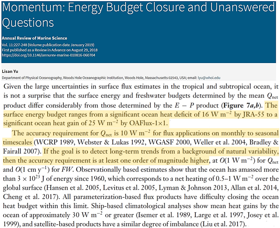
Yu, 2019      Given the large uncertainties in surface flux estimates in the tropical and subtropical ocean, it is not a surprise that the surface energy and freshwater budgets determined by the mean Qnet [energy] product differ considerably from those determined by the E − P product. The surface energy budget ranges from a significant ocean heat deficit of 16 W m−2 by JRA-55 to a significant ocean heat gain of 25 W m−2 by OAFlux-1×1. … The accuracy requirement for Qnet [energy] is 10 W m−2 for flux applications on monthly to seasonal timescales (WCRP 1989, Webster & Lukas 1992, WGASF 2000, Weller et al. 2004, Bradley & Fairall 2007). If the goal is to detect long-term trends from a background of natural variability, then the accuracy requirement is at least one order of magnitude higher, at O(1 W m−2) for Qnet [energy] and O(1 cm y−1) for FW [freshwater]. Observationally based estimates show that the ocean has amassed more than 3 × 1023 J of energy since 1960, which corresponds to a net heating of 0.5–1 W m−2 over the global surface (Hansen et al. 2005, Levitus et al. 2005, Lyman & Johnson 2013, Allan et al. 2014, Cheng et al. 2017). All parameterization-based flux products have difficulty closing the ocean heat budget within this limit. Ship-based climatological analyses show mean heat gains by the ocean of approximately 30 W m−2 or greater (Isemer et al. 1989, Large et al. 1997, Josey et al. 1999), and satellite-based products have a similar degree of imbalance (Liu et al. 2017).

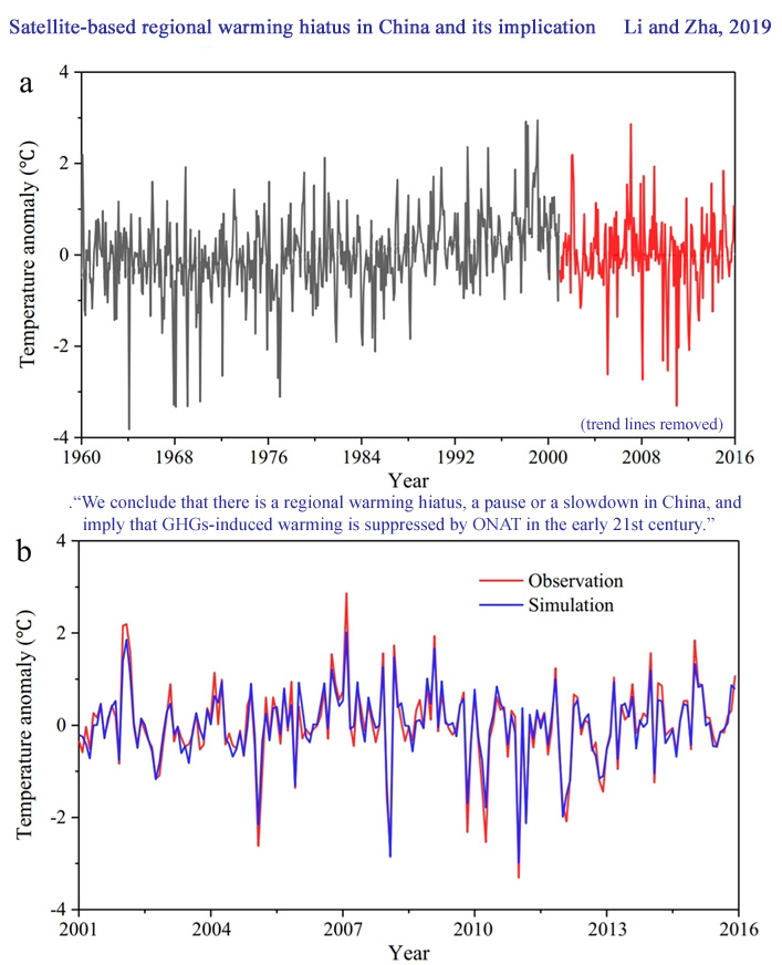
Li et al., 2019     Global warming “stalled” or “paused” for the period 1998–2012, as claimed by the Intergovernmental Panel on Climate Change (IPCC) Fifth Assessment Report (AR5) (IPCC, 2013). However, the early drafts of IPCC AR5 have no detailed explanation for this “hiatus” since 111 of 114 climate models in the CMIP5 earth system model did not verify this phenomenon. … In 2017, after a wave of scientific publications and public debate, the climate models as reported in IPCC remain debates, including definitions of “hiatus” and datasets (Medhaug et al., 2017)…. The slowdown in global warming since 1998, often termed the global warming hiatus. Reconciling the “hiatus” is a main focus in the 2013 climate change conference. Accurately characterizing the spatiotemporal trends in surface air temperature (SAT) is helps to better understand the “hiatus” during the period. This article presents a satellite-based regional warming simulation to diagnose the “hiatus” for 2001–2015 in China. Results show that the rapid warming is mainly in western and southern China, such as Yunnan (mean ± standard deviation: 0.39 ± 0.26 °C (10 yr)−1 ), Tibet (0.22 ± 0.25 °C (10 yr)−1), Taiwan (0.21 ± 0.25 °C (10 yr)−1), and Sichuan (0.19± 0.25 °C (10 yr)−1). On the contrary, there is a cooling trend by 0.29 ± 0.26 °C (10 yr)−1 in northern China during the recent 15 yr, where a warming rate about 0.38 ± 0.11 °C (10 yr)−1 happened for 1960–2000. Overall, satellite simulation shows that the warming rate is reduced to −0.02 °C (10 yr)−1. The changes in underlying surface, Earth’s orbit, solar radiation and atmospheric counter radiation (USEOSRACR) cause China’s temperature rise about 0.02 °C (10 yr)−1. A combination of greenhouse gases (GHGs) and other natural forcing (ONAT, predominately volcanic activity, and atmosphere and ocean circulation) explain another part of temperature trend by approximately −0.04 °C (10 yr)−1. We conclude that there is a regional warming hiatus, a pause or a slowdown in China, and imply that GHGs-induced warming is suppressed by ONAT in the early 21st century.

Williamson and Sansom, 2019   The arguments in this paper make it very clear that strong scientific judgement is implied when linking models to reality, particularly when claiming that a linear relationship between quantities across models indicates a physical relationship. Data mining for constraints may very well lead to a multiple testing problem. A simple numerical experiment can be used to illustrate the point. Generating 430 000 (normal) random numbers and stacking these into a matrix with 43 rows, generates a pseudo ensemble with 43 members and with no physical links between the 10 000 outputs. Looking at the maximum absolute correlation between outputs across the ensemble will usually return correlations between 0.7 and 0.85, well above the threshold for relationships for an emergent constraint. To base the strong beliefs required to take this relationship into the real world (in the way we have made clear), on only the discovery of a large correlation cannot be justified. For that reason, even specifying a low confidence in the constraint through our guided framework would still be inappropriate.

Chen et al., 2019     23 out of the 30 CMIP5 models overestimate the standard deviation of the SLP anomalies north of 20°N. … In particular, 20 out of the 30 models produce stronger SLP anomalies over the North Atlantic (Fig. 4b). By contrast, the CESM1-WACCM and HadGEM2-ES obviously produce a much weaker SLP anomalies over the North Atlantic (Fig. 4b). … The models simulating a stronger spring SLP anomalies over the North Pacifc and North Atlantic do not necessarily have a stronger SLP climatology. Specifcally, the correlation coefficients between the two quantities in Fig. 5a, c are only 0.16 and 0.03, respectively. … Above results suggest that majority of the 30 CMIP5 models cannot realistically reproduce the observed dominant spectral peak of the spring AO index. …  In region B, the MME reproduces weaker positive air temperature anomalies compared to that in the observation (Fig. 10b). This is related to the fact that 26 out of the 30 CMIP5 models simulate a weaker positive ZM air temperature anomaly. …  Out of the 30 models, 28 CMIP5 models produce larger percent variances of the frst EOF mode than that in the observation.

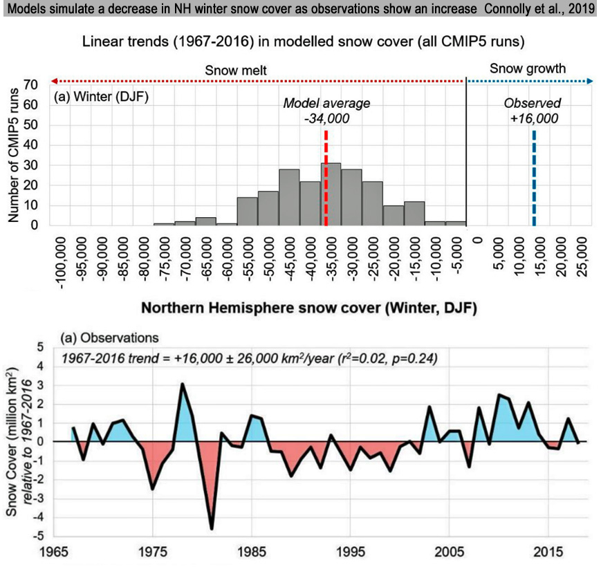
Connolly et al., 2019     Observed changes in Northern Hemisphere snow cover from satellite records were compared to those predicted by all available Coupled Model Intercomparison Project Phase 5 (“CMIP5”) climate models over the duration of the satellite’s records, i.e., 1967–2018. A total of 196 climate model runs were analyzed (taken from 24 climate models). Separate analyses were conducted for the annual averages and for each of the seasons (winter, spring, summer, and autumn/fall). A longer record (1922–2018) for the spring season which combines ground-based measurements with satellite measurements was also compared to the model outputs. The climate models were found to poorly explain the observed trends. While the models suggest snow cover should have steadily decreased for all four seasons, only spring and summer exhibited a long-term decrease, and the pattern of the observed decreases for these seasons was quite different from the modelled predictions. Moreover, the observed trends for autumn and winter suggest a long-term increase, although these trends were not statistically significant.

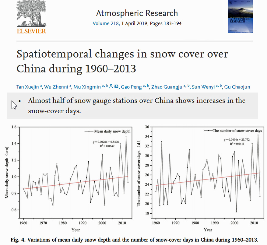
Xuejin et al., 2019     Almost half of snow gauge stations over China shows increases in the snow-cover days.

Seager et al., 2019     State-of-the-art climate models predict that rising GHGs reduce the west-to-east warm-to-cool sea surface temperature gradient across the equatorial Pacific5. In nature, however, the gradient has strengthened in recent decades as GHG concentrations have risen sharply5. This stark discrepancy between models and observations has troubled the climate research community for two decades. … [T]he erroneous warming in state-of-the-art models is a consequence of the cold bias of their equatorial cold tongues. The failure of state-of-the-art models to capture the correct response introduces critical error into their projections of climate change in the many regions sensitive to tropical Pacific sea surface temperatures.

Akhtar, 2019     Many climate scientists have shown disassociation with the IPCC views and speculations on the basis of its doubtful, manipulated, and exaggerated figures of global warming and some consider it a climate scam. [D]ebate between UN pro man-made global warming scientists and anti-man-made global warming climate scientists continue.

Klavans et al., 2019     We cannot reject the null hypothesis that subtropical warming at short lags (0–~4 yr) is a spurious signal introduced by the filter [cf. Fig. 2 herein to Fig. 7 of Delworth et al. (2017)]. Our statistical test does not allow us to conclude that heat anomalies are meridionally advected from the subtropical gyre to the subpolar gyre. Thus, accounting for the influence of the filter, we agree with the literature (e.g., Delworth et al. 2017; Piecuch et al. 2017) that the NAO is associated with a small, lagged, warm response in the subpolar gyre but provides little help in understanding the subtropical or tropical portions of the AMV. … Only 5 of 27 CMIP5 historically forced runs produce a statistically significant lagged warm response to the NAO in the subpolar gyre (Fig. S5). Only 7 of 41 CESM-LE members produce positive lagged warm responses to the NAO in the subpolar gyre (Figs. S6 and S7). … Overall, for only 17 out of 68 historically forced model runs we can reject the null hypothesis that the AMV+ followed the NAO+ by chance. … While this lagged signal appears in some PI control runs, there are large discrepancies between models and observations (Table 1). Observed SSTs warm about 14–15 yr after a NAO+, whereas simulated SSTs warm about 7–10 yr after a NAO+. The zonal mean spatial structure of the response in observations appears to be very different from most CMIP5 models.

Eyring et al., 2019     Despite substantial progress in climate modelling over the past few decades, there remains a substantial spread in projections of future climate change. For example, the range of model estimates for ECS to a doubling of CO2 concentrations has not decreased since the 1970s … There is enough evidence now that the continued assumption of model democracy cannot be fully justified in future IPCC assessment reports. It is not yet clear, however, whether all variables of interest can be reliably constrained.

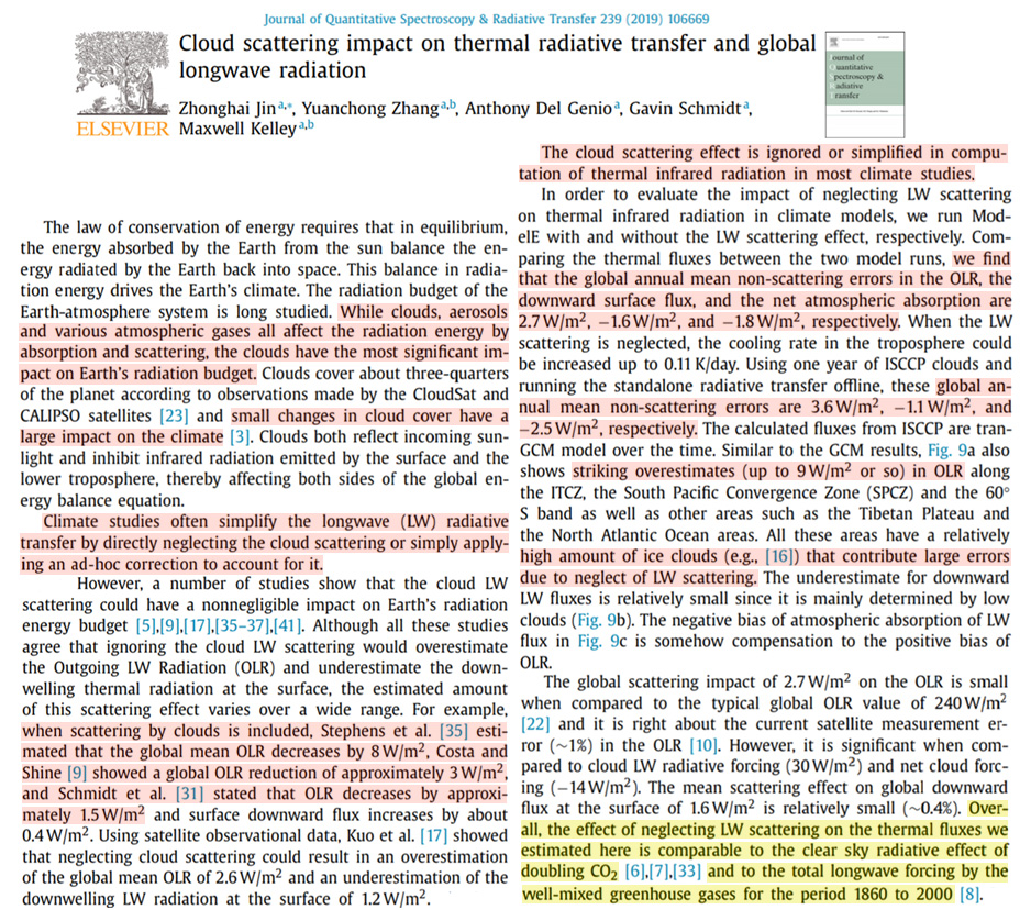
Jin et al., 2019     The radiation budget of the Earth-atmosphere system is long studied. While clouds, aerosols and various atmospheric gases all affect the radiation energy by absorption and scattering, the clouds have the most significant impact on Earth’s radiation budget. Clouds cover about three-quarters of the planet according to observations made by the CloudSat and CALIPSO satellites [23] and small changes in cloud cover have a large impact on the climate [3]. … Climate studies often simplify the longwave (LW) radiative transfer by directly neglecting the cloud scattering or simply applying an ad-hoc correction to account for it. … [A] number of studies show that the cloud LW scattering could have a nonnegligible impact on Earth’s radiation energy budget [5],[9],[17],[35–37],[41]. Although all these studies agree that ignoring the cloud LW scattering would overestimate the Outgoing LW Radiation (OLR) and underestimate the downwelling thermal radiation at the surface, the estimated amount of this scattering effect varies over a wide range. For example, when scattering by clouds is included, Stephens et al. [35] estimated that the global mean OLR decreases by 8W/m², Costa and Shine [9] showed a global OLR reduction of approximately 3W/m², and Schmidt et al. [31] stated that OLR decreases by approximately 1.5W/m² and surface downward flux increases by about 0.4W/m2. … The results show that the change in the OLR has a high anticorrelation (−0.764) with the change in the total cloudiness, while the atmospheric absorption is positively correlated (0.632) with the total cloudiness. … Using one year of ISCCP clouds and running the standalone radiative transfer offline, these global annual mean non-scattering errors are 3.6W/m2, −1.1W/m2, and −2.5W/m2, respectively. … Overall, the effect of neglecting LW scattering on the thermal fluxes we estimated here is comparable to the clear sky radiative effect of doubling CO2 [6],[7],[33] and to the total longwave forcing by the well-mixed greenhouse gases for the period 1860 to 2000 [8].

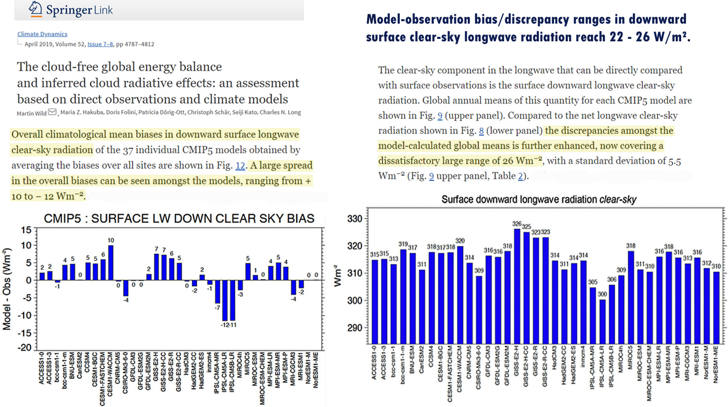
Wild et al., 2019     The clear-sky component in the longwave that can be directly compared with surface observations is the surface downward longwave clear-sky radiation. Global annual means of this quantity for each CMIP5 model are shown in Fig. 9 (upper panel). Compared to the net longwave clear-sky radiation shown in Fig. 8 (lower panel) the discrepancies amongst the model-calculated global means is further enhanced, now covering a dissatisfactory large range of 26 Wm−2, with a standard deviation of 5.5 Wm−2. … Overall climatological mean biases in downward surface longwave clear-sky radiation of the 37 individual CMIP5 models obtained by averaging the biases over all sites are shown in Fig. 12. A large spread in the overall biases can be seen amongst the models, ranging from + 10 to − 12 Wm−2. As with the shortwave biases presented in Fig. 6, this large spread is not surprising, considering the substantial differences amongst the global mean downward surface longwave clear-sky radiation of the various models.

Mehta et al., 2019     Climate-related uncertainty refers to the inability to predict the scale, intensity, and impact of climate change on human and natural environments. Debates of uncertainty in climate change have emerged as a ‘super wicked’ problem for scientists and policy makers alike.

Zhang et al., 2019     A total of 39 out of 48 GCM [general circulation models] SSR [surface incident solar radiation] simulations show an underestimation tendency compared with ground measurements in summer (JJA). The possible reason may be that the GCMs have difficulties in capturing the insulating effect of clouds, since cloud properties represented by GCM SSR estimation models are one of the most important factors in regulating the estimated SSR. … Only slightly more than half of the GCMs (26 out of the 48 GCMs) overestimated the SSR over high-latitude areas when compared with the ground observations, although some discrepancies between the current GCM SSR simulations and ground measurements still existed over high-latitude areas. Cloud and aerosol properties represented by the GCMs are two important factors in regulating the estimated SSR [9]. The GCMs have been reported to overestimate aerosol optical thickness [48] and total cloud cover over high-latitude areas [9,36,47]. … Besides cloud and aerosols, measurement errors, such as instrument replacement and drift and spatial representativeness of ground measurements were also potential error sources of SSR evaluations. For example, the monthly representation errors at the surface sites with respect to their 1° surroundings are on average 3.7% (4 W m−2) [49].

Huang et al., 2019    Realistically representing the Arctic amplification in global climate models (GCMs) represents a key to accurately predict the climate system’s response to increasing anthropogenic forcings. We examined the amplified Arctic warming over the past century simulated by 36 state‐of‐the‐art GCMs against observation. We found a clear difference between the simulations and the observation in terms of the evolution of the secular warming rates. The observed rates of the secular Arctic warming increase from 0.14°C/10a in the early 1890s to 0.21°C/10a in the mid‐2010s, while the GCMs show a negligible trend to 0.35°C/10a at the corresponding times. The overestimation of the secular warming rate in the GCMs starts from the mid‐20th century and aggravates with time. Further analysis indicates that the overestimation mainly comes from the exaggerated heating contribution from the Arctic sea ice melting. This result implies that the future secular Arctic warming may have been over‐projected.

Bryan et al., 2019     Climate model simulations of the summer South Asian monsoon predict increased rainfall in response to anthropogenic warming. However, instrumental data show a decline in Indian rainfall in recent decades, underscoring the critical need for additional, independent records of past monsoon variability.

Scafetta, 2019     GCMs [General Circulation Models] fail to properly reconstruct the natural variability of the climate throughout the entire Holocene and at multiple time scales such as: (1) the Holocene Climatic Optimum (9000-6000 years ago) with the subsequent cooling from 5000 years ago to now; (2) the large millennial oscillations observed throughout the Holocene that were responsible, for example, for the Medieval Warm Period; (3) several shorter climatic oscillations with periods of about 9.1, 10.4, 20, 60 years; (4) the climate change trend after 2000 to date, which the models greatly overestimate; and many other patterns. These different pieces of evidence imply two main facts: (1) the models’ equilibrium climate sensitivity (ECS) to radiative forcing, such as to an atmospheric CO2 doubling, is overestimated at least by a factor of 2, which implies a more realistic ECS between 1°C and 2°C; (2) there are a number of solar and astronomical forcings that are still missing in the models or are poorly understood yet. Consequently, these GCMs are not physically reliable for properly interpreting past and future climatic changes.

Libardoni et al., 2019     Because models are approximations of the real world, we cannot assume that any model will exactly simulate the internal variability of the natural world. Model developers make different decisions when choosing dynamical cores, cloud microphysics schemes, and many other components. These choices impact model behavior, leading to structural uncertainty in the estimation of the patterns of internal variability. Drawing samples from a single model cannot account for this structural uncertainty and leads to only one of the many possible representations being used when estimating covariance matrices. Using multiple models to estimate the internal variability draws samples across the different model structures and better represents the uncertainty we have in knowing the variability of the natural world.

Hofer et al., 2019     Recently, the Greenland Ice Sheet (GrIS) has become the main source of barystatic sea-level rise. The increase in the GrIS melt is linked to anticyclonic circulation anomalies, a reduction in cloud cover and enhanced warm-air advection. The Climate Model Intercomparison Project fifth phase (CMIP5) General Circulation Models (GCMs) do not capture recent circulation dynamics; therefore, regional climate models (RCMs) driven by GCMs still show significant uncertainties in future GrIS sea-level contribution, even within one emission scenario. … The discrepancies between modelled cloud properties within a high-emission scenario introduce larger uncertainties in projected melt volumes than the difference in melt between low- and high-emission scenarios.

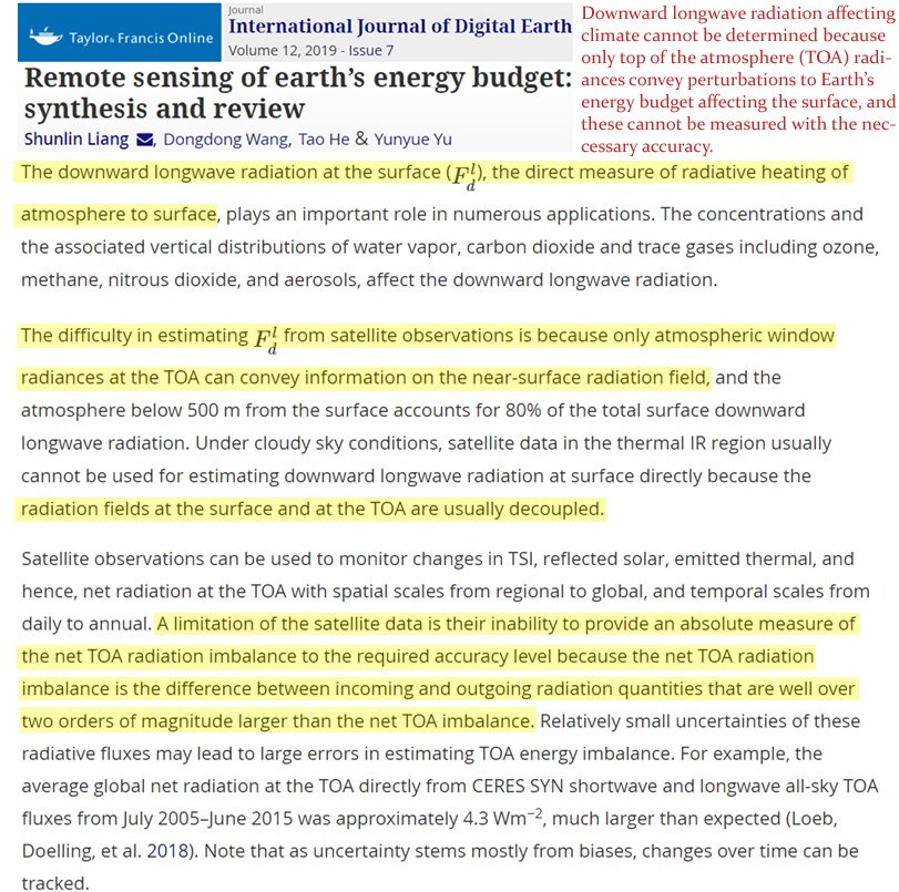
Liang et al., 2019     Significant progress in estimating EEB [Earth’s energy balance] from satellite observations has been made in the past half century, but satellite estimation of EEB still has large uncertainties. For example, most recent studies expect the TOA energy imbalance to be within 0.5–1 Wm−2. Satellite estimation of EEB is based on three individual radiative fluxes (incident solar, reflected shortwave and emitted longwave radiation). As these fluxes are of the order of hundreds of Wm−2, their difference, characterizing the energy imbalance, is too small to be estimated accurately so that the accuracy of 0.1 Wm−2 required by the GCOS (GCOS 2016) would be difficult to meet. The radiometric calibration errors of the satellite sensors also make it impossible to estimate the residual accurately.

Urban Heat Island: Raising Surface Temperatures Artificially

Wen-qian et al., 2019     Based on an in-homogeneity adjusted dataset of the monthly mean temperature, minimum and maximum temperature, this paper analyzes the temporal characteristics of Urban Heat Island (UHI) intensity at Wuhan Station, and its impact on the long-term trend of surface air temperature change recorded during 1961-2015 by using an urban-rural method. Results show that UHI effect is obvious near Wuhan Station in the past 55 years, especially for minimum temperature. The strongest UHI intensity occurs in summer and the weakest in winter. For the period 1961-2004, UHI intensity undergoes a significant increase near the urban station, with the increase especially large for the period 1988-2004, but a significant decrease is registered for the last 10 years, with the decrease in minimum temperature more significant than that of maximum temperature. The annual mean urban warming and its contribution to overall warming are 0.18°C/10yr and 48.8% respectively for the period 1961-2015, with a more significant and larger urbanization effect seen in Tmin than Tmax. A large proportion warming, about half of the overall increase in annual mean temperature, as observed at the urban station, thus can be attributed to the rapid urbanization in the past half a century. … Zhou et al.[9] found that the contribution of urban warming to the overall warming in the northern China region was 37.9% during 1961-2000, and it even reaches 71% at Beijing station over the same period (Chu et al.[17]); Urbanization-induced SAT trend reaches 0.19°C/10yr during 1962-2009 for Shijiazhuang station, accounting for 68% of all warming trend (Bian et al.[18]). … Chen et al.[20] studied the UHI change trend for Wuhan station from 1960 to 2005, and found that the annual mean urban warming and contribution rate reached 0.235°C/10yr and 60.4% respectively.

Yao et al., 2019     In this study, Moderate resolution imaging spectroradiometer (MODIS) land cover, land surface temperature (LST) and enhanced vegetation index (EVI) data were used to investigate the trends of surface urban heat island intensity (SUHII, urban LST minus rural LST) and their relations with vegetation in 397 global big cities during 2001–2017. Major findings include: (1) annual daytime and nighttime SUHII [surface urban heat island intensity] increased significantly (p < 0.05, Mann-Kendall trend test) in 42.1% and 30.5% cities, respectively; (2) the daytime SUHII in the growing season was significantly and positively correlated with rural EVI in 58.9% cities. … Surface urban heat island (SUHI) refers to higher land surface temperature (LST) in urban than in rural areas. The increased SUHI intensity (SUHII, urban LST minus rural) was mainly attributed to increased anthropogenic heat emission and built-up areas, and reductions in vegetation in urban areas in the literature. However, this study showed that the increased vegetation (i.e. greening) in rural areas was a significant and widespread driver for the increased daytime SUHII around the world during 2001–2017.

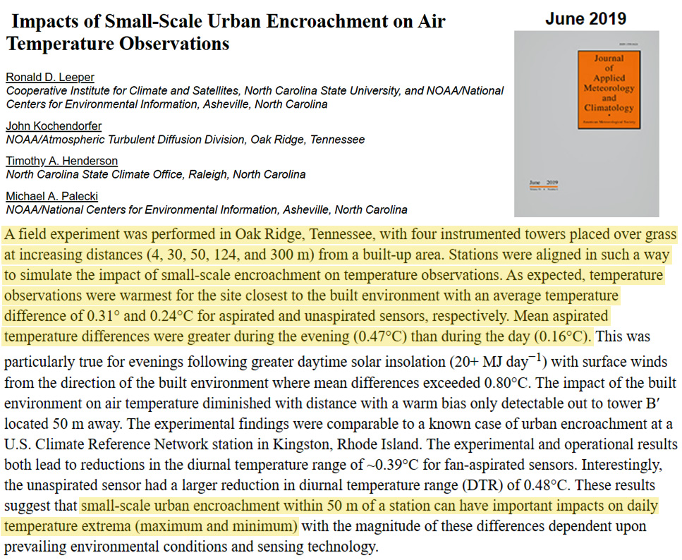
Leeper et al., 2019     These results suggest that small-scale urban encroachment within 50 meters of a station can have important impacts on daily temperature extrema (maximum and minimum) with the magnitude of these differences dependent upon prevailing environmental conditions and sensing technology. … As expected, temperature observations were warmest for the site closest to the built environment with an average temperature difference of 0.31 and 0.24 °C for aspirated and unaspirated sensors respectively. Mean aspirated temperature differences were greater during the evening (0.47 °C) than day (0.16 °C).

Goddard and Tett, 2019     This study aims to estimate the affect of urbanisation on daily maximum and minimum temperatures in the United Kingdom. … For an urban fraction of 1.0, the daily minimum 2‐m temperature was estimated to increase by 1.90 ± 0.88 K while the daily maximum temperature was not significantly affected by urbanisation. This result was then applied to the whole United Kingdom with a maximum T min urban heat island intensity (UHII) of about 1.7K in London and with many UK cities having T min UHIIs above one degree. … This paper finds through the method of observation minus reanalysis that urbanisation has significantly increased the daily minimum 2‐m temperature in the United Kingdom by up to 1.70 K. … Yan et al. (2010) concluded a large impact of urbanisation up to 0.54 K/decade on local temperature series in Beijing.

Gehrig et al., 2019     The goal of the study was to provide a climatological overview of the intensity of the UHI in five main Swiss cities with more than 130’000 inhabitants.The UHI was studied by comparing data series of weather stations located in city centres with weather stations in the rural vicinity. The UHI is calculated as temperature difference between the urban and the rural station. … The UHI is present in all investigated cities during the whole year. Maxima are reached in summer, especially at night. Night temperatures in city centres are on average over 2 K higher in summer than in rural areas. In less densely built-up areas they are between 1 and 2 K higher. Nighttime city temperatures can be up to 6-7 K higher than in rural areas in the vicinity. During the warmest nights, the temperature in the city centres does not drop below 24-25 °C. The number of tropical nights in cities is significantly higher than in rural areas, while the number of hot days is only slightly higher. An exception to this are the monitoring stations in Basel, where the number of hot days is also significantly higher. They represent locations in the immediate vicinity of asphalt and buildings, which warm up strongly during the day.

Shi et al., 2019     Although urban areas constitute less than 1% of land in China, more than 90% of the meteorological stations experienced urban land use change and the average urban expansion rate was 0.33%/a. There was also a significant positive relationship between observed warming trends and urban expansion rates. Background warming, without the influence of urbanization and extra warming induced by urbanization processes, was estimated using a linear regression model based on observed warming trends and urban expansion rates. On average, urbanization led to an additional annual warming of 0.034 ± 0.005 °C/10a. This urbanization warming effect was 0.050 ± 0.007 °C/10a for minimum temperatures and 0.008 ± 0.004 °C/10a for maximum temperatures. Moreover, it appeared that urbanization induced greater warming on the minimum temperature during the cold season and maximum temperature during the warm season.

Scafetta and Ouyang, 2019     A comparison versus China urbanization records demonstrates that the regions characterized by a large Tmin-Tmax divergence are also the most densely populated ones, such as north-east China, that have experienced a diffused and fast urbanization since the 1940s. The results are significant and may indicate the presence of a substantial uncorrected urbanization bias in the Chinese climate records. Under the hypothesis that Tmax is a better metric for studying climatic changes than Tmean or Tmin, we conclude that about 50% of the recorded warming of China since the 1940s could be due to uncorrected urbanization bias. In addition, we also find that the Tmax record from May to October over China shows the 1940s and the 2000s equally warm, in contrast to the 1 °C warming predicted by the CMIP5 models.

Ünal et al., 2019     Land surface data from Moderate-Resolution Imaging Spectroradiometer (MODIS) Aqua and Terra show areal extension of the UHI through the north along the Bosphorus between 2000 and 2012, especially in the night observations. The continuous increase of built-up areas, paved roads, and decrease of green areas caused the growth of UHI intensity. The estimated UHI based on land surface temperature (LST) at the most urbanized locations of Istanbul reach to 8 °C for daytime and 6 °C for nighttime.

Failing Renewable Energy, Climate Policies

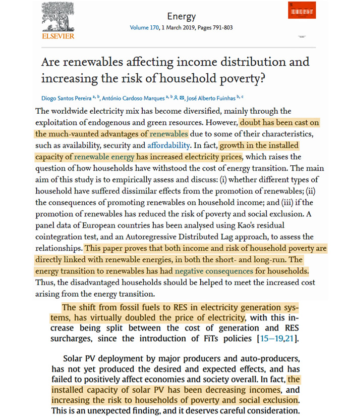
Pereira et al., 2019   [D]oubt has been cast on the much-vaunted advantages of renewables due to some of their characteristics, such as availability, security and affordability. In fact, growth in the installed capacity of renewable energy has increased electricity prices, which raises the question of how households have withstood the cost of energy transition. This paper proves that both income and risk of household poverty are directly linked with renewable energies, in both the short- and long-run. The energy transition to renewables has had negative consequences for households. … The shift from fossil fuels to RES [renewable energy sources] in electricity generation systems, has virtually doubled the price of electricity, with this increase being split between the cost of generation and RES surcharges.

Pendrill et al., 2019     In total, the share of deforestation attributed to exports was greatest for crops (40%), with some—palm oil, soybeans, tree nuts and other crops—primarily destined for export (63–77%). … The largest export flows went from early- and latet-ransition countries to post-transition countries, and the exported deforestation from pretransition countries was primarily consumed in post-transition countries in Europe.

Pendrill et al., 2019     Deforestation, the second largest source of anthropogenic greenhouse gas emissions, is largely driven by expanding forestry and agriculture. …. Similarly, deforestation emissions constitute a substantial share (˜15%) of the total carbon footprint of food consumption in EU countries. This highlights the need for consumption-based accounts to include emissions from deforestation, and for the implementation of policy measures that cross these international supply-chains if deforestation emissions are to be effectively reduced.

(press release)      A sixth of all emissions resulting from the typical diet of an EU citizen can be directly linked to deforestation of tropical forests.  “In effect, you could say that the EU imports large amounts of deforestation every year. If the EU really wants to achieve its climate goals, it must set harder environmental demands on those who export food to the EU,” says Martin Persson from Chalmers, one of the researchers behind the studies. The studies indicate that, although there is a big variation between different EU countries, on average a sixth of the emissions from a typical EU diet can be directly traced back to deforestation in the tropics. Emissions from imports are also high when compared with domestic agricultural emissions. For several EU countries, import emissions connected to deforestation are equivalent to more than half of the emissions from their own, national agricultural production.

Greenstone and Nath, 2019     [R]enewable power plants require ample physical space, are often geographically dispersed, and are frequently located away from population centers, all of which raises transmission costs above those of fossil fuel plants. … [REM-driven] increases in renewable energy penetration can also raise total energy system costs by prematurely displacing existing productive capacity, especially in a period of flat or declining electricity consumption. Adding new renewable installations, along with associated flexibly dispatchable capacity, to a mature grid infrastructure may create a glut of installed capacity that renders some existing baseload generation unnecessary. The costs of these ‘stranded assets’ do not disappear and are borne by some combination of distribution companies, generators, and ratepayers. Thus, the early retirement or decreased utilization of such plants can cause retail electricity rates to rise even while near zero marginal cost renewables are pushing down prices in the wholesale market. … Intermittent wind and solar cannot stand on their own. They must have some form of back-up power, from reliable coal, natural gas, nuclear units, storage capability from hydroelectric facilities, and/or batteries. Batteries of the size and scope needed for 100-percent renewables are unproven and not cost effective. Even if a 100 percent renewable future were feasible, the land requirements and costs of transitioning would be enormous and would require subsidies to ease the electricity price increases that would result.

Nathaniel and Iheonu, 2019     We examined the role of renewable and non-renewable energy consumption on CO2 emissions in Africa. … Renewable energy inhibits CO2 emissions insignificantly in Africa.

Padoan et al., 2019     The rapid increase in the photovoltaic power installed worldwide will cause over the next few decades a dramatic increase in the volume of end-of-life photovoltaic panels. In accordance with the analysis presented in this article, peaks for dismissal of PV panels are expected to occur around the years 2036 and 2045. The improper disposal of these waste fluxes could cause harmful effects to human health and to economy of the manufacture sector by the dispersion of toxic elements and loss of valuable material resources including rare metals, respectively.

Liu et al., 2019     Over the past three decades, China has witnessed spectacular economic growth. However, behind this economic success, the country also faces serious challenges, including pressures to reduce emissions and to address imbalances in its growth. Increasing attention is thus being paid to the task of exploring the relationship between income inequality and CO2 emissions. … China’s energy consumption is dominated by coal, which accounted for 63.7% of the country’s total energy consumption in 2015—China is responsible for more than 50% of the world’s coal consumption. By 2030, China’s CO2 emissions will be equivalent to the rest of the world’s total emissions. … [W]e investigated how the level of income distribution within 30 Chinese provinces influenced that province’s CO2 emissions, using panel data from 1996 to 2014 to estimate both the Gini coefficient and Global Moran’s I. The empirical results show that income growth increased China’s CO2 emissions during the study period, but that an inverted U-shaped relationship existed between income and emissions, thereby confirming the Environmental Kuznets Curve hypothesis. The continuously widening income gap, and especially the uneven spatial distribution of income, can thus be expected to deteriorate environmental quality and increase CO2 emissions. The effect of the self-reinforcing agglomeration of income on emissions was clearly evident.

Marques et al., 2019     CO2 emissions constitute a strong incentive to invest in wind power, but not in solar PV sources. In fact, wind power has mostly been implemented by major players, pressured by political guidelines to reduce CO2 emissions and meet the targets imposed by international commitments (International Energy Agency, 2016). Furthermore, wind power is capable of generating electricity at any time of the day, as well as during the winter and summer seasons. In contrast, solar PV has mainly been deployed on a smaller-scale, and by smaller local players, without political pressure. This has meant that PV still represents a negligible percentage of installed electricity capacity. Consequently, this source has not yet been able to exert the desired effect on reducing carbon dioxide emissions. One might imagine that, if everything remains the same, this effect will persist in the future. However, this negative effect could be reversed in the near future if, along with the decreasing prices of solar PV technology, public policies intervene to incentivize/foster the large-scale implementation of solar PV. Furthermore, rising gross domestic product has the capability of increasing the implementation of solar PV in the long-run, mainly in EU and OECD countries.

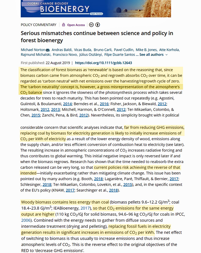
Norton et al., 2019     The classification of forest biomass as ‘renewable’ is based on the reasoning that, since biomass carbon came from atmospheric CO2 and regrowth absorbs CO2 over time, it can be regarded as ‘carbon neutral’ with net emissions over the harvesting/regrowth cycle of zero. The ‘carbon neutrality’ concept is, however, a gross misrepresentation of the atmosphere’s CO2 balance since it ignores the slowness of the photosynthesis process which takes several decades for trees to reach maturity. This has been pointed out repeatedly (e.g. Agostini, Guiintoli, & Boulamanti, 2014; Berndes et al., 2016; Fisher, Jackson, & Biewald, 2012; Holtsmark, 2012, 2013; Mitchell, Harmon, & O’Connell, 2012; Ter‐Mikaelian, Colombo, & Chen, 2015; Zanchi, Pena, & Bird, 2012). … It is thus of considerable concern that scientific analyses indicate that, far from reducing GHG emissions, replacing coal by biomass for electricity generation is likely to initially increase emissions of CO2 per kWh of electricity as a result of the lower energy density of wood, emissions along the supply chain, and/or less efficient conversion of combustion heat to electricity (see later). The resulting increase in atmospheric concentrations of CO2 increases radiative forcing and thus contributes to global warming. This initial negative impact is only reversed later if and when the biomass regrows. Research has shown that the time needed to reabsorb the extra carbon released can be very long, so that current policies risk achieving the reverse of that intended—initially exacerbating rather than mitigating climate change. … Woody biomass contains less energy than coal (biomass pellets 9.6–12.2 GJ/m³; coal 18.4–23.8 GJ/m³; IEABioenergy, 2017), so that CO₂ emissions for the same energy output are higher (110 kg CO₂/GJ for solid biomass, 94.6–96 kg CO₂/GJ for coals in IPCC, 2006). Combined with the energy needs to gather from diffuse sources and intermediate treatment (drying and pelleting), replacing fossil fuels in electricity generation results in significant increases in emissions of CO₂ per kWh. The net effect of switching to biomass is thus usually to increase emissions and thus increase atmospheric levels of CO₂. This is the reverse effect to the original objectives of the RED to ‘decrease GHG emissions’.

Padoan et al., 2019      [L]ong-term sustainability of photovoltaics will be largely dependent on the effectiveness of the process solutions that will be adopted to recycle the unprecedented volume of end-of-life panels expected to be generated in the near future. Recycling is indispensible to avoid the loss of the valuable materials employed to produce the photovoltaic panels and, at the same time, prevent that harmful elements, including, for example, heavy metals, could be dispersed into the environment through improper disposal practices.

Harjanne et al., 2019     First, large scale biofuel production can threaten biodiversity due to the land area and water it needs (GerbensLeenes et al., 2009; Erb, Haberl, and Plutzar, 2012; Pedroli et al., 2013; Immerzee et al., 2014). Efficient biomass cultivation and harvesting presents a difficult trade-off with conservation of diverse ecosystems in the same area (Erb et al., 2012). Second, energy use of biomass causes considerable net emissions in the short term (Cherubini et al., 2011; Zanchi, Pena, and Bird, 2011; Booth, 2018), which limits its usefulness in curbing carbon emissions. Third, biomass burning causes particulate pollution that has adverse health and climate impacts (Sigsgaard et al., 2015; Chen et al., 2017). As for societal impacts, on a global scale biomass-based energy production competes with food production for agricultural land and water (Gerbens-Leenes et al., 2009; Dornburg et al., 2010), which could lead to increased food prices, causing major problems for the poorest people and potentially resulting in societal unrest (Bellemare, 2014). In general, intensive agriculture comes with the risk of soil degradation, groundwater pollution and loss of recreational value (Tilman et al., 2002).

Zappa et al., 2019     We find that even when wind and solar photovoltaic capacity is installed in optimum locations, the total cost of a 100% renewable power system (∼530 €bn y−1) would be approximately 30% higher than a power system which includes other low-carbon technologies such as nuclear, or carbon capture and storage (∼410 €bn y−1). Furthermore, a 100% renewable system may not deliver the level of emission reductions necessary to achieve Europe’s climate goals by 2050, as negative emissions from biomass with carbon capture and storage may still be required to offset an increase in indirect emissions, or to realise more ambitious decarbonisation pathways. … We do not account for a potential increase in indirect GHG emissions, particularly from biomass. However, rough calculations suggest that indirect emissions from most 100% RES scenarios would be approximately 100 Mt CO2eq y−1: 70% higher than the indirect emissions from the current power system, or approximately 9% of the direct GHG emissions saved by converting to a 100% RES system.

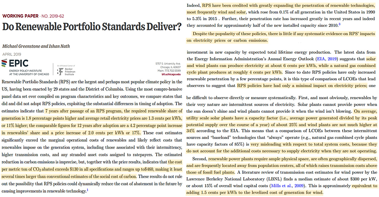
Greenstone and Nath, 2019     RPS [Renewable Portfolio Standards] have been credited with greatly expanding the penetration of renewable technologies, most frequently wind and solar … Despite the popularity of these [Renewable Portfolio Standards] policies, there is little if any systematic evidence on RPS’ impacts on electricity prices or carbon emissions. … The latest data from the Energy Information Administration’s Annual Energy Outlook (EIA, 2019) suggests that solar and wind plants can produce electricity at about 6 cents per kWh, while a natural gas combined cycle plant produces at roughly 4 cents per kWh. … [R]enewables by their very nature are intermittent sources of electricity. Solar plants cannot provide power when the sun doesn’t shine and wind plants cannot provide it when the wind isn’t blowing. On average, utility scale solar plants have a capacity factor (i.e., average power generated divided by its peak potential supply over the course of a year) of about 25% and wind plants are not much higher at 34% according to the EIA. … A literature review of transmission cost estimates for wind power by the Lawrence Berkeley National Laboratory (LBNL) finds a median estimate of about $300 per kW, or about 15% of overall wind capital costs (Mills et al., 2009). This is approximately equivalent to adding 1.5 cents per kWh to the levelized cost of generation for wind. … [E]lectricity prices increase substantially after RPS adoption. The estimates indicate that in the 7th year after passage average retail electricity prices are 1.3 cents per kWh or 11% higher, totaling about $30 billion in the RPS states. And, 12 years later they are 2.0 cents, or 17%, higher. The estimated increases are largest in the residential sector.

Wind Power Harming The Environment, Biosphere

Frondel et al., 2019     Given the rapid expansion of wind power capacities in Germany, this paper estimates the effects of wind turbines on house prices using real estate price data from Germany’s leading online broker. Employing a hedonic price model whose specification is informed by machine learning techniques, our methodological approach provides insights into the sources of heterogeneity in treatment effects. We estimate an average treatment effect (ATE) of up to -7.1% for houses within a one-kilometer radius of a wind turbine, an effect that fades to zero at a distance of 8 to 9 km. …  While the prices of houses close to urban environments are not affected by nearby windmills, houses in rural areas suffer from remarkable devaluation. This effect is even more pronounced for old buildings built prior to 1949, whose asking prices decrease by up to 23%. Our findings can be explained by differences in the appearance of the landscape and preferences of the local population. While the urban population is accustomed to living in an industrialized and dynamic environment, inhabitants of rural areas may lose the impression of pristine nature and tranquility when noise, rotation, and shadow flickers appear. Altogether, our results illustrate that while electricity generation via wind turbines may have global benefits, these are accompanied by substantial local externalities and environmental costs, primarily borne by rural communities close to wind turbines.

Xirouchakis et al., 2019     [T]he environmental impact of commercial wind power production on biodiversity has proved to be substantial [3–7]. Wildlife is affected by wind power production through habitat loss, disturbance and displacement and above all by increased collision risk with wind turbines [8–10]. Bird fatalities due to collision with wind turbines have been the most prominent and frequently identified environmental drawback of wind energy development. Bird casualties from collisions can reach up to 40 deaths per turbine per year [11] with large raptors suffering the greatest toll. … We evaluated the consequences of wind farm development on the griffon vulture (Gyps fulvus) which was regarded as a suitable model species. Griffons are among the most collision-prone large soaring raptors and perhaps the most frequent victims of turbine blades in the Mediterranean region, i.e. up to 1.88 individuals/ turbine/ year [8]. Furthermore, assuming that the most crucial factor in minimizing the negative impact of wind farms on wildlife should be proper siting, we tried to estimate the potential collision mortality of the species by taking into account the existing and all planned wind energy projects on Crete. … Crete holds the last healthy population in the country (ca. 1000 individuals) which constitutes the largest indigenous insular population worldwide. … The model predicted that 39% of the griffon colonies which were occupied by more than 15 individuals would account for 62% of the wind farms and vulture interactions and would suffer 65% of the expected mortalities. The overall collision mortality rate was estimated at 0.03 vultures/wind turbine/year producing an annual loss ranging from 3.7% to 11% of the species population. More specifically a total of 990 individuals were estimated to be at threat of striking with turbine blades. The scenario #1 predicted a mean annual mortality of 1.49 ± 1.12 individuals (range = 0.18–4.98) per colony, whereas the overall annual fatality was anticipated at 83.5 griffons.

Marques et al., 2019     We present evidence that the impacts of wind energy industry on soaring birds are greater than previously acknowledged. In addition to the commonly reported fatalities, the avoidance of turbines by soaring birds causes habitat losses in their movement corridors. … Our findings indicate that the negative effects of wind-power developments on soaring birds may be far more extensive than the commonly reported mortality caused by collision (Marques et al., 2014). Avoidance behaviour may suggest that soaring birds, as well as other birds, are partly able to cope with the existence of wind turbines (Marques et al., 2014). However, our results make clear that this is a simplistic interpretation and may lead to the underestimation of the real impacts of wind-power generation. We recommend that the authorities responsible for wildlife protection and wind industry regulations recognize the loss of aerial habitat caused by wind turbines and the potential associated negative impacts on soaring birds.

Corals Thrive And Grow In Warm, High CO2, And Rising Sea Environments

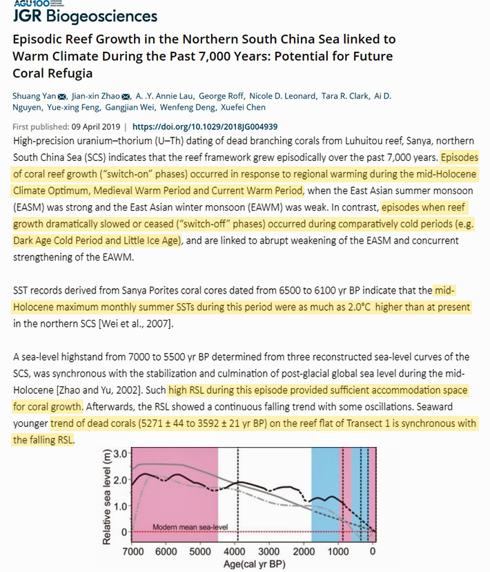
Yan et al., 2019     High-precision uranium–thorium (U–Th) dating of dead branching corals from Luhuitou reef, Sanya, northern South China Sea (SCS) indicates that the reef framework grew episodically over the past 7,000 years. Episodes of coral reef growth (“switch-on” phases) occurred in response to regional warming during the mid-Holocene Climate Optimum, Medieval Warm Period and Current Warm Period, when the East Asian summer monsoon (EASM) was strong and the East Asian winter monsoon (EAWM) was weak. In contrast, episodes when reef growth dramatically slowed or ceased (“switch-off” phases) occurred during comparatively cold periods (e.g. Dark Age Cold Period and Little Ice Age), and are linked to abrupt weakening of the EASM and concurrent strengthening of the EAWM. … SST records derived from Sanya Porites coral cores dated from 6500 to 6100 yr BP indicate that the mid-Holocene maximum monthly summer SSTs during this period were as much as 2.0°C higher than at present in the northern SCS [South China Sea] [Wei et al., 2007]. … A sea-level highstand from 7000 to 5500 yr BP determined from three reconstructed sea-level curves of the SCS, was synchronous with the stabilization and culmination of post-glacial global sea level during the mid-Holocene [Zhao and Yu, 2002]. Such high RSL during this episode provided sufficient accommodation space for coral growth. Afterwards, the RSL showed a continuous falling trend with some oscillations. Seaward younger trend of dead corals (5271 ± 44 to 3592 ± 21 yr BP) on the reef flat of Transect 1 is synchronous with the falling RSL. … All the switch-on episodes are characterized by relatively higher SST and SSS, while the switch-off episodes are associated with lower SST and SSS, concurrent with the centennial to millennial-scale shift of EASM activity. Reconstructions of SST based on Porites from the Leizhou Peninsula [Yu et al., 2005] indicate that while the summer SST maxima were relatively stable (~2°C) over the past 7,000 years, the winter SST minima displayed large variability (up to 5°C) between switch-off and switch-on episodes.

Yokoyama et al., 2019     A sequence of U-series dates obtained from shallowwater corals drilled during Expedition  310 yielded a date for MWP-1A of ~14,600 years ago with a sea level change magnitude of about 16 ± 2 m at a rate of about 40 mm yr–1 (Deschamps et  al., 2012). … In addition, almost 3°–5°C cooling was recorded in the core samples as δ18O and Sr/Ca excursions during the LGM [Last Glacial Maximum] (Felis et al., 2014). These large temperature changes severely impacted the Great Barrier Reef, and together with rapid sea level changes resulted in at least five “near death events” during the last 30,000 years (Webster et al., 2018). The Great Barrier Reef ’s survival of these significant environmental changes may provide a key to understanding the ecological resilience of reef systems (Webster et al., 2018).

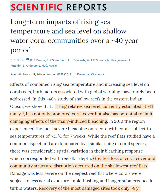
Brown et al., 2019      Effects of combined rising sea temperature and increasing sea level on coral reefs, both factors associated with global warming, have rarely been addressed. In this ~40 y study of shallow reefs in the eastern Indian Ocean, we show that a rising relative sea level, currently estimated at ~11 mm y−1, has not only promoted coral cover but also has potential to limit damaging effects of thermally-induced bleaching. In 2010 the region experienced the most severe bleaching on record with corals subject to sea temperatures of >31 °C for 7 weeks. While the reef flats studied have a common aspect and are dominated by a similar suite of coral species, there was considerable spatial variation in their bleaching response which corresponded with reef-flat depth. Greatest loss of coral cover and community structure disruption occurred on the shallowest reef flats. Damage was less severe on the deepest reef flat where corals were subject to less aerial exposure, rapid flushing and longer submergence in turbid waters. Recovery of the most damaged sites took only ~8 y.

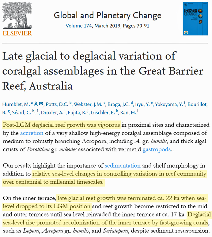
Humblet et al., 2019     Post-LGM [last glacial maximum] deglacial reef growth was vigorous in proximal sites and characterized by the accretion of a very shallow high-energy coralgal assemblage composed of medium to robustly branching Acropora, including A. gr. humilis, and thick algal crusts of Porolithon gr. onkodes associated with vermetid gastropods. … Our results highlight the importance of sedimentation and shelf morphology in addition to relative sea-level changes in controlling variations in reef community over centennial to millennial timescales. … On the inner terrace, late glacial reef growth was terminated at ca. 22 ka when sea-level dropped to its LGM position and reef growth became restricted to the mid and outer terraces until sea level reinvaded the inner terrace at ca. 17 ka. Deglacial sea-level rise promoted recolonization of the inner terrace by fast-growing corals, such as Isopora, Acropora gr. humilis, and Seriatopora, despite sediment resuspension.

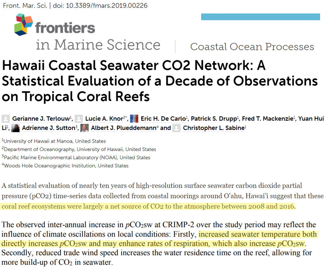
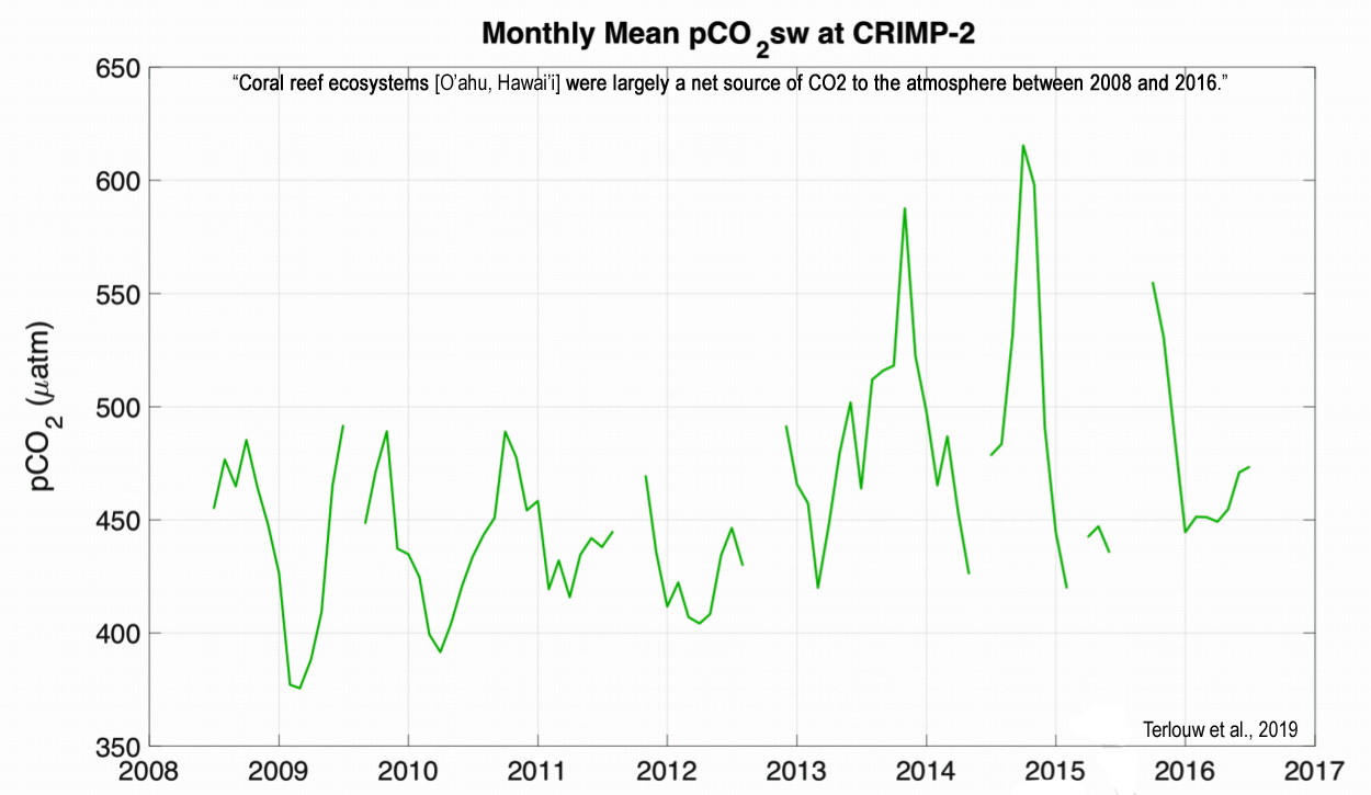
Terlouw et al., 2019A statistical evaluation of nearly ten years of high-resolution surface seawater carbon dioxide partial pressure (pCO2) time-series data collected from coastal moorings around O’ahu, Hawai’i suggest that these coral reef ecosystems were largely a net source of CO2 to the atmosphere between 2008 and 2016. … The observed inter-annual increase in pCO2sw at CRIMP-2 over the study period may reflect the influence of climate oscillations on local conditions: Firstly, increased seawater temperature both directly increases pCO2sw and may enhance rates of respiration, which also increase pCO2sw. Secondly, reduced trade wind speed increases the water residence time on the reef, allowing for more build-up of CO2 in seawater.

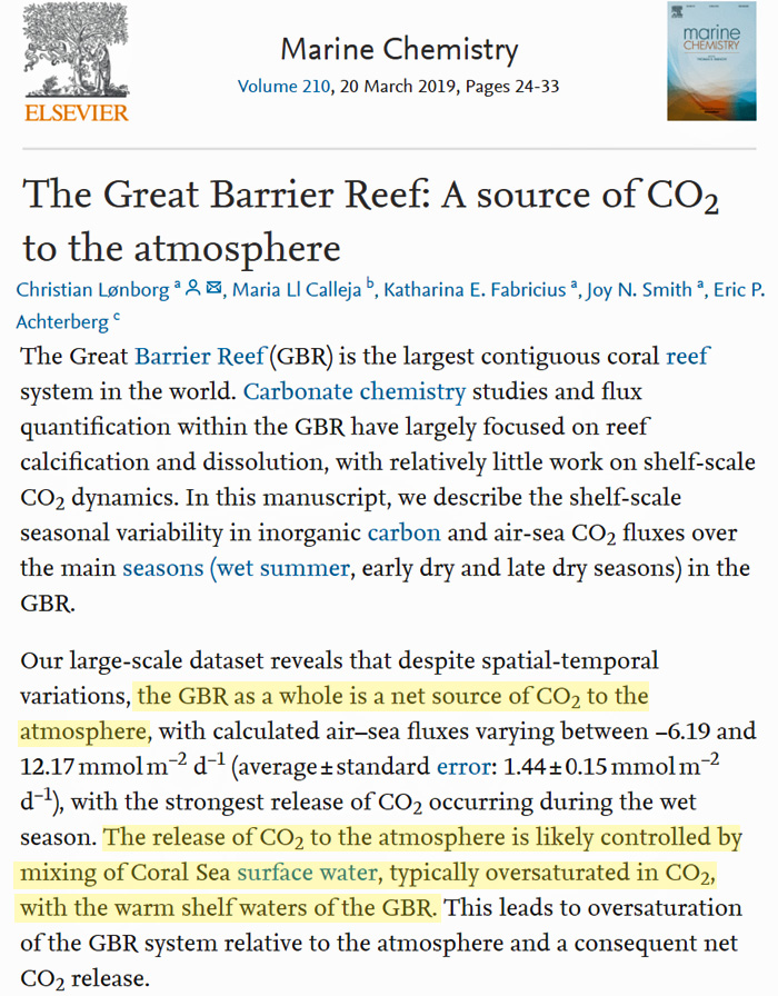
Lønborg et al., 2019     The Great Barrier Reef: A source of CO2 to the atmosphere … Seasonal variations in air-sea CO2 fluxes on the Great Barrier Reef reveal a strong CO2 release during the early-dry season. The Great Barrier Reef is overall a net source of CO2. CO2 fluxes are largely controlled by cross-shelf advection of oversaturated warm surface waters from the Coral Sea.

Elevated CO2, Warmth Does Not Harm The Biosphere

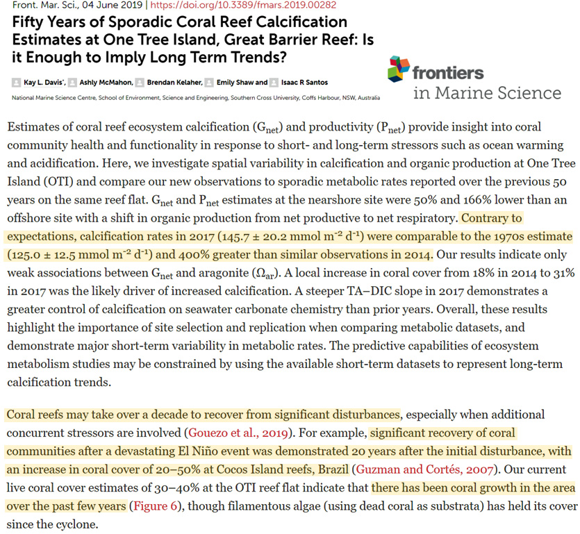
Davis et al., 2019     Estimates of coral reef ecosystem calcification (Gnet) and productivity (Pnet) provide insight into coral community health and functionality in response to short- and long-term stressors such as ocean warming and acidification. Here, we investigate spatial variability in calcification and organic production at One Tree Island (OTI) and compare our new observations to sporadic metabolic rates reported over the previous 50 years on the same reef flat. Gnet and Pnet estimates at the nearshore site were 50% and 166% lower than an offshore site with a shift in organic production from net productive to net respiratory. Contrary to expectations, calcification rates in 2017 (145.7 ± 20.2 mmol m-2 d-1) were comparable to the 1970s estimate (125.0 ± 12.5 mmol m-2 d-1) and 400% greater than similar observations in 2014. … Coral reefs may take over a decade to recover from significant disturbances, especially when additional concurrent stressors are involved (Gouezo et al., 2019). For example, significant recovery of coral communities after a devastating El Niño event was demonstrated 20 years after the initial disturbance, with an increase in coral cover of 20–50% at Cocos Island reefs, Brazil (Guzman and Cortés, 2007). Our current live coral cover estimates of 30–40% at the OTI reef flat indicate that there has been coral growth in the area over the past few years, though filamentous algae (using dead coral as substrata) has held its cover since the cyclone.

Kersting and Linares, 2019     These findings provide a link between rejuvenescence in fossil and extant corals and reveal that beyond adaptation and acclimatization processes, modern scleractinian corals show yet undiscovered and highly effective survival strategies that help them withstand and recover from rapid environmental changes.

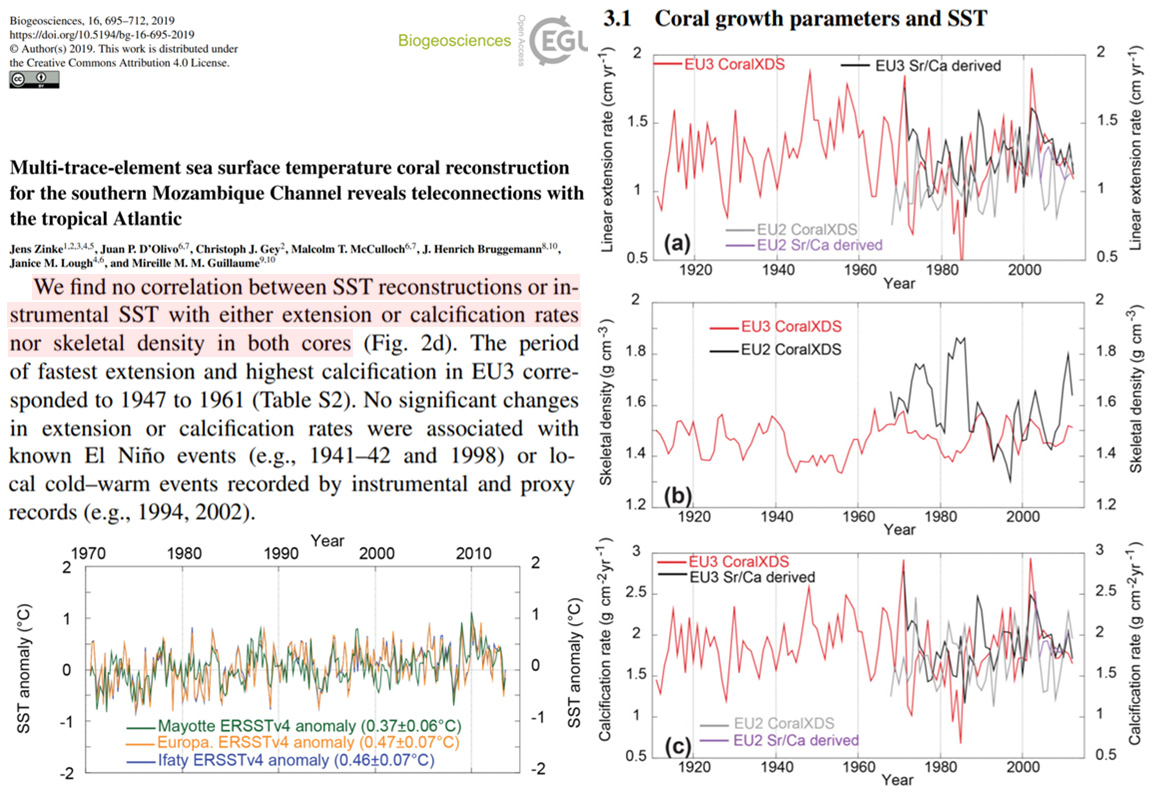
Zinke et al., 2019     We find no correlation between SST reconstructions or instrumental SST with either extension or calcification rates nor skeletal density in both cores (Fig. 2d). The period of fastest extension and highest calcification in EU3 corresponded to 1947 to 1961 (Table S2). No significant changes in extension or calcification rates were associated withknown El Niño events (e.g., 1941–42 and 1998) or local cold–warm events recorded by instrumental and proxy records (e.g., 1994, 2002).

Gouezo et al., 2019     Our study documents that the time needed for coral reefs to recover from bleaching disturbance to coral-dominated state in disturbance-free regimes is at least 9–12 years. Importantly, we show that reefs in two habitats achieve relative stability to a climax community state within that time frame.

Vasconcelos et al., 2019     Coral reef growth pattern in eastern Brazil has not changed since the Holocene …  The coral fauna that built the reefs did not change much since the beginning of reef growth (approximately 7,000 yr BP), suggesting that the environmental conditions in this region have most likely remained favorable for the development of coral reefs. The coral fauna that built the Brazilian reefs is mostly composed of resistant and well-adapted endemic coral species, which biodiversity has remained constant throughout the development of the reefs.

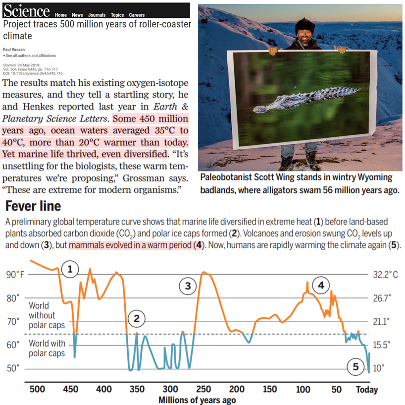
Voosen, 2019     Some 450 million years ago, ocean waters averaged 35°C to 40°C, more than 20°C warmer than today. Yet marine life thrived, even diversified.

Balasooriya et al., 2019     Elevated [CO2 ] and higher temperature caused significant increases in total polyphenol, flavonoid, anthocyanin and antioxidants in both strawberry cultivars when compared with plants grown under ambient conditions. Results of HPLC-UV analysis also revealed that individual phenolic compounds of fruits were also increased with increasing [CO2 ] and temperature. … Strawberry fruit was rich with polyphenols and antioxidants when grown under elevated [CO2 ] and higher temperature. There were also interactions between [CO2 ] and temperature affecting the fruits’ content. An increase in the polyphenol and antioxidant content in strawberry fruits would be highly beneficial to human health.

Munday et al., 2019     Specifically, we reared kingfish to 21 days post hatching (dph) in a fully crossed 2 × 2 experimental design comprising current-day average summer temperature (21°C) and seawater pCO2 (500 μatm CO2) and elevated temperature (25°C) and seawater pCO2 (1,000 μatm CO2). … Elevated temperature, but not elevated CO2 affected all morphological traits. Weight, length and other morphological traits in juvenile yellowtail kingfish exhibited low but significant heritability under current day and elevated temperature. However, there were no measurable GxE interactions in morphological traits between the two temperature treatments at 21 dph. Similarly, there was no detectable change in any of the measures of genetic diversity over the duration of the experiment. Nonetheless, one family exhibited differential survivorship between temperatures, declining in relative abundance between 1 and 21 dph at 21°C, but increasing in relative abundance between 1 and 21 dph at 25°C. This suggests that this family line could perform better under future warming than in current-day conditions. Our results provide the first preliminary evidence of the adaptive potential of a large pelagic fisheries species to future ocean conditions.

No Effect Of Elevated CO2 (5000-15,000 ppm) On Human Cognition, Health

Monsé et al., 2019     Potash miners can become exposed to carbon dioxide (CO2) during the blasting of basalt intrusions or loading and transporting the blasted salt. In a cross-shift study, we compared physiological effects of acute exposure to elevated CO2 concentrations in miners after long-term exposure to evaluate the possible health risks. A group of 119 miners was assessed by clinical examination, lung function tests, and blood gas content directly before and after the shift. A cumulative CO2 exposure was measured using personal monitors. The miners were categorized as low (<0.1 vol.% [less than 1,000 ppm], n = 83), medium (<0.5 vol.% [1,000 to 5,000 ppm], n = 26), and high (>0.5 vol.% [5,000 to 15,000 ppm], n = 10) CO2 exposed subjects. We found no significant differences among the three groups. Lung function testing revealed no conspicuous findings, and chronic health effects were not observed in the miners either. In conclusion, no significant adverse effects could be found in potash miners exposed to elevated CO2 concentrations. Therefore, the mining authorities allow potash mining operations for 4 h at ambient CO2 up to 1.0 vol.% and for 2 h at CO2 not exceeding 1.5 vol.% per shift.

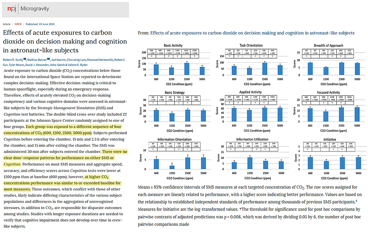
Scully et al., 2019      Effects of acutely elevated CO2 on decision-making competency and various cognitive domains were assessed in astronaut-like subjects by the Strategic Management Simulation (SMS) and Cognition test batteries. The double-blind cross-over study included 22 participants at the Johnson Space Center randomly assigned to one of four groups. Each group was exposed to a different sequence of four concentrations of CO2 (600, 1200, 2500, 5000 ppm). Subjects performed Cognition before entering the chamber, 15 min and 2.5 h after entering the chamber, and 15 min after exiting the chamber. The SMS was administered 30 min after subjects entered the chamber. There were no clear dose–response patterns for performance on either SMS or Cognition. Performance on most SMS measures and aggregate speed, accuracy, and efficiency scores across Cognition tests were lower at 1200 ppm than at baseline (600 ppm); however, at higher CO2 concentrations performance was similar to or exceeded baseline for most measures. These outcomes, which conflict with those of other studies, likely indicate differing characteristics of the various subject populations and differences in the aggregation of unrecognized stressors, in addition to CO2, are responsible for disparate outcomes among studies. Studies with longer exposure durations are needed to verify that cognitive impairment does not develop over time in crew-like subjects.

Elevated CO2: Greens Planet, Higher Crop Yields

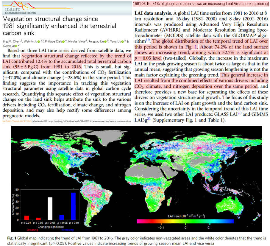
Chen et al., 2019     The global distribution of the temporal trend of LAI [leaf area index, greening] over this period [1981-2016] is shown in Fig. 1. About 74.2% of the land surface shows an increasing trend, among which 52.7% is significant at p = 0.05 level (two-tailed). Globally, the increase in the maximum LAI in the peak growing season is about twice as large as that in the annual mean, suggesting that growing season lengthening is not the main factor explaining the greening trend. This general increase in LAI resulted from the combined effects of various drivers including CO2, climate, and nitrogen deposition over the same period, and therefore provides a new base for separating the effects of these drivers on vegetation structure and growth. … Based on three LAI time series derived from satellite data, we find that vegetation structural change reflected by the trend of LAI [leaf area index/greening] contributed 12.4% to the accumulated total terrestrial carbon sink (95 ± 5 Pg C) from 1981 to 2016. This is small, but significant, compared with the contributions of CO2 fertilization (+47.0%) and climate change (−28.6%) in the same period. This finding suggests the importance in tracking this vegetation structural parameter using satellite data in global carbon cycle research. Quantifying this separate effect of vegetation structural change on the land sink helps attribute the sink to the various drivers including CO2 fertilization, climate change, and nitrogen deposition, and may also help rectify some differences among prognostic models.

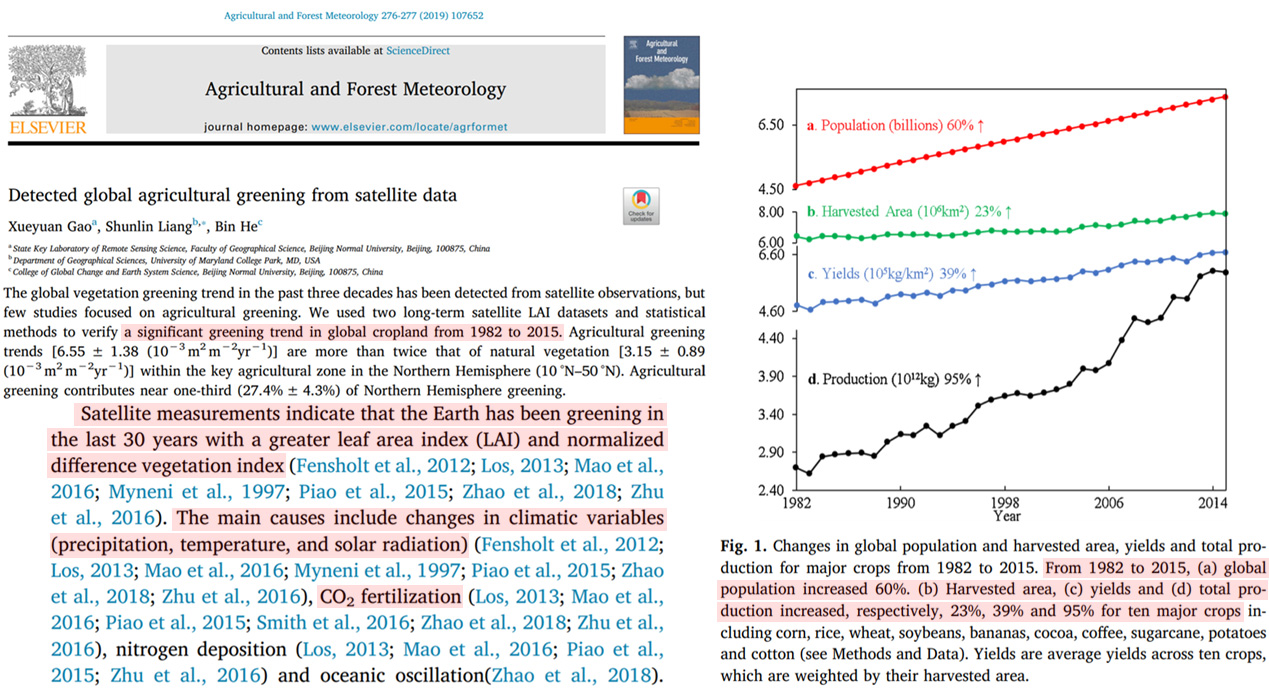
Gao et al., 2019     The global vegetation greening trend in the past three decades has been detected from satellite observations, but few studies focused on agricultural greening. We used two long-term satellite LAI datasets and statistical methods to verify a significant greening trend in global cropland from 1982 to 2015. Agricultural greening trends [6.55 ± 1.38 (10−3 m2 m−2yr−1)] are more than twice that of natural vegetation [3.15 ± 0.89 (10−3 m2 m−2yr−1)] within the key agricultural zone in the Northern Hemisphere (10 °N–50 °N). Agricultural greening contributes near one-third (27.4% ± 4.3%) of Northern Hemisphere greening. …  From 1982 to 2015, (a) global population increased 60%. (b) Harvested area, (c) yields and (d) total production increased, respectively, 23%, 39% and 95% for ten major crops including corn, rice, wheat, soybeans, bananas, cocoa, coffee, sugarcane, potatoes and cotton.

Oliveira and Malenco, 2019     Climate models predict an increase in atmospheric CO2 concentration and prolonged droughts in some parts of the Amazon, but the effect of elevated CO2 is still unknown. Two experiments (ambient CO2 ‒ 400 ppm and elevated CO2 ‒ 700 ppm) were conducted to assess the effect of drought (soil at 50% field capacity) on physiological parameters of Carapa. At ambient CO2 concentration, light-saturated net photosynthetic rate (PNsat) was reduced by 33.5% and stomatal conductance (gs) by 46.4% under drought, but the effect of drought on PNsat and gs was nullified at elevated CO2. Total plant biomass and leaf area production were also reduced (42‒47%) by drought. By changing leaf traits, Carapa is able to endure drought, as the consumptive use of water was reduced under drought (32‒40%). The improvement of PNsat under elevated CO2 and water stress and the leaf plasticity of Carapa broaden our understanding of the physiology of Amazonian trees.

Chen et al., 2019     Satellite data show increasing leaf area of vegetation due to direct factors (human land-use management) and indirect factors (such as climate change, CO2 fertilization, nitrogen deposition and recovery from natural disturbances). Among these, climate change and CO2 fertilization effects seem to be the dominant drivers. However, recent satellite data (2000–2017) reveal a greening pattern that is strikingly prominent in China and India and overlaps with croplands world-wide. China alone accounts for 25% of the global net increase in leaf area with only 6.6% of global vegetated area. The greening in China is from forests (42%) and croplands (32%), but in India is mostly from croplands (82%) with minor contribution from forests (4.4%).

Jacotot et al., 2019     Our results showed that elevated CO2 [800 ppm]  increased the growth rates of both A. marina and R. stylosa, for which the final biomass was, respectively, 46 and 32% higher than in the ambient CO2 treatment [400 ppm]. We suggest that this increase was driven by a stimulation of photosynthesis under elevated CO2, as demonstrated in a previous study.

He  et al., 2019     The results show that above three indicators all point to a little change in aridity of drylands over the past three decades, and their trends in spatial patterns agree well each other. Simultaneously, significant greening (p < 0.05) occurred in more than 36% of vegetated drylands, in contrast to the 7% with significant browning (p < 0.05). Drylands as a whole, vegetative greenness demonstrated a significant positive relationship (p < 0.05) with precipitation change. At the biome scale, significant relationships (p < 0.05) were observed for vegetative greenness and precipitation for all other vegetation types except forests, suggesting that the increasing precipitation was one of the main drivers of greening over drylands.

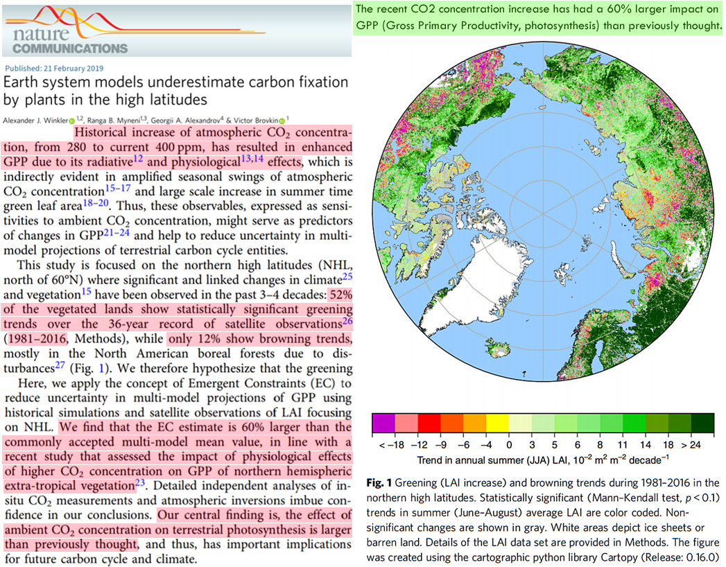
Winkler et al., 2019     Historical increase of atmospheric CO2 concentration, from 280 to current 400 ppm, has resulted in enhanced GPP [gross primary production/greening] due to its radiative and physiological effects, which is indirectly evident in amplified seasonal swings of atmospheric CO2 concentration and large scale increase in summer time green leaf area. Thus, these observables, expressed as sensitivities to ambient CO2 concentration, might serve as predictors of changes in GPP and help to reduce uncertainty in multimodel projections of terrestrial carbon cycle entities. This study is focused on the northern high latitudes (NHL, north of 60°N) where significant and linked changes in climate and vegetation have been observed in the past 3–4 decades: 52% of the vegetated lands show statistically significant greening trends over the 36-year record of satellite observations (1981–2016, Methods), while only 12% show browning trends, mostly in the North American boreal forests due to disturbances. … Here, we apply the concept of Emergent Constraints (EC) to reduce uncertainty in multi-model projections of GPP using historical simulations and satellite observations of LAI focusing on NHL. We find that the EC estimate [of the effect of CO2 on greening/GPP] is 60% larger than the commonly accepted multi-model mean value, in line with a recent study that assessed the impact of physiological effects of higher CO2 concentration on GPP of northern hemispheric extra-tropical vegetation. Detailed independent analyses of insitu CO2 measurements and atmospheric inversions imbue confidence in our conclusions. Our central finding is, the effect of ambient CO2 concentration on terrestrial photosynthesis is larger than previously thought, and thus, has important implications for future carbon cycle and climate.

Qiao et al., 2019     Maize had 25% yield increase under elevated temperature (eT). Soybean had 31% yield increase under elevated CO2 (eCO2) with eT. Elevated temperature with and without eCO2 increased grain oil concentrations.

Brandt et al., 2019     Recent Earth observation studies find a greening of the Earth and in particular in global drylands, which is commonly interpreted as a global increase in net primary production and has been attributed to climate change. Although changes in rainfall, fire regimes, elevated temperatures, atmospheric CO2 and nitrogen depositions are suggested explanations, only few studies provide quantitative evidence on both the biophysical processes (changes in vegetation cover, structure and composition) and controlling factors of long-term dryland vegetation trends.

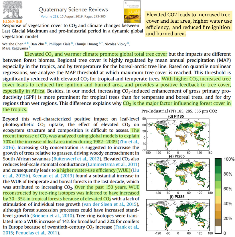
Cernusak et al., 2019     Human-caused CO2 emissions over the past century have caused the climate of the Earth to warm and have directly impacted on the functioning of terrestrial plants. We examine the global response of terrestrial gross primary production (GPP) to the historic change in atmospheric CO2. The GPP of the terrestrial biosphere has increased steadily, keeping pace remarkably in proportion to the rise in atmospheric CO2. Water-use efficiency, namely the ratio of CO2 uptake by photosynthesis to water loss by transpiration, has increased as a direct leaf-level effect of rising CO2. This has allowed an increase in global leaf area, which has conspired with stimulation of photosynthesis per unit leaf area to produce a maximal response of the terrestrial biosphere to rising atmospheric CO2 and contemporary climate change.

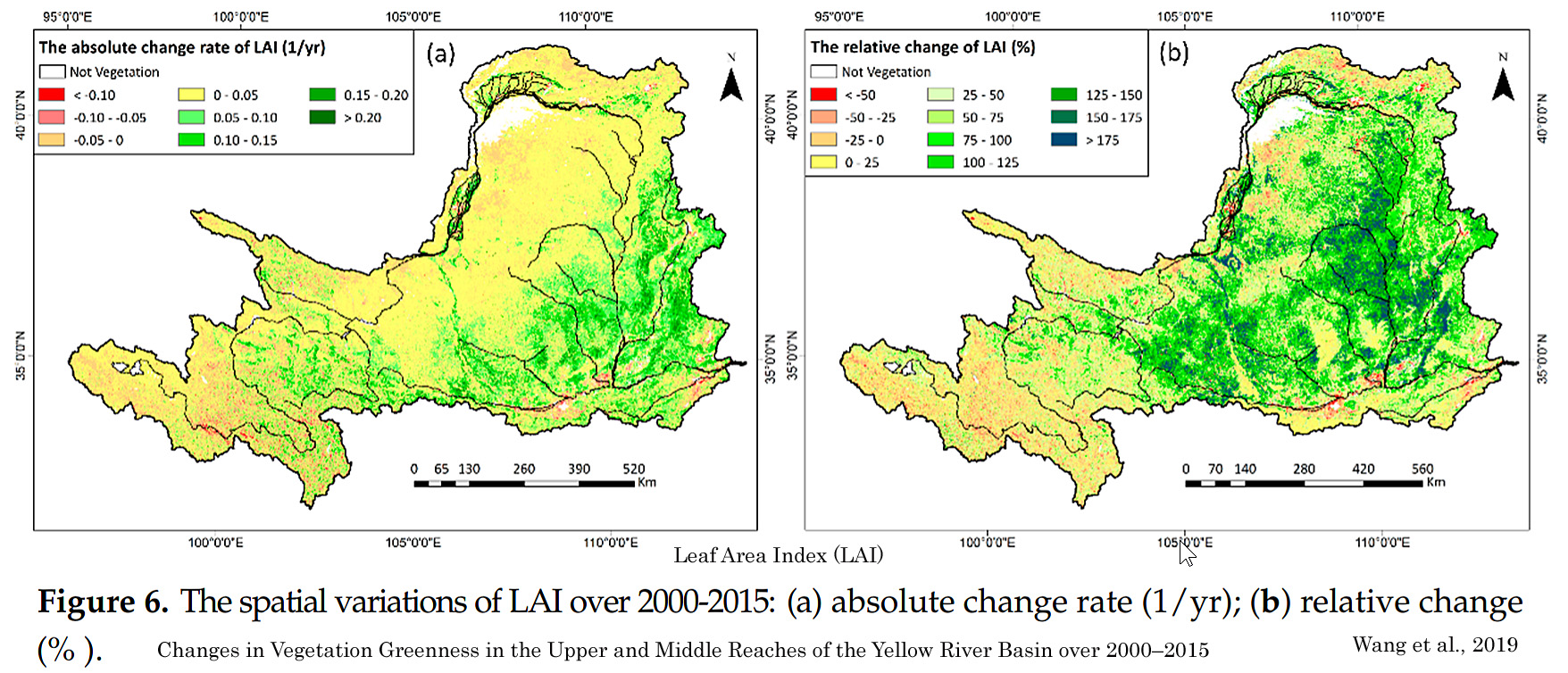
Wang et al., 2019     Changes in Vegetation Greenness in the Upper and Middle Reaches of the Yellow River Basin over 2000–2015 … In this study, the vegetation dynamic characteristics were analyzed for unconverted forestland, shrubland, grassland, cropland, and converted forestland, shrubland, and grassland from cropland over 2000–2015 in the upper and middle reaches of the Yellow River. … The results obtained were as follows: (1) Vegetation greening was remarkable in the entire study region (0.036 yr−1). … Overall greening trend in the upper and middle reaches of the Yellow River indicated great achievements have been obtained since the implementation of the GTGP. Vegetation restoration exerted stronger influences on converted types from cropland than unconverted types. In the future, approximately 73.1% of the study region is expected to continue increasing [greening].

Zhang et al., 201      While summer GST [ground surface temperature] had a somewhat consistently positive correlation with tree growth, winter GST has shifted from a negative to a strongly positive correlation with growth in the last decade, coincidental with a sharp increase in winter GST since 2004. Winter GST is also strongly correlated with the rapidly thawing permafrost dynamics. Overall, our results suggest a link between recent changes in the permafrost and shifts in climate‐growth correlations for one of the main boreal tree species. As a result, L. gmelinii has experienced an important increase in radial growth that may indicate that, unlike what has been reported for other boreal species, it may temporally benefit from warming climate in the continuous permafrost region of the Asian boreal forests.

Oliveira and Marenco, 2019     The large increase in total biomass and the substantial improvement in WUEP [water use efficiency] under eCO2 [elevated CO2, 700 ppm], and the sharp decline in leaf area under water stress widen our knowledge on the physiology of this important species for the forest management of large areas in the Amazon region.

Gulyás et al., 2019     Due to climate change, it is important to know to what extent forests will be impacted by atmospheric changes. This study focuses on the height growth response of sessile oak … The relative top heights of the young stands were significantly higher than of the older stands, which means that the overall growing conditions were better in the last 30-35 years due to atmospheric changes than the mean conditions during the lifetime of old stands.

Chen et al., 2019     With higher CO2, increased tree cover leads to reduced fire ignition and burned area, and provides a positive feedback to tree cover, especially in Africa. Besides, in our model, increasing CO2-induced enhancement of gross primary productivity (GPP) is more prominent for tropical trees than for temperate and boreal trees, and for dry regions than wet regions. This difference explains why CO2 is the major factor influencing forest cover in the tropics.

Qiu et al., 2019    Our results show that both net primary production (NPP) and heterotrophic respiration (HR) of northern peatlands increased over the past century in response to CO2 and climate change.

Yu et al., 2019    Vegetation shows a greening trend on the global scale in the past decades, which has an important effect on the hydrological cycle, and thus quantitative interpretation of the causes for vegetation change is of great benefit to understanding changes in ecology, climate, and hydrology. … The estimated change trend in leaf area index (LAI) is 1.20%/year from 2001 to 2017, which accounts for approximately half of the observed (2.31%/year) by the moderate resolution imaging spectroradiometer (MODIS). Regarding the causes for vegetation greening, the contributions of: (1) LULCC [land use and land cover change]; (2) atmospheric CO2 concentration; and (3) vapor pressure deficit were: (1) 88.3%; (2) 40.0%; and (3) −28.3%, respectively, which reveals that the largest contribution was from LULCC, which is probably driven by increased total water availability in whole oasis with a constant transpiration in vegetation area. The improved Donohue13 model, a simple but physics-based model, can partially explain the impact of factors related to climatechange and anthropogenic activity on vegetation change in arid regions. It can be further combined with the Budyko hypothesis to establish a framework for quantifying the changes in coupled response of vegetation and hydrological processes to environment changes.

Sakai et al., 2019     We conducted free-air CO2 enrichment (FACE) experiments in 2 years to examine whether rice cultivars bred in different eras differ in response to E-[CO2] [elevated CO2] and to determine any associated traits. We tested five Japanese cultivars: Aikoku (released in 1882), Norin 8 (1934), Koshihikari (1956), Akihikari (1976) and Akidawara (2009). The yields of Aikoku and Norin 8 increased by 19.3% and 30.3%, respectively, under E-[CO2], while those of Koshihikari and Akihikari increased by 15.9% and 3.4%, respectively. However, that of Akidawara, the newest cultivar, also increased by 19.0%.

Hazra et al., 2019     Elevated CO2 (+50% higher than ambient) increased wheat grain yield by 17% in subtropical Eastern India.

Pastore et al., 2019     Here, we report the effects of eCO2 [elevated CO2] on rates of net photosynthesis and stomatal conductance in 14 perennial grassland species from four functional groups over two decades in a Minnesota Free‐Air CO2 Enrichment experiment, BioCON. … Leaf‐level water‐use efficiency increased by 50% under eCO2 [elevated CO2] primarily because of reduced stomatal conductance. Our results imply that enhanced nitrogen supply will not necessarily diminish photosynthetic acclimation to eCO2 in nitrogen‐limited systems, and that significant and consistent declines in stomatal conductance and increases in water‐use efficiency under eCO2 [elevated CO2] may allow plants to better withstand drought.

Niu et al., 2019     The ratio of transpiration to total terrestrial evapotranspiration (T/ET) plays an important role in the hydrological cycle and in the energy budgets between the land and the atmosphere. Although China has experienced substantial climate warming and vegetation restoration (i.e., greening) over the past decades, the response of T/ET to the changing climate and environmental factors is poorly understood. Here, we apply a model-data fusion method that integrates the Priestly-Taylor Jet Propulsion Laboratory (PT-JPL) model with multivariate observational datasets (transpiration and evapotranspiration) to quantify the relative contributions of multiple factors to the T/ET trend for the terrestrial ecosystem of China from 1982 to 2015. Validation against the observational data indicates that the PT-JPL model performed well. The multi-year average T/ET was estimated to be 0.56 ± 0.05 in China. The T/ET of the forest ecosystems (0.65–0.72) was generally higher than that of the non-forest ecosystems (0.41–0.60). T/ET increased remarkably at a rate of 0.0019 yr−1 (P < 0.01) during the study period. Leaf area index increased significantly over the period, by 0.0031 m2 m−2 yr−1. It appears that greening and climate change were the most likely causes of the increasing T/ET in China, directly explaining 57.89% and 36.84% of the T/ET trend, respectively. Particularly, in the subtropical-tropical monsoonal region, greening directly contributed 24.43% to the T/ET trend whereas climate change contributed 60.95%. The influences of greening and climate change on T/ET trends are mutually reinforcing.

Raj et al., 2019     Climate  change  associated  with  rising  atmospheric  carbon  dioxide  (CO2)  concentration  may  have  impact  on  crop production and soil health. Increase in atmospheric CO2 concentration may enhance crop growth with higher demand for nutrients by the crop. An experiment was conducted during July-October, 2013 using Free Air Carbon Dioxide Enrichment facility at the Indian Agricultural Research Institute, New Delhi to study the impact of elevated CO2 and nitrogen (N) dose on growth, yield and nitrogen uptake in rice crop. Four doses of N, i.e., control, 0.6 g N pot-1 (75% recommended dose of N), 0.8 g N pot-1 (100% recommended dose of N) and 1.0 g N pot-1 (125% recommended dose of N) were applied in both ambient (395 ppm) and elevated CO2 (550±20 ppm)  conditions. Grain and biomass yield of rice was significantly higher under elevated CO2 condition. Plant growth and yield parameters also increased with increased N doses in both elevated and ambient CO2 conditions. Nitrogen concentration of grain and straw decreased under high CO2 level but N uptake increased under elevated CO2 condition. Agronomic efficiency of N was higher under elevated CO2 while recovery efficiency of N remained unaffected. The study showed that although yield of rice increases under elevated CO2 condition, to maintain plant nitrogen concentration, application of additional dose of N is required.

O’Sullivan et al., 2019     The recent warming hiatus (1998–2013) was identified as a potential key mechanism behind the increased land sink during this period via reduced ecosystem respiration (Ballantyne et al., 2017). … At the global scale, simulated NPP [net primary production, greening] increased substantially over the 20th century to present day from 56.2 (mean of 1901–1910) to 66.0 Pg C/year (mean of 2007–2016) with positive contributions from all drivers considered, including rising CO2 concentrations (referred to as CO2 fertilization), nitrogen deposition, climate, and carbon‐nitrogen as well as carbon‐climate synergies. The relative contribution of these drivers to this overall NPP increase amounts to 60% for increased CO2, 15% for nitrogen deposition, 8% for carbon‐nitrogen synergy, 9% for carbon‐climate synergy, and 8% for climate. Both CO2 fertilization and nitrogen deposition individually caused a smooth, transient increase in NPP, in line with the trajectory of the corresponding drivers …  [R]esults show a global NPP [net primary production, greening] increase of 3.4 Pg C/year between the early 1990s (mean of 1990–1996) and the end of our study period (2010–2016), with CO2 fertilization and climate being the dominant drivers, accounting for 56% and 35% of the overall change, respectively. … Carbon‐climate interactions led to significant increases in tropical forests and the forests of North America, Eurasia, and China.

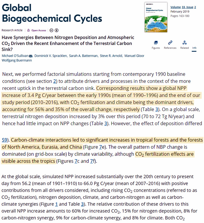
Lu et al., 2019     The strong response of terrestrial carbon pool to the change of pCO2 is further investigated in a series of pCO2 sensitivity experiments. The biosphere total carbon stock is increased by elevated pCO2, but the CO2 fertilization effect tends to saturate at higher pCO2 due to soil nitrogen availability (Smith et al. 2014; Wårlind et al. 2014). …  pCO2 as a single factor explains about 70% and 80% of the increased NPP and land carbon pool, respectively (Fig. 2 d1, red; 3b, red ‘−CO2’). A secondary contribution to enhanced NPP comes from vegetation expansion forced by higher temperatures, but only from glacial cold temperature to PI at high latitudes. … The carbon flux and carbon storage variations of the terrestrial biosphere under past cold and warm climate episodes can be partitioned among the effects of the four forcing factors. The most striking feature is that these variations are primarily controlled by pCO2 (Schimel et al. 2015).

Bencke-Malato et al., 2019     In this study, we evaluated the individual and combinatory effects of E[CO2] [elevated CO2] and water deficit on the physiology and root molecular responses in soybean. Plants growing under E[CO2] [elevated CO2] exhibited increased photosynthesis that resulted in a higher biomass, plant height, and leaf area. E[CO2] decreased the transcripts levels of genes involved in iron uptake and transport, antioxidant activity, secondary metabolism and defense, and stress responses in roots. When plants grown under E[CO2] [elevated CO2] are treated  with instantaneous water deficit, E[CO2] reverted the expression of water deficit-induced genes related to stress, defense, transport and nutrient deficiency. Furthermore, the interaction of both treatments uniquely affected the expression of genes. Both physiological and transcriptomic analyses demonstrated that E[CO2] may mitigate the negative effects of water deficit on the soybean roots.

Parvin et al., 2019     Free air CO2 enrichment (FACE) improves water use efficiency and moderates drought effect on N2 fixation of Pisum sativum L. … This study suggests that e[CO2] [elevated CO2] increased WUE [water use efficiency] and this resulted in slower soil water depletion, allowing pea plants to maintain greater nodule activity under drought and resulting in appreciable increases in N2 fixation. Our results suggest that growth under e[CO2] can mitigate drought effects on N2 fixation and reduce dependency on soil N resources especially in water-limited agro-ecosystems.

Li et al., 2019     Drought induced a significant increase in leaf and spike abscisic acid concentrations, while elevated [CO2] showed no effect. At maturity, post‐anthesis drought and heat stress significantly decreased the grain yield by 21.3%–65.2%, while elevated [CO2] increased the grain yield by 20.8% in wheat, which was due to the changes of grain number per spike and thousand grain weight. This study suggested that the responses of plant water status and grain yield to extreme climatic events (heat and drought) can be influenced by the atmospheric CO2 concentration.

Fire Frequency Stable or Declining

Abrams and Nowacki, 2019     Modern assemblages comprise tree genera that are increasingly cool-adapted, shade-tolerant, drought-intolerant pyrophobes. Paleocharcoal data from 1 to 1750 AD indicate a slight increase in burning in southern forests and stable levels in the north, despite the increasing cold associated with the Little Ice Age. … After 1750 AD, charcoal levels in the southern zone form a parabola, increasing rapidly, cresting around 1900, then declining thereafter. … A decline in recent centuries is also evident in the south and the eastern USA as a whole. … The most noticeable feature of the 2000-year fire history here is a large increase in burning during the past ~300 years associated with European land clearance for agriculture. Biomass burning peaked between 1800 and 1900 AD based on historical records, followed by substantial declines after ca. 1940. … The charcoal index between 1 and 1750 AD in this study suggests stable levels of burning in the north and a slight increase in the south. It is interesting to note that southern forests exhibited a slight increase in burning associated with the Medieval Warm Period (ca. 950 to 1250 AD) but did not decline with the LIA (ca. 1350–1850; Mann et al. 2009). In northern forests, the charcoal index dipped between 1000 and 1200 AD and then increased at the start of the LIA, the opposite of what would be expected from climate control. … The large decrease in fire after 1940, mainly attributed to active fire suppression via the Smokey Bear campaign (Abrams 2010), occurred during a significant warming period and may represent another important fire-climate disconnect. However, the decline of burning may have been facilitated by lessening frequency and intensity of drought after 1930 (Fig. 1; McEwan et al. 2011).

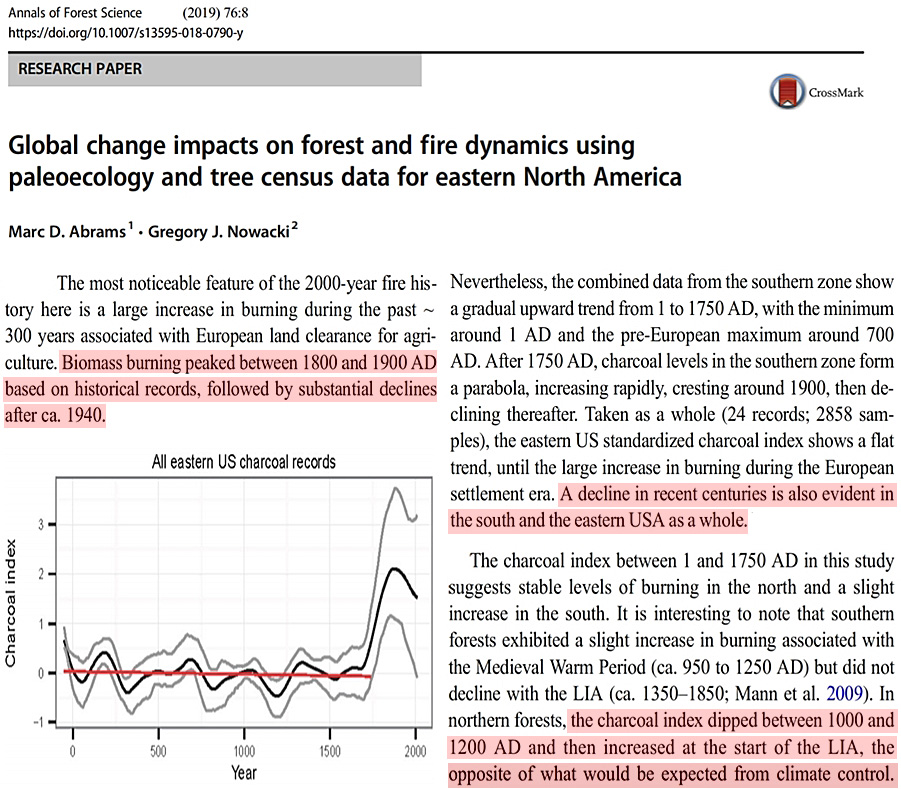
Bobek et al., 2019     Our results suggest that rising vegetation productivity driven by rapid Early Holocene climate amelioration enhanced biomass burning. The increased fire activity during this period was driven by both a drier- and warmer-than-present climate and easily flammable fuels produced by conifer-dominated vegetation. We identified an inhibiting effect of the concomitant Fagus sylvatica expansion on levels of biomass burning that occurred asynchronously between our mountain and mid-elevation sandstone regions 6500 cal yr BP and 4900 cal yr BP, respectively. The amount of compositional change in plant communities was more related to the transformation of major vegetation types than to fluctuations in fire activity levels. The divergent timing of the fire decline in response to the Fagus sylvatica expansion implies biotic control over biomass burning that is independent of a direct climatic influence.

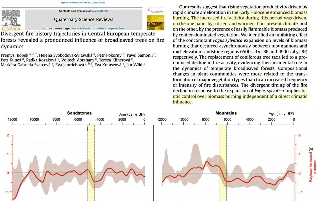
Mass and Ovens, 2019     The lack of correlation between late summer/autumn wildfires over central coastal California and summer precipitation or temperature weakens the potential connection of the current coastal California wildfires with anthropogenic global warming. … Most of the largest coastal California wildfire events have been associated with strong offshore winds: Santa Ana and sundowner winds over Southern California, and Diablo winds over the central and northern coastal areas of the state. There is no reason to expect that strong offshore winds in autumn have increased or will increase due to anthropogenic global warming; in fact, the opposite may be the case, since model projections suggest that anthropogenic global warming will warm the interior more than the coastal zone, preferentially reducing pressure over the inland region, thus reducing the offshore pressure gradient (e.g., Hughes et al. 2009). As described earlier in the paper, one weather/climate variable that does correlate with fall wildfire frequency and area burned over coastal California, above-normal precipitation during the previous winter, does not appear to have been enhanced by the anthropogenic global warming of the past decades. As shown in Fig. 6, there has been no observed trend during the past half-century in extreme winter precipitation over coastal California. Furthermore, studies using climate model simulations driven by increasing greenhouse gas concentrations (e.g., Swain et al. 2018) do not suggest an increase in heavy precipitation events during the contemporary period. … Finally, there is no long-term trend in the number of wildfires over coastal California (Dennison et al. 2014), a trend that might be consistent with a small role of anthropogenic climate change driven by increasing greenhouse gases, or the result of compensation between a number of competing factors.

 

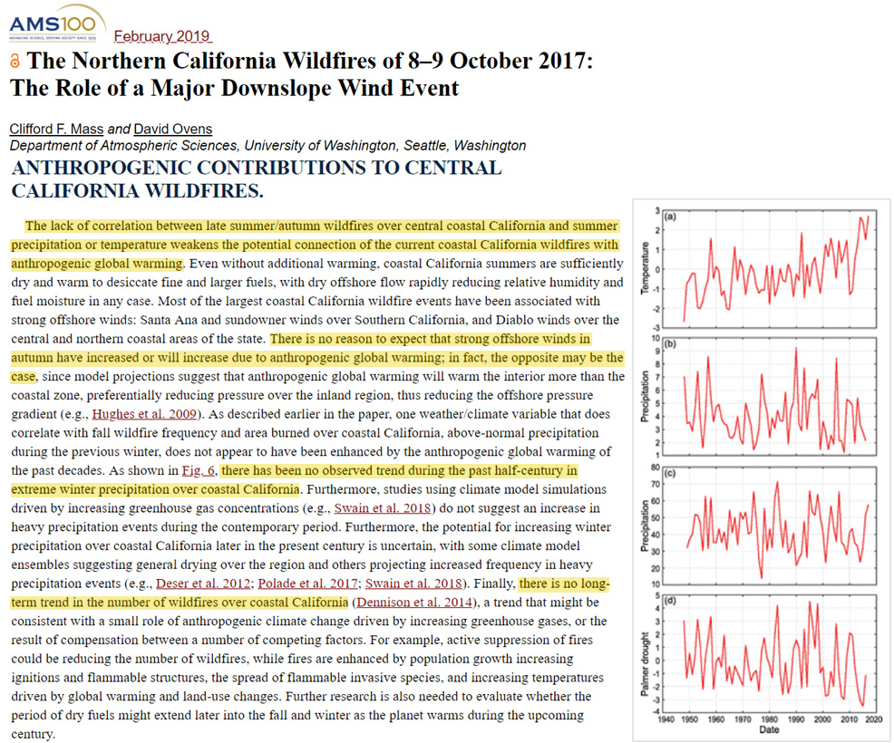
Global Warming Reduces Mortality. Cold Kills.

Cheng et al., 2018     We collected daily time-series data on all-cause deaths and weather variables for the five most populous Australian cities (Sydney, Melbourne, Brisbane, Adelaide, and Perth), from 2000 to 2009. … The greatest percentage increase in mortality was for cold (2.0%, 95% confidence interval (CI): 1.4%, 2.6%), followed by heat (1.2%, 95% CI: 0.7%, 1.7%), and temperature variability (0.5%, 95% CI: 0.3%, 0.7%). There was no clear temporal pattern in mortality risk associated with any temperature exposure in Australia. Heat, cold and temperature variability together resulted in 42,414 deaths during the study period, accounting for about 6.0% of all deaths. Most of attributable deaths were due to cold (61.4%), and noticeably, contribution from temperature variability (28.0%) was greater than that from heat (10.6%).

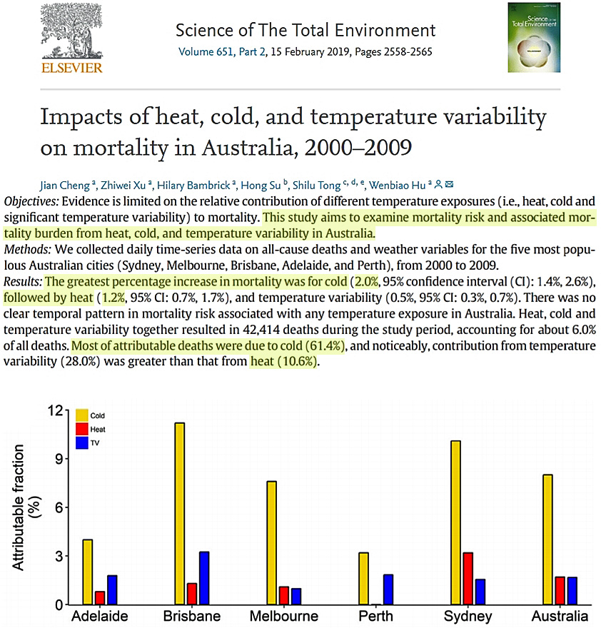
Deng et al., 2019     Using daily mortality and meteorological data from 2009 to 2016 … [w]e analysed 89 467 non-accidental deaths; 4131 were attributable to overall temperatures, with an attributable fraction of 4.75% (95% eCI 2.33% to 6.79%). Most of the mortality burden was caused by cold (4.08%; 0.86% to 7.12%), whereas the burden due to heat was low and non-significant (0.67%; −2.44% to 3.64%). Extreme cold (1.17%; 0.58% to 1.69%) was responsible for 24.6% (ie, 1.17% divided by 4.75%) of the total death burden. In the stratification analyses, attributable risk due to cold was higher for cardiovascular than respiratory disease (6.18% vs 3.50%). … Previous studies have found that most of the mortality burden is caused by exposure to cold days, with comparatively lower attributable risk, or even none, due to heat exposure. For example, Hajat et. al showed that all-cause mortality attributable to heat ranged from 0.37% in London (1976–2003) to 1.45% in Milan (1985–2002), and another study conducted in London from 1986 to 1996 found that attributable fraction of mortality for each 1°C decrease below a threshold of 15°C was 5.42% (4.13% to 6.69%), with no burden due to heat.

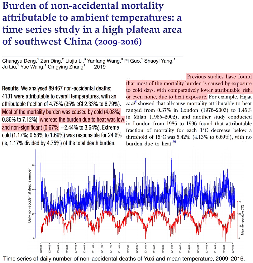
Díaz et al., 2019     Results: The results show that the RRs [relative risks/mortality due to cold weather] for Spain as a whole were 1.12 (95% CI: 1.08 1.16) for the first period [1983-1992], 1.15 (95% CI: 1.09 1.22) for the second [1993-2003] and 1.18 (95% CI: 1.10 1.26) for the third [2004-2013]. The impact of cold days has risen slightly over time, though the differences were not statistically significant. These findings show a clearly different behaviour pattern to that previously found for heat. Conclusion: The results obtained in this study do not show a downward trend for colds days [during 1983-2013]. … In the first place, here in Spain daily cold-related mortality is higher than heat-related mortality (3.5 deaths/day versus 3.0 deaths/day) (Carmona et al., 2016a). … In the case of Spain, studies conducted for the city of Madrid by age group showed heat-related mortality to be decreasing across all age groups, while cold-related mortality was increasing, particularly in the over-65 age bracket (Díaz et al., 2015b). … One study recently undertaken in the city of Madrid shows that heat-related mortality in Madrid across the period 2001–2009 accounted for 344 deaths, whereas cold-related mortality accounted for a total of 1473 deaths, i.e., fourfold that of heat.

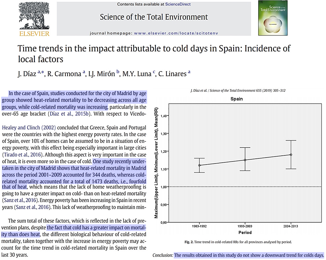
Lin et al., 2019     Temperature-related risks varied with study area and health outcome. Meta-analysis showed greater all-cause mortality risk occurred in low temperatures than in high temperatures. Integrated RR [relative risk] of all-cause mortality was 1.71 (95% confidence interval [CI]:1.43–2.04) in the 5th percentile [cold] temperature and 1.10 (95% CI: 1.05–1.15) in the 95th percentile [hot] temperature, while the lowest mortality risk was in the 60th percentile temperature (22.2 °C).

Sera et al., 2019     We collected ambient temperature and mortality daily time-series data for 340 cities in 22 countries, in periods between 1985 and 2014. … We used distributed lag non-linear and multivariate metaregression models to estimate fractions of mortality attributable to heat and cold (AF%) in each city, and to evaluate the effect modification of each indicator across cities. … Results: Heat- and cold-related deaths amounted to 0.54% (95% confidence interval: 0.49 to 0.58%) and 6.05% (5.59 to 6.36%) of total deaths, respectively.

Chu et al., 2019     We investigated the effects of cold and hot seasons on hospital admissions for acute myocardial infarction (AMI) at the junction of tropical and subtropical climate zones. … AMI hospitalizations in the cold season (cold-season-AMIs) were significantly greater than those in the hot season (OR 1.15; 95% CI 1.10–1.21). … The cold season shows increased risks for AMI, markedly among the ≥65 years cohort in the subtropical region, and among the patients diagnosed with either DM or dyslipidemia but not both in the tropical region. Age and comorbidity of metabolic dysfunction influence the season-related incidences of AMI in different climatic regions.

Åström et al., 2019     We used daily information on deaths from state death registries and minimum temperatures from November to March over the period 1997–2015 in Tallinn and 2009–2015 in Riga. The relationship between the daily minimum temperature and mortality was investigated using the Poisson regression, combined with a distributed lag non-linear model considering lag times of up to 21 days. Results: We found significantly higher all-cause mortality owing to cold temperatures both in Tallinn (Relative Risk (RR) = 1.28, 95% Confidence Interval (CI) 1.01–1.62) and in Riga (RR = 1.41, 95% CI 1.11–1.79). In addition, significantly increased mortality due to cold temperatures was observed in the 75+ age group (RR = 1.64, 95% CI 1.17–2.31) and in cardiovascular mortality (RR = 1.83, 95% CI 1.31–2.55) in Tallinn and in the under 75 age group in Riga (RR = 1.58, 95% CI 1.12–2.22).

No Increasing Trends In Intense Storms, Hurricanes

Gertler and O’Gorman     The circulation of the Northern Hemisphere extratropical troposphere has changed over recent decades [1979-2017], with marked decreases in extratropical cyclone activity and eddy kinetic energy (EKE) in summer and increases in the fraction of precipitation that is convective in all seasons. Decreasing EKE in summer is partly explained by a weakening meridional temperature gradient, but changes in vertical temperature gradients and increasing moisture also affect the mean available potential energy (MAPE), which is the energetic reservoir from which extratropical cyclones draw. … These results connect changes in the atmospheric mean state with changes in both large-scale and convective circulations, and they suggest that extratropical cyclones can weaken even as their associated convection becomes more energetic.

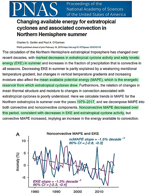
Trenary et al., 2019     The impact of anthropogenic forcings on tropical North Atlantic hurricane potential intensity (PI) is evaluated in CMIP5 models for the period 1958‐2005. Eleven models are examined, but only seven models have a forced response that is distinguishable from internal variability. The use of discriminant analysis to optimize detectability does not yield a clear, common climate change signal. Of the seven models with a significant response, one has a negative linear trend while two have a positive linear trend. The trend in PI [hurricane potential intensity] is not even consistent among reanalyses, although this difference is not statistically significant because of large uncertainties. Furthermore, estimates of PI internal variability have significantly different variances among different reanalysis products. These disagreements between models, reanalysis products, and between models and reanalyses, in conjunction with relatively large uncertainties, highlight the difficulty of detecting and attributing observed changes in North Atlantic hurricane potential intensity.

Takagi, 2019     The Emergency Events Database (EM-DAT) indicates that the economic damage associated with storms has been rapidly growing in Vietnam. By contrast, the fatality rate due to storm-relevant disasters has been declining in recent decades. This study investigates whether typhoon trends have affected these outcomes. … Moreover, the analysis of variance (ANOVA) illustrates that none of the meteorological trends such as frequency, central pressure, wind speed, or storm intensity show any significant increase or decrease over the last four decades. However, landfall frequency has risen significantly, particularly in the northernmost part of the country where two large cities, Hanoi and Hai Phong, are located.

No Increasing Trend In Drought/Flood Frequency, Severity

Mishra et al., 2019     Millions of people died due to famines in India in the nineteenth and twentieth centuries; however, the relationship of historical famines with drought is complicated and not well understood. Using station‐based observations and simulations, we reconstruct soil moisture (agricultural) drought in India for the period 1870–2016. We show that over this century and a half period, India experienced seven major drought periods (1876–1882, 1895–1900, 1908–1924, 1937–1945, 1982–1990, 1997–2004, and 2011–2015) based on severity‐area‐duration analysis of reconstructed soil moisture. Out of six major famines (1873–74, 1876, 1877, 1896–97, 1899, and 1943) that occurred during 1870–2016, five are linked to soil moisture drought, and one (1943) was not. The three most deadly droughts (1877, 1896, and 1899) were linked with the positive phase of El Niño–Southern Oscillation. Five major droughts were not linked with famine, and three of those five nonfamine droughts occurred after Indian independence in 1947.

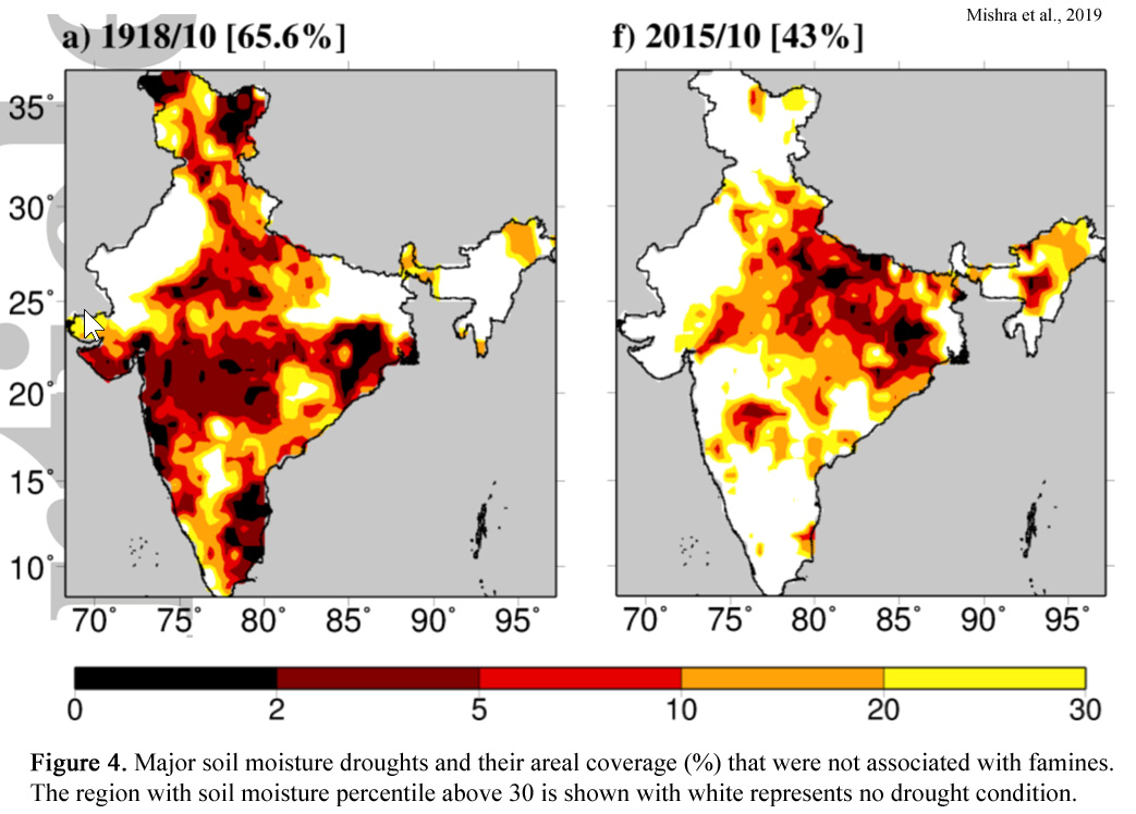
Toomey et al., 2019     Increased cold event frequency over the continental United States is often indicative of negative phases of the NAO (Thompson & Wallace, 2001), and both records above bear similarities to the 1,000‐year long NAO reconstruction of Trouet et al. (2009; Figure 4b). While the winter moisture budget (evaporation minus precipitation) over much of Eastern North America changes little between NAO phases (Hurrell, 1995), persistent weakness of the western end of the subtropical ridge—implied by more negative NAO conditions—is consistent with enhanced hurricane tracking toward the East Coast (e.g., Kossin et al., 2010). Increased hurricane rainfall may therefore explain, in part, intervals of increased flood frequency on the Susquehanna during the late Holocene as well as nearby rivers such as the Little Tennessee River, North Carolina‐Tennessee (L. Wang & Leigh, 2012), and Greenbrier River, West Virginia (Aldred, 2010). Negative NAO conditions may also foster stronger tropical cyclone genesis, overall, in the Main Development Region (~10–20° N, 20–85° W; Figure 4a). … We find more frequent deposition from large floods when Chesapeake Bay SSTs, based on Mg/Ca ostracodes measurements (Figure 4c), were colder than normal (Cronin et al., 2003, 2010).

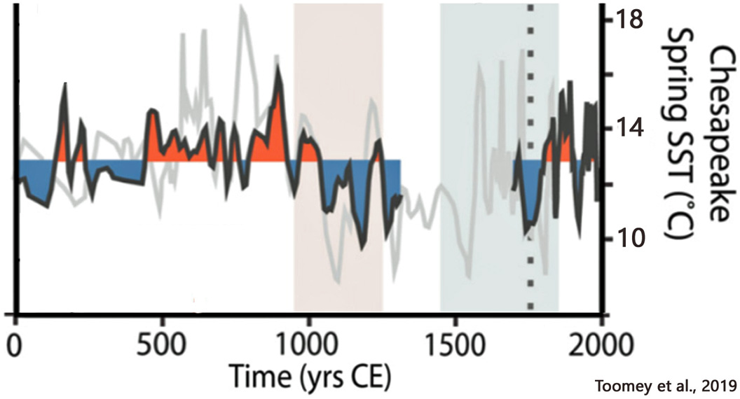
Baek et al., 2019     We examine oceanic drivers of widespread droughts over the contiguous United States (herein pan‐CONUS droughts) during the Common Era in what is one of the first analyses of the new Paleo Hydrodynamics Data Assimilation (PHYDA) product. The canonical understanding of oceanic influences on North American hydroclimate suggests that pan‐CONUS droughts are forced by a contemporaneous cold tropical Pacific Ocean and a warm tropical Atlantic Ocean. We test this hypothesis using the paleoclimate record. Composite analyses find a robust association between pan‐CONUS drought events and cold tropical Pacific conditions, but not with warm Atlantic conditions. Similarly, a self‐organizing map analysis shows that pan‐CONUS drought years are most commonly associated with a global sea surface temperature pattern displaying strong La Niña and cold Atlantic Multidecadal Oscillation (AMO) conditions. Our results confirm previous model‐based findings for the instrumental period and show that cold tropical Pacific Ocean conditions are the principal driver of pan‐CONUS droughts on annual timescales.

Formetta and Feyen, 2019     Empirical evidence of declining global vulnerability to climate-related hazards … For the period 1980–2016 we have analyzed the seven weather-related hazards: general floods, flash floods, coastal floods, cold related hazard, heatwaves, droughts, and wind related hazards. … Global average mortality and loss rates have dropped by 6.5 and nearly 5 times, respectively, from 1980 to 1989 to 2007–2016.

Natural CO2 Emissions A Net Source, Not A Net Sink

Dixit et al., 2019     The key role of oceans in the global climatic system can be accurately quantified by the measurement of CO 2 exchange across air–sea interface. The direction and magnitude of this CO 2 exchange are mainly governed by the gradient of partial pressure of carbon dioxide (pCO 2 ) at the air–sea interface. … Derived fluxes showed that BOB [Bay of Bengal] is a net annual source (0.440 g-C/m 2 /year for year 2014) of CO 2 at mooring location with significant seasonality effects.

Tian et al., 2019    The equatorial Pacific is the major source region for outgassing CO2 to the atmosphere, annually amounting to 0.44±0.14 PgC (Feely et al. 1999; Ishii et al. 2014).

Kim et al., 2019     According to a modeling study (Landschützer et al., 2016), the present study site was a very weak CO2 sink in 2003–2007, whereas it was a net source in 2008–2013 (Figure 5b). A study of CO2 exchange in the Central and Eastern Equatorial Pacific also showed stronger outgassing of CO2 during a negative PDO period (Feely et al., 2006).

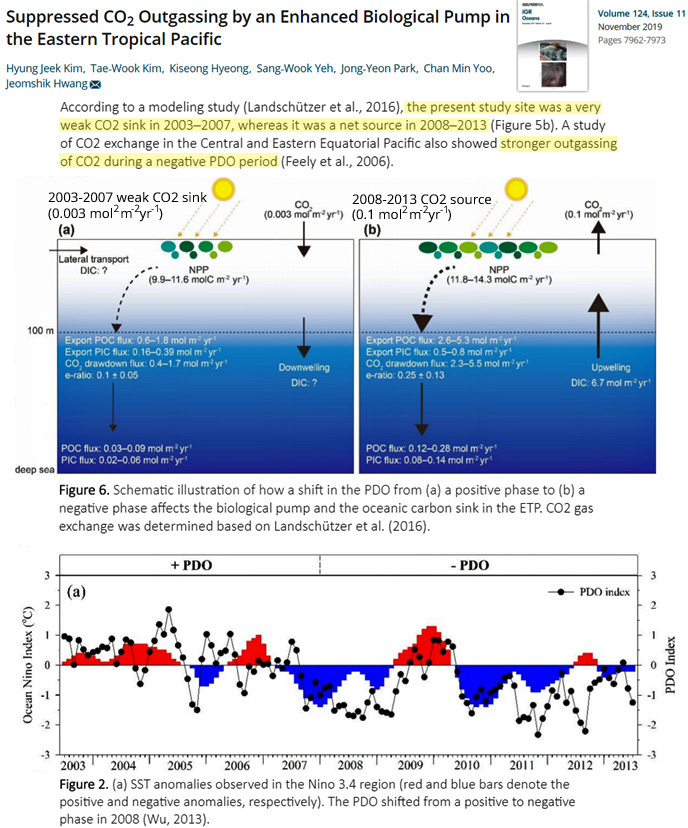
Miscellaneous

CO2 Changes Lag Warming

Muschitiello et al., 2019     Deep-water circulation changes lead North Atlantic climate during deglaciation … The analysis reveals that changes in Nordic Seas NADW [North Atlantic Deep Water] formation occurred before the climate shifts into and out of GS-1 (YD) [Younger Dryas deglaciation/warming, ~11,700 yrs before present] by 385 ± 32 (1σ bounds) and 447 ± 27 years, respectively, and that weakening of Nordic Seas NADW [North Atlantic Deep Water] occurred 437 ± 79 years prior to the first signs of pCO2 rise near the start of GS-1 (YD) [Younger Dryas deglaciation/warming, ~11,700 yrs before present] . Importantly, the latter finding substantiates the hypothesised lag between AMOC reduction and pCO2 rise during early deglaciation and is observed in climate simulations as a transient response of the global efficiency of the biological pump to AMOC slowdown.

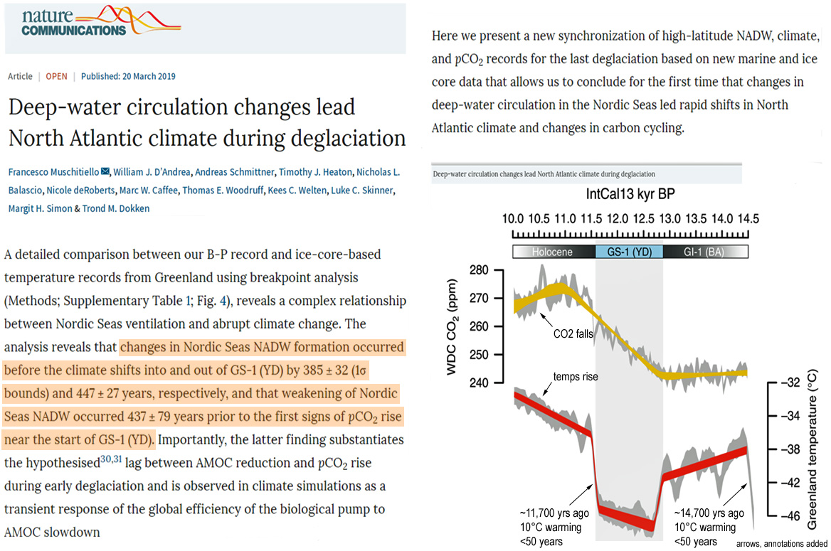
Arctic Outgoing Longwave Radiation (OLR) increasing (not decreasing)

Peterson et al., 2019    Sensitivity studies reveal that surface temperature contributes much more than atmospheric temperature and humidity to the spectral OLR and GHE trends, while the contributions from the latter two are also discernible over many spectral regions (e.g., trends in the far‐IR dirty window in March). The largest increase of spectral GHE is seen north of 80°N in March across the water vapor v2 band and far‐IR. When the secular fractional change of spectral OLR is less than that of surface spectral emission, an increase of spectral GHE can be expected. Spectral trend analyses reveal more information than broadband trend analyses alone.

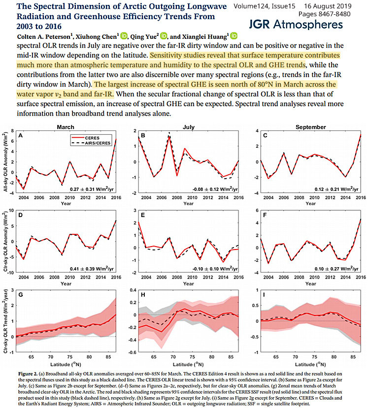
Trends in ocean heat content change and in the Earth’s Energy Imbalance are falling since 2000

Dewitte et al., 2019     The OHCTD [Ocean Heat Content Time Derivative] over the period 1960–2015 shows three different regimes, with low OHCTD prior to 1982, rising OHCTD from 1982 to 2000, and decreasing OHCTD [Ocean Heat Content Time Derivative] since 2000. These OHCTD periods correspond to periods of slow/rapid/slow surface temperature rise [16,17], to periods of strong La Ninas/El Ninos/La Ninas [14,18], and to periods of increasing/decreasing/increasing aerosol loading [19,20]. A better understanding of these past and ongoing climate changes is a necessary condition for our ability to make a skillfull prediction of future climate change. … The EEI [Earth Energy Imbalance, 2000-2018] shows a trend of −0.16 ± 0.03 (1 σ) W/m2dec. If the RSR ageing correction uncertainty (Section 4) is taken into account the uncertainty becomes ±0.11 W/m2dec. This means that the EEI seems to have a decreasing trend. At first sight it seems surprising that the EEI is decreasing during a period of continued greenhouse gas emission. … Due to the high ocean heat content, it is expected that the EEI and the OHCTD are nearly equal. From Figure 15, we can discriminate three phases in the OHCTD from 1967 to 2010: Prior to 1982, the mean value of the OHCTD is 0.071 ± 0.05 (1 σ) W/m2, the trend is −0.07 ± 0.1 (1 σ) W/m2dec. From 1982 to 2000, the OHCTD is increasing with a trend of 0.32 ± 0.05 (1 σ) W/m2dec. After 2000, the OHCTD is decreasing with a trend of −0.26 ± 0.06 (1 σ) W/m2dec. Within their uncertainties, the trends after 2000 of the EEI (−0.16 ± 0.11 W/m2dec) and of the OHCTD (−0.26 ± 0.06 (1 σ) W/m2dec), agree. This again adds extra confidence to our results.

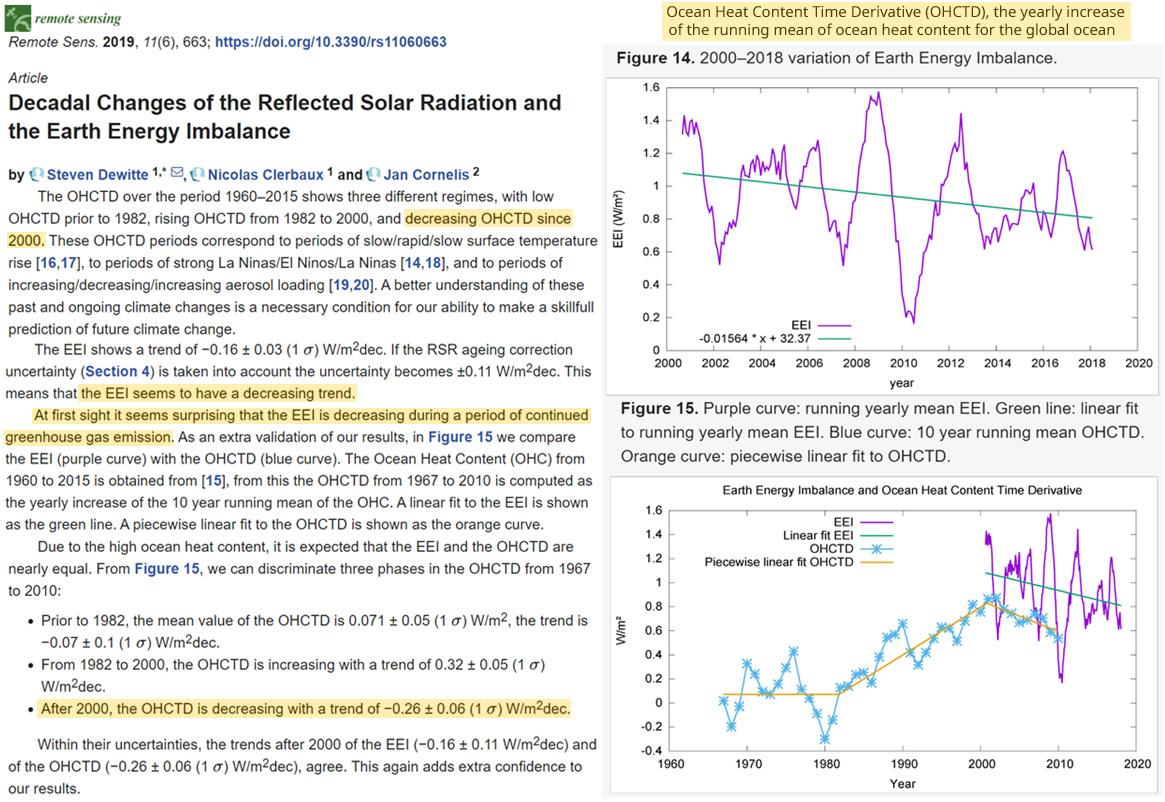
Temperature change episodes of greater magnitude and duration than modern

Allan et al., 2019     Importantly, while Niño 4 SST anomalies recorded during the austral summer of 2016 were the highest values on record, an analysis of long-term palaeoclimate records indicates that there may have been episodes of greater magnitude and duration than seen in instrumental observations.

Upwelling long-wave (not downwelling) dominates long-wave energy transfer for water bodies

Solcerova et al., 2019     The skin effect refers to a thin, more or less stable layer of surface water that is colder than the water beneath it due to radiative energy loss that exceeds the replenishment of energy via shortwave absorption or thermal diffusion from the lower water. As the energy transfer from water to atmosphere (evaporation, long-wave radiation, or sensible heat) happens at the surface, a thin cold layer is created (the skin effect). In natural lakes, the upwelling long-wave radiation dominates long-wave energy transfer. This is due to the surface supplying all outgoing long-wave energy, while incoming shortwave energy is absorbed through the first meters of the water column. The thickness of the skin layer is hypothesised to be regulated by conductive and diffusive heat processes. … Our data suggest that the skin effect of fresh water bodies is predominantly a daytime phenomenon and only occurs during low to zero wind speeds.

[CO2 and downwelling long-wave radiation are not mentioned anywhere in the paper as a mechanistic factor in water temperature changes.]

Peak Oil as a “wrong and misleading” concept

Bardi, 2019     Today, 20 years have passed since the publication of the ground-breaking Scientific American report [1]. The expected world peak has not arrived, at least in terms of a reduction of the global supply of liquid fuels [11] and, in general, the concept of peak oil has faded from the mainstream discussion as well as from the scientific literature. ASPO international seems to have disappeared as an active association around 2012–2013, although some national branches of the association still exist. The generally accepted explanation for the fading interest in the concept attributes it to the “wrong predictions” of the date of the peak and, from there, most mainstream reports tend to define the whole concept  as wrong and misleading.

Atmospheric CO2 follows temperature change

Jacobs and Preat, 2019     Geology thus shows us not only that the temperature was often much higher on Earth than today’s, but also that the CO2 content in the atmosphere was higher, usually more than 5 (Mesozoic ) at 25 (Paleozoic) times the current, or even 100 to 1000 times higher in Precambrian. For the proponents of the hypothesis of the greenhouse effect, the conclusion is obvious: it is the gases CH4 and / or CO2 (also N2O?) which caused the reheating of the past. How to be sure? This is the whole question, and we will see here that thanks to fairly precise magnetoand bio-stratigraphic temporal resolutions coupled with a cyclostratigraphy related to orbital forcing of the Earth, the opposite has occurred, know that CO2 follows the increase in temperature.

CO2 concentrations naturally higher (756 ppm) in winter (caves)?

Al-Manmi et al., 2019     Calcite growth at site 1 reflects a seasonal growth pattern in which higher cave air CO2 concentrations inhibit CO2 degassing from cave dripwater and thus inhibit calcite precipitation. This process is driven by varying temperature gradient between surface air and cave air, which drives the ventilation of caves (Banner et al., 2007). The average cave air pCO2 is 596 ppm; in Shalaii Cave air pCO2 rises in mid-January, reaching winter values of 756 ppm and then falling to less than 484 ppm in mid–September, which is nearly atmospheric. The control on cave air pCO2 is complex; in the winter there is a rise in cave air pCO2, which is primarily a result of reversals in chimney ventilation driven by temperature being in contrast between the cave interior and exterior, with additional transient effects caused by synoptic scale atmospheric pressure and wind conditions (Mattey et al., 2008).

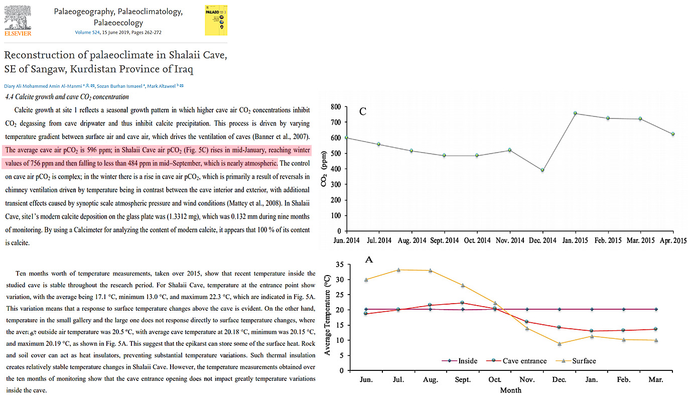
Climate sensitity to quadrupled CO2 1.88 K to 2.27 K?

Chen et al., 2019     Climate sensitivity and feedbacks are basic and important metrics to a climate system. They determine how large surface air temperature will increase under CO2 forcing ultimately, which is essential for carbon reduction policies to achieve a specific warming target. In this study, these metrics are analyzed in a climate system model newly developed by the Chinese Academy of Meteorological Sciences (CAMS-CSM) and compared with multi-model results from the Coupled Model Comparison Project phase 5 (CMIP5). Based on two idealized CO2 forcing scenarios, i.e., abruptly quadrupled CO2 and CO2 increasing 1% per year, the equilibrium climate sensitivity (ECS) and transient climate response (TCR) in CAMS-CSM are estimated to be about 2.27 and 1.88 K, respectively. The ECS is near the lower bound of CMIP5 models whereas the TCR is closer to the multi-model ensemble mean (MME) of CMIP5 due to compensation of a relatively low ocean heat uptake (OHU) efficiency. The low ECS is caused by an unusually negative climate feedback in CAMS-CSM, which is attributed to cloud shortwave feedback (λSWCL) over the tropical Indo-Pacific Ocean.