I. Lack Of Anthropogenic/CO2 Signal In Sea Level Rise (34)
Donchyts et al., 2016 Earth’s surface water change over the past 30 years [1985-2015] … Earth’s surface gained 115,000 km2 of water and 173,000 km2 of land over the past 30 years, including 20,135 km2 of water and 33,700 km2 of land in coastal areas. [A net decline in water on the Earth’s surface relative to land, including across the Earth’s coastal regions.]
(press release) Coastal areas were also analysed, and to the scientists surprise, coastlines had gained more land – 33,700 sq km (13,000 sq miles) – than they had been lost to water (20,100 sq km or 7,800 sq miles). … “We expected that the coast would start to retreat due to sea level rise, but the most surprising thing is that the coasts are growing all over the world,” said Dr Baart. “We’re were able to create more land than sea level rise was taking.” … The researchers said Dubai’s coast had been significantly extended, with the creation of new islands to house luxury resorts. “China has also reconstructed their whole coast from the Yellow Sea all the way down to Hong Kong,” said Dr Baart.
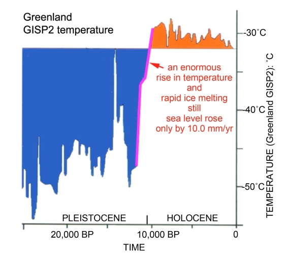
Mörner, 2016 Sea level is globally varying between ±0.0 and +1.0 mm/yr (0.5 ± 0.5 mm/yr). … At 11,000 BP we had enormous amounts of ice still left in the huge continental ice caps of the Last Ice Age. In Canada, the ice front was in St. Lawrence lowland, and in Scandinavia, the ice margin was at Stockholm. At the warming pulse ending the Pleistocene and starting the Holocene, ice melted at an exceptionally strong forcing. Today, there is neither ice nor climate forcing that in any way can be compared to what happened 11,000 – 10,000 BP. The conclusion is obvious; we can never in present time have any ice melting and sea level rise as strong- and certainly not stronger-than that occurring at the Pleistocene/Holocene transition. Therefore, a rate of sea level rise of +10.0 mm/yr or 1.0 m per century can be held as the absolutely ultimate value of any present day sea level rise. Any present rise in sea level must be far below this value to be realistic in view of past records and the physical factors controlling ice melting. Therefore, we can also dismiss any claim of sea level rise exceeding 1 m in the next century as sheer nonsense and unfounded demagoguery.
Hadi Bordbar et al., 2016 The tropical Pacific has featured some remarkable trends during the recent decades such as an unprecedented strengthening of the Trade Winds, a strong cooling of sea surface temperatures (SST) in the eastern and central part, thereby slowing global warming and strengthening the zonal SST gradient, and highly asymmetric sea level trends with an accelerated rise relative to the global average in the western and a drop in the eastern part. These trends have been linked to an anomalously strong Pacific Walker Circulation, the major zonal atmospheric overturning cell in the tropical Pacific sector, but the origin of the strengthening is controversial. Here we address the question as to whether the recent decadal trends in the tropical Pacific atmosphere-ocean system are within the range of internal variability, as simulated in long unforced integrations of global climate models. We show that the recent trends are still within the range of long-term internal decadal variability. Further, such variability strengthens in response to enhanced greenhouse gas concentrations, which may further hinder detection of anthropogenic climate signals in that region.
Palanisamy, 2016 Building up on the relationship between thermocline and sea level in the tropical region, we show that most of the observed sea level spatial trend pattern in the tropical Pacific can be explained by the wind driven vertical thermocline movement. By performing detection and attribution study on sea level spatial trend patterns in the tropical Pacific and attempting to eliminate signal corresponding to the main internal climate mode, we further show that the remaining residual sea level trend pattern does not correspond to externally forced anthropogenic sea level signal. In addition, we also suggest that satellite altimetry measurement may not still be accurate enough to detect the anthropogenic signal in the 20-year tropical Pacific sea level trends.
Hansen et al., 2016 Together with a general sea-level rise of 1.18 mm/y, the sum of these five sea-level oscillations constitutes a reconstructed or theoretical sea-level curve of the eastern North Sea to the central Baltic Sea, which correlates very well with the observed sea-level changes of the 160-year period (1849–2009), from which 26 long tide gauge time series are available from the eastern North Sea to the central Baltic Sea. Such identification of oscillators and general trends over 160 years would be of great importance for distinguishing long-term, natural developments from possible, more recent anthropogenic sea-level changes. However, we found that a possible candidate for such anthropogenic development, i.e. the large sea-level rise after 1970, is completely contained by the found small residuals, long-term oscillators, and general trend. Thus, we found that there is (yet) no observable sea-level effect of anthropogenic global warming in the world’s best recorded region.
Mörner, 2016 Coastal erosion is caused by many different processes like changes in prevailing wind direction, coastal currents, re-establishment of a new equilibrium profile, sea level rise, sea level fall, exceptional storms, hurricanes/cyclones, and tsunami events. These coastal factors are reviewed with special attention to effects due to changes in sea level. In the Indian Ocean, sea level seems to have remained virtually stable over the last 40-50 years. Coastal erosion in the Maldives was caused by a short lowering in sea level in the 1970s. In Bangladesh, repeated disastrous cyclone events cause severe coastal erosion, which hence has nothing to do with any proposed sea level rise. Places like Tuvalu, Kiribati and Vanuatu – all notorious for an inferred sea level rise – have tide gauges which show no on-going sea level rise. Erosion is by no means a sign of sea level rise. Coastal erosion occurs in uplifting regions as well as in subsiding regions, or virtually stable areas. Coastal morphology provides excellent insights to the stability.
Parker and Ollier, 2016 Tide gauges provide the most reliable measurements, and best data to assess the rate of change. We show as the naïve averaging of all the tide gauges included in the PSMSL surveys show “relative” rates of rise about +1.04 mm/year (570 tide gauges of any length). If we consider only 100 tide gauges with more than 80 years of recording the rise is only +0.25 mm/year. This naïve averaging has been stable and shows that the sea levels are slowly rising but not accelerating. …The satellite altimetry returns a noisy signal so that a +3.2 mm/year trend is only achieved by arbitrary “corrections”. We conclude that if the sea levels are only oscillating about constant trends everywhere as suggested by the tide gauges, then the effects of climate change are negligible, and the local patterns may be used for local coastal planning without any need of purely speculative global trends based on emission scenarios.
Mörner, 2016 Observational facts recorded and controllable in the field tell a quite different story of actual sea-level rise than the ones based on model simulations, especially all those who try to endorse a preconceived scenario of disastrous flooding to come. “Poster sites” like Tuvalu, Vanuatu, and Kiribati in the Pacific have tide gauge stations indicating stable sea-level conditions over the last 20–30 years. The Maldives, Goa, Bangladesh, and several additional sites in the Indian Ocean provide firm field evidence of stable sea-level conditions over the last 40–50 years. Northeast Europe provides excellent opportunities to test regional eustasy, now firmly being set at +1.0 ± 0.1 mm/year. Other test areas like Venice, Guyana–Surinam, Qatar, and Perth provide a eustatic factor of ±0.0 mm/year. We now have a congruent picture of actual global sea-level changes, ie, between ±0.0 to +1.0 mm/year. This implies little or no threat for future sea-level problems.
Testut et al., 2016 We show that Grande Glorieuse Island has increased in area by 7.5 ha between 1989 and 2003, predominantly as a result of shoreline accretion [growth]: accretion occurred over 47% of shoreline length, whereas 26% was stable and 28% was eroded. Topographic transects and field observations show that the accretion is due to sediment transfer from the reef outer slopes to the reef flat and then to the beach. This accretion occurred in a context of sea level rise: sea level has risen by about 6 cm in the last twenty years and the island height is probably stable or very slowly subsiding. This island expansion during a period of rising sea level demonstrates that sea level rise is not the primary factor controlling the shoreline changes. This paper highlights the key role of non-climate factors in changes in island area, especially sediment availability and transport.
Thompson et al., 2016 Ocean dynamics, land motion, and changes in Earth’s gravitational and rotational fields cause local sea level change to deviate from the rate of global mean sea level rise. Here, we use observations and simulations of spatial structure in sea level change to estimate the likelihood that these processes cause sea level trends in the longest and highest-quality tide gauge records to be systematically biased relative to the true global mean rate. The analyzed records have an average 20th century rate of approximately 1.6 mm/yr, but based on the locations of these gauges, we show the simple average underestimates the 20th century global mean rate by 0.1 ± 0.2 mm/yr. Given the distribution of potential sampling biases, we find < 1% probability that observed trends from the longest and highest-quality TG [tide gauge] records are consistent with global mean rates less than 1.4 mm/yr.
Svendsen et al., 2016 Stable reconstruction of Arctic sea level for the 1950–2010 period … From our reconstruction, we found that the Arctic mean sea level trend is around 1.5 mm +/- 0.3 mm/y for the period 1950 to 2010, between 68ºN and 82ºN. This value is in good agreement with the global mean trend of 1.8 +/- 0.3 mm/y over the same period as found by Church and White (2004).
Fasullo et al., 2016 Is the detection of accelerated sea level rise imminent? … Global mean sea level rise estimated from satellite altimetry provides a strong constraint on climate variability and change and is expected to accelerate as the rates of both ocean warming and cryospheric mass loss increase over time. In stark contrast to this expectation however, current altimeter products show the rate of sea level rise to have decreased from the first to second decades of the altimeter era. Here, a combined analysis of altimeter data and specially designed climate model simulations shows the 1991 eruption of Mt Pinatubo to likely have masked the acceleration that would have otherwise occurred. This masking arose largely from a recovery in ocean heat content through the mid to late 1990 s subsequent to major heat content reductions in the years following the eruption. A consequence of this finding is that barring another major volcanic eruption, a detectable acceleration is likely to emerge from the noise of internal climate variability in the coming decade. [A detectable acceleration has yet to emerge.]
Parker, 2016 The sea levels of Kiribati have been stable over the last few decades, as elsewhere in the world. The Australian government funded Pacific Sea Level Monitoring (PSLM) project has adjusted sea level records to produce an unrealistic rising trend. Some information has been hidden or neglected, especially from sources of different management. The measured monthly average mean sea levels suffer from subsidence or manipulation resulting in a tilting from the about 0 (zero) mm/year of nearby tide gauges to 4 (four) mm/year over the same short time window. Real environmental problems are driven by the increasing local population leading to troubles including scarcity of water, localized sinking and localised erosion.
Dangendorf et al., 2016 The observed 20th century sea level rise represents one of the major consequences of anthropogenic climate change. However, superimposed on any anthropogenic trend there are also considerable decadal to centennial signals linked to intrinsic natural variability in the climate system. … Gravitational effects and ocean dynamics further lead to regionally varying imprints of low frequency variability. In the Arctic, for instance, the causal uncertainties are even up to 8 times larger than previously thought. This result is consistent with recent findings that beside the anthropogenic signature, a non-negligible fraction of the observed 20th century sea level rise still represents a response to pre-industrial natural climate variations such as the Little Ice Age.
Parker, 2016 The sea level rates of rise of the worldwide surveys by the Permanent Service on Mean Sea Level (PSMSL) or the United States surveys by the National Oceanic and Atmospheric Administration (NOAA) have shown stable sea level rises, with average values over hundreds of tide gauges very small, and negligible time rates of changes of these values, but eventually negative.
Holocene Sea Levels Meters Higher When CO2 Levels Much Lower
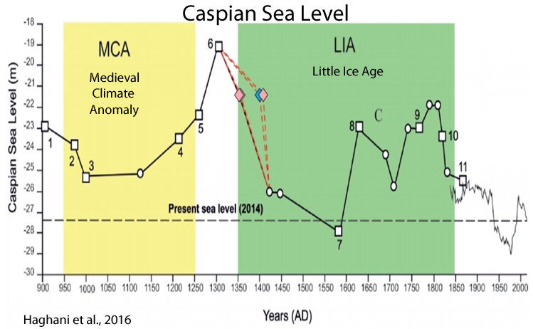
Haghani et al., 2016 Caspian Sea (CS) water level has fluctuated repeatedly with an amplitude of larger than 25m during the Holocene without any link with the eustatic sea level. During the last millennium, Caspian Sea level (CSL) experienced two significant changes: a poorly identified drop and a slightly better known rise during the Medieval Climatic Anomaly (MCA; AD 950–1250) and the ‘Little Ice Age’ (LIA; AD 1350–1850), respectively … The data from the Langarud sequence indicate that the CSL [Caspian Sea level] rose to at least −21.44m during that time (i.e. >6m higher than at present), as Langarud was probably not on the shore itself but was affected by distal brackish water flooding. This result is in line with historical findings about the CSL high-stand during the 14th and the early 15th centuries.
Zondervan, 2016 Preserved fossil coral heads as indicators of Holocene high sea level on One Tree Island [GBR, Australia] … Complete in-situ fossil coral heads have been found on beach rock of One Tree Island, a small cay in the Capricorn Group on the Great Barrier Reef. Measurements against the present low-tide mark provide a [Holocene] high stand of at least +2.85 m [above present sea levels], which can be determined in great accuracy compared to other common paleo sea-level record types like mangrove facies. The sea level recorded here is higher than most recent findings, but supports predictions by isostatic adjustment models. … Although the late Holocene high stand has been debated in the past (e.g. Belperio 1979, Thom et al. 1968), more evidence now supports a sea level high stand of at least + 1- 2 m relative to present sea levels (Baker & Haworth 1997, 2000, Collins et al. 2006, Larcombe et al. 1995, Lewis et al. 2008, Sloss et al. 2007).
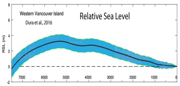
Prieto et al., 2016 Analysis of the RSL [relative sea level] database revealed that the RSL [relative sea level] rose to reach the present level at or before c. 7000 cal yr BP, with the peak of the sea-level highstand c. +4 m [above present] between c. 6000 and 5500 cal yr BP (depending on the statistical method used) or at c. 7000 cal yr BP according to the ICE-6G model prediction, gradually falling after this time to the present position … Particularly for the Río de la Plata (RDP), a Holocene RSL curve was presented by Cavallotto et al. (2004) based on 14 uncalibrated 14C ages from selected samples from the southwestern coast of the RDP (Argentina). This RSL curve was re-plotted by Gyllencreutz et al. (2010) using the same index points and qualitative approach but using the calibrated ages. It shows rising sea-levels following the Last Glacial Termination (LGT), reaching a RSL [relative sea level] maximum of +6.5 m above present at c. 6500 cal yr BP, followed by a stepped regressive trend towards the present.

Dura et al., 2016 In northern and western Sumatra, GIA models predict high rates (>5 mm/year) of RSL [relative sea level] rise from ∼12 to ∼7 ka, followed by slowing rates of rise (<1 mm/year) to an RSL [relative sea level] highstand of <1 m (northern Sumatra) and ∼3 m (western Sumatra) between 6 and 3 ka [6,000-3,000 years ago], and then gradual (<1 mm/ year) RSL fall until present.
Spotorno-Oliveira et al., 2016 At ~7000 cal. years BP the sea level in the bay [Brazil] was approximately 4 m below the present sea level and the upper subtidal benthic community was characterised by fruticose corallines on coarse soft substrate, composed mainly of quartz grains from continental runoff input. The transgressing sea rapidly rose until reaching the ~ +4 m highstand [above present] level around 5000 years BP. [Sea levels rose 8 meters in 2,000 years, or 0.4 m per century, 4 mm/year.]
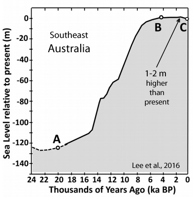
Lee et al., 2016 The configuration suggests surface inundation of the upper sediments by marine water during the mid-Holocene (c. 2–8 kyr BP), when sea level was 1–2 m above today’s level.
Yokoyama et al., 2016 The Holocene-high-stand (HHS) inferred from oyster fossils (Saccostrea echinata and Saccostrea malaboensis) is 2.7 m [above present sea level] at ca. 3500 years ago, after which sea level gradually fell to present level. The HHS magnitude attributed to GIA for the last ca. 4000 is between 1 and 1.5 m above present day sea level, and the residual indicates the long-term lithospheric uplift rate of the island. The timing of peak HHS also indicates that late Holocene melting mainly from Antarctica ceased by approximately 4000 years ago.
May et al., 2016 Beach ridge evolution over a millennial time scale is also indicated by the landward rise of the sequence possibly corresponding to the mid-Holocene sea-level highstand of WA [Western Australia] of at least 1-2 m above present mean sea level.
Hodgson et al., 2016 Rapid early Holocene sea-level rise in Prydz Bay, East Antarctica … Prydz Bay is one of the largest embayments on the East Antarctic coast and it is the discharge point for approximately 16% of the East Antarctic Ice Sheet. … The compiled geological data extend the relative sea-level curve for this region to 11,258 cal yr BP and include new constraints based on abandoned penguin colonies, new isolation basin data in the Vestfold Hills, validation of a submarine relative sea-level constraint in the Rauer Islands and recalibrated radiocarbon ages at all sites dating from 12,728 cal yr BP. The field data show rapid increases in rates of relative sea level rise of 12–48 mm/yr between 10,473 (or 9678) and 9411 cal yr BP in the Vestfold Hills and of 8.8 mm/yr between 8882 and 8563 cal yr BP in the Larsemann Hills. … The geological data imply a regional RSL [relative sea level] high stand of c. 8 m [above present levels], which persisted between 9411 cal yr BP and 7564 cal yr BP, and was followed by a period when deglacial sea-level rise was almost exactly cancelled out by local rebound.

Mann et al., 2016 Radiometrically calibrated ages from emergent fossil microatolls on Pulau Panambungan indicate a relative sea-level highstand not exceeding 0.5 m above present at ca. 5600 cal. yr BP
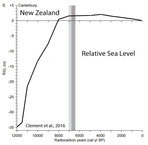
Clement et al., 2016 In North Island locations the early-Holocene sea-level highstand was quite pronounced, with RSL [relative sea level] up to 2.75 m higher than present. In the South Island the onset of highstand conditions was later, with the first attainment of PMSL being between 7000–6400 cal yr BP. In the mid-Holocene the northern North Island experienced the largest sea-level highstand, with RSL up to 3.00 m higher than present.
Long et al., 2016 RSL [relative sea level] data from Loch Eriboll and the Wick River Valley [Scotland] show that RSL [relative sea level] was <1 m above present for several thousand years during the mid and late Holocene before it fell to present.
Sander et al., 2016 Results: The data shows a period of RSL [relative sea level] highstand [Denmark] at c. 2.2 m above present MSL [mean sea level] between c. 5.0 and 4.0 ka BP [5,000 to 4,000 years before present] .After that, RSL drops by c. 1.3 m between c. 4.0 and 3.4 ka BP to an elevation roughly 1 m above present MSL. Since then, RSL has been falling at more or less even rates.
Chiba et al., 2016 Highlights: We reconstruct Holocene paleoenvironmental changes and sea levels by diatom analysis [Japan]. Average rates of sea-level rise and fall are estimated during the Holocene. Relative sea level during Holocene highstand reached 1.9 m [higher than today] during 6400–6500 cal yr BP [calendar years before present]. The timing of this sea-level rise is at least 1000 years earlier in the Lake Inba area by Holocene uplift than previous studies. The decline of sea-level after 4000 cal yr BP may correspond to the end of melting of the Antarctic ice sheet.
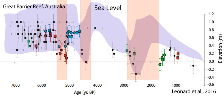
Leonard et al., 2016 Holocene sea level instability in the southern Great Barrier Reef, Australia … Three emergent subfossil reef flats from the inshore Keppel Islands, Great Barrier Reef (GBR), Australia, were used to reconstruct relative sea level (RSL). Forty-two high-precision uranium–thorium (U–Th) dates obtained from coral microatolls and coral colonies (2σ age errors from ±8 to 37 yr) in conjunction with elevation surveys provide evidence in support of a nonlinear RSL regression throughout the Holocene. RSL [relative sea level] was as least 0.75 m above present from ~6500 to 5500 yr before present (yr BP; where “present” is 1950). Following this highstand, two sites indicated a coeval lowering of RSL of at least 0.4 m from 5500 to 5300 yr BP which was maintained for ~200 yr. After the lowstand, RSL returned to higher levels before a 2000-yr hiatus in reef flat corals after 4600 yr BP at all three sites. A second possible RSL lowering event of ~0.3 m from ~2800 to 1600 yr BP was detected before RSL stabilised ~0.2 m above present levels by 900 yr BP. While the mechanism of the RSL instability is still uncertain, the alignment with previously reported RSL oscillations, rapid global climate changes and mid-Holocene reef “turn-off” on the GBR are discussed.
Wündsch et al., 2016 Compared to the present, mostly drier conditions and a greater marine influence due to a higher sea level are inferred for the period between 4210 and 2710 cal BP [calendar years before present].
Bradley et al., 2016 In general, the data [China] indicate a marked slowdown between 7 and 8 kyr BP, with sea level rising steadily to form a highstand of ~2-4 m [above present sea level] between 6 and 4 kyr BP. This is followed by a steady fall, reaching present day levels by ~1 kyr BP.

Accordi and Carbone, 2016 Then, the skeletal carbonate storage on the shelf reached its maximum 5 to 4 ka BP (Ramsay, 1995) during a highstand about 3.5 m above the present sea level [Africa], when shallow marine accommodation space was greater than at present. … A detailed sea level curve of the last 9 ka BP is reported for the Southern African coastline by Ramsay (1995), who indicates a sea level similar to that of the present (at about 6.5 ka). Ramsay also indicates successive, frequent oscillations below and above the present sea level, between a maximum of +3.5 and a minimum of -2 m. Sea level positive pulses since 7 ka BP are also documented in Siesser (1974), Jaritz et al. (1977) and Norstrom et al. (2012) for the Mozambique coast. Along the Kenyan coast, a sea level stand above the present one during the mid-Holocene is documented in many places along the coast by various authors (Hori, 1970; Toyah et al., 1973; Åse, 1981, 1987; Oosterom, 1988), where the sea level might have reached +6 m above the Kenyan Datum between 2 and 3 ka BP.

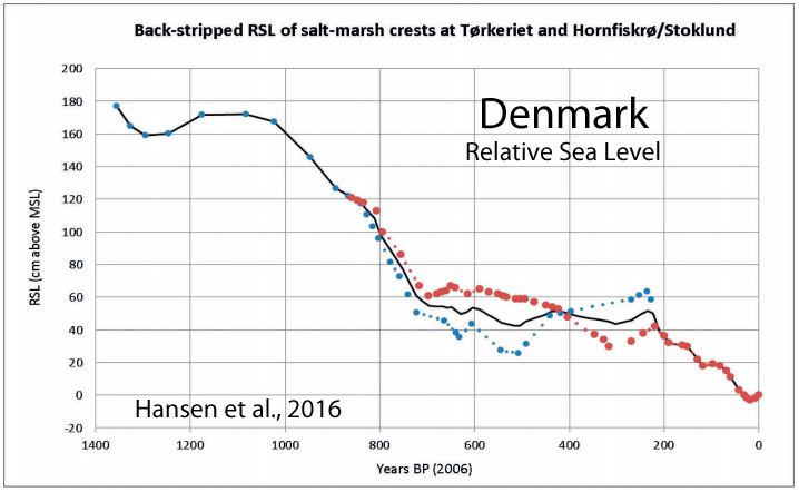
Hansen et al., 2016 Continuous record of Holocene sea-level changes [Denmark] … (4900 years BP to present). … The curve reveals eight centennial sea-level oscillations of 0.5-1.1 m superimposed on the general trend of the RSL curve
II. Warmer Holocene Climate, Non-Hockey Sticks (40)
Solomina et al., 2016 The climate was warmer and glaciers were likely receding in the beginning of the past millennium CE (the “Arkhyz break in glaciation”). … In this pass, remains of wood radiocarbon dated to 700 ± 80 BP (1180–1420 CE) were buried in a 1.5-m-thick layer of alluvium (Kaplin et al., 1971; Kotlyakov et al., 1973). Currently, the upper tree limit is located 800–900 m below this elevation. … According to indirect estimates based on pollen analyses, the upper tree limit in the “Arkhyz” period was 200–300 m higher than today (Tushinsky, Turmanina, 1979). The remains of ancient buildings and roads were also found in the Klukhorsky pass at an elevation of 2781 a.s.l. [above sea level] (Tushinsky et al., 1966), and the glacier was still present at this elevation in the mid 20th century. … [I]n Central and East Transcaucasia, there are artificial terraces at elevations where agriculture is not currently possible and that there are remnants of forests in places where forests have not grown since the 16th century Turmanina (1988), based on pollen analysis, suggested that, in the Elbrus area, the climate during the “Arkhyz” time was dryer and warmer than in the late 20th century by 1–2 °C. … Solomina et al. (2014) determined the Medieval warming in the Caucasus to be approximately 1 °C warmer than the mean of the past 4500 years. According to the Karakyol palynological and geochemical reconstructions, the warm period was long and lasted for five centuries. Considering the suggestion of Turmanina (1988) that it was also less humid, the likelihood that many glaciers, especially those located at relatively low elevation, disappeared is very high. … The maximum glacier extent in the past millennium was reached before 1598 CE. The advance of the 17th century CE, roughly corresponding to the Maunder Minimum, is recorded at Tsey Glacier. … General glacier retreat started in the late 1840s CE and four to five minor readvances occurred in the 1860s–1880s CE. In the 20th century CE, the continued retreat was interrupted by small readvances in the 1910s, 1920s and 1970s–1980s.
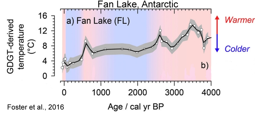
Foster et al., 2016 The Antarctic and sub-Antarctic GDGT–temperature reconstruction for Fan Lake (Fig. 5a) showed the warmest conditions between c. 3800 to 3300 cal yr BP with additional peaks in temperature at c. 2600 and 600 cal yr BP. The former was consistent with the midHolocene warm period when drier/warmer conditions prevailed on South Georgia between c. 3800 and 2800 cal yr BP seen in the Fan Lake pollen record and other records from South Georgia (e.g., Van der Putten et al., 2009).
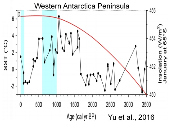
Yu et al, 2016 The period at 900–600 cal B.P. was coldest as indicated by ice advance, abundance of kill ages from ice-entombed mosses exposed recently from retreating glacial ice, and apparent gap in peatbank initiation. Furthermore, the discovery of a novel Antarctic hairgrass (Deschampsia antarctica) peatland at 2300–1200 cal B.P. from the mainland Antarctic Peninsula suggests a much warmer climate than the present. … [T]he sea surface temperature record from Palmer Deep off Anvers Island suggests a pronounced climate warming of ~3°C at 1600–500 cal B.P. [Shevenell et al., 2011].
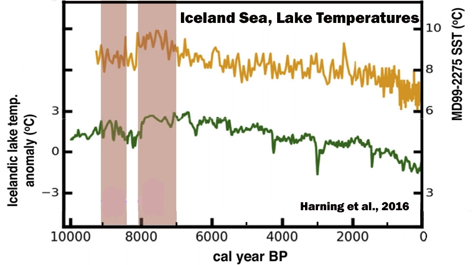
Harning et al., 2016 Distal lakes document rapid early Holocene deglaciation from the coast and across the highlands south of the glacier. Sediment from Skorarvatn, a lake to the north of Drangajokull, shows that the northern margin of the ice cap reached a size comparable to its contemporary limit by ~10.3 ka. Two southeastern lakes with catchments extending well beneath modern Drangajokull confirm that by ~9.2 ka, the ice cap was reduced to ~20% of its current area.
Otto and Roberts, 2016 In addition to temperature records limited to the past 4000 years, data for the past few thousand years were tested. When the data were explored over the past 10,000 years, greater fluctuations in the temperature can be seen with a significant rise in temperature beginning at about 11,000 BCE and ending at 2000 CE with a maximum at about 5,000 BCE.

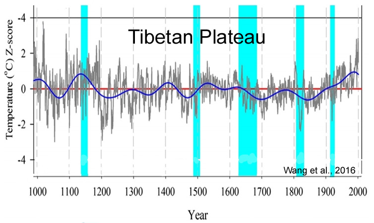
Wang et al., 2016
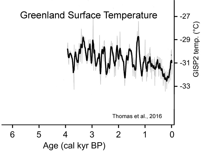
Thomas et al., 2016 Paired climate and ice sheet records from previous warm periods can elucidate the factors influencing GrIS mass balance on time scales longer than the observational record [Briner et al., 2016]. During the middle Holocene, temperature on Greenland was ~ 2°C higher than present [Cuffey and Clow, 1997; Axford et al., 2013].
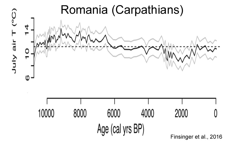
Finsinger et al., 2016
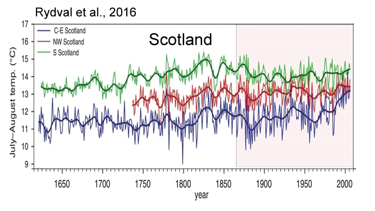
Rydval et al., 2016
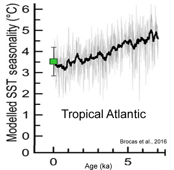
Brocas et al., 2016 [W]ithin the mid-LIG [Last Interglacial, ~125,000 years ago], a significantly higher than modern SST seasonality of 4.9°C (at 126 ka) and 4.1°C (at 124 ka) is observed. These findings are supported by climate model simulations and are consistent with the evolving amplitude of orbitally induced changes in seasonality of insolation throughout the LIG, irrespective of wider climatic instabilities that characterised this period.
Yokoyama et al., 2016 Widespread collapse of the Ross Ice Shelf during the late Holocene … The Ross Sea is a major drainage basin for the Antarctic Ice Sheet and contains the world’s largest ice shelf. Newly acquired swath bathymetry data and sediment cores provide evidence for two episodes of ice-shelf collapse. Two novel geochemical proxies, compound specific radiocarbon dating and radiogenic beryllium (10Be), constrain the timing of the most recent and widespread (∼280,000 km2) breakup as having occurred in the late Holocene. … Breakup initiated around 5 ka, with the ice shelf reaching its current configuration ∼1.5 ka. In the eastern Ross Sea, the ice shelf retreated up to 100 km in about a thousand years. Three-dimensional thermodynamic ice-shelf/ocean modeling results and comparison with ice-core records indicate that ice-shelf breakup resulted from combined atmospheric warming and warm ocean currents impinging onto the continental shelf.
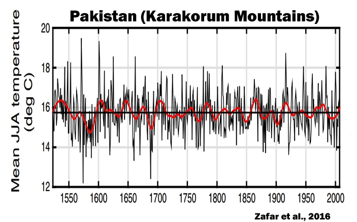
Zafar et al., 2016 [O]ur results indicate that Karakorum temperature has remained decidedly out of phase with hemispheric temperature trends for at the least the past five centuries, highlighting the long-term stability of the Karakorum Anomaly, and suggesting that the region’s temperature and cloudiness are contributing factors to the anomaly.
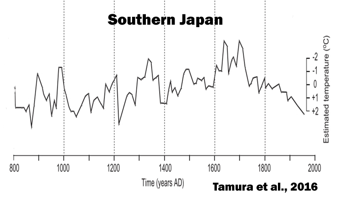
Tamura et al., 2016
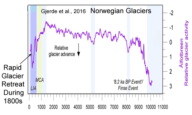
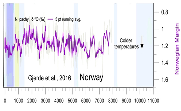
Gjerde et al., 2016 The resulting Pw record is of higher resolution than previous reconstructions from glaciers in Norway and shows the potential of glacier records to provide high-resolution data reflecting past variations in hydroclimate. Complete deglaciation of the Ålfotbreen occurred ~9700 cal yr BP, and the ice cap was subsequently absent or very small until a short-lived glacier event is seen in the lake sediments ~8200 cal yr BP. The ice cap was most likely completely melted until a new glacier event occurred around ~5300 cal yr BP, coeval with the onset of the Neoglacial at several other glaciers in southwestern Norway. Ålfotbreen was thereafter absent (or very small) until the onset of the Neoglacial period ~1400 cal yr BP. The ‘Little Ice Age’ (LIA) ~650-50 cal yr BP [1350 to 1950] was the largest glacier advance of Ålfotbreen since deglaciation, with a maximum extent at ~400-200 cal yr BP, when the ELA was lowered approximately 200 m relative to today.
Guglielmin et al., 2016 Here, we present evidence for glacial retreat corresponding to the MWP [Medieval Warm Period] and a subsequent LIA [Little Ice Age] advance at Rothera Point (67°34′S; 68°07′W) in Marguerite Bay, western Antarctic Peninsula. Deglaciation started at ca. 961–800 cal. yr BP or before, reaching a position similar to or even more withdrawn than the current state, with the subsequent period of glacial advance commencing between 671 and 558 cal. yr BP and continuing at least until 490–317 cal. yr BP. Based on new radiocarbon dates, during the MWP, the rate of glacier retreat was 1.6 m yr−1, which is comparable with recently observed rates (~0.6 m yr−1 between 1993 and 2011 and 1.4 m yr−1 between 2005 and 2011). Moreover, despite the recent air warming rate being higher, the glacial retreat rate during the MWP was similar to the present, suggesting that increased snow accumulation in recent decades may have counterbalanced the higher warming rate.
Orth et al., 2016 Our results show medium confidence that summer mean temperatures and maximum temperatures in Central Europe in 1540 were warmer than the respective present-day mean summer temperatures (assessed between 1966–2015). The model-based reconstruction suggests further that with a probability of 40%–70%, the highest daily temperatures in 1540 were even warmer than in 2003
Yu et al., 2016 We used subfossil mosses and peats to document changes in regional climate, cryosphere, and terrestrial ecosystems in the western Antarctic Peninsula at ~65°S latitude. We find that most peat-forming ecosystems have initiated since 2800 cal BP, in response to warmer summers and increasing summer insolation. The period at 900-600 cal BP [Little Ice Age] was coldest as indicated by ice advance, abundance of kill ages from ice-entombed mosses exposed recently from retreating glacial ice, and apparent gap in peatbank initiation. Furthermore, the discovery of a novel Antarctic hairgrass (Deschampsia antarctica) peatland at 2300-1200 cal BP [calendar years before present] from the mainland Antarctic Peninsula suggests a much warmer climate than the present.
Holloway et al., 2016 Several studies have suggested that sea-level rise during the last interglacial implies retreat of the West Antarctic Ice Sheet (WAIS). The prevalent hypothesis is that the retreat coincided with the peak Antarctic temperature and stable water isotope values from 128,000 years ago (128 ka) … [A] reduction in winter sea ice area of 65±7%fully explains the 128 ka ice core evidence. Our finding of a marked retreat of the sea ice at 128 ka demonstrates the sensitivity of Antarctic sea ice extent to climate warming.
Landais et al., 2016 The last interglacial period (LIG, ∼ 129–116 thousand years ago) provides the most recent case study of multimillennial polar warming above the preindustrial level and a response of the Greenland and Antarctic ice sheets to this warming, as well as a test bed for climate and ice sheet models. ;;;mHere, we provide an independent assessment of the average LIG Greenland surface warming using ice core air isotopic composition (δ 15N) and relationships between accumulation rate and temperature. The LIG [last interglacial period] surface temperature at the upstream NEEM deposition site without ice sheet altitude correction is estimated to be warmer by +8.5 ± 2.5 ◦C compared to the preindustrial period.
Rovere et al., 2016 The Last Interglacial (MIS 5e, 128-116 ka) is among the most studied past periods in Earth’s history. The climate at that time was warmer than today, primarily due to different orbital conditions, with smaller ice sheets and higher sea-level.
Molnár and Végvári, 2016 Our study provides an estimate for the value of MAT [mean annual temperature] of HTM [Holocene Thermal Maximum] of Pannon region with an interval of 0.4°C, relying on macroecological considerations. We calculate the temperature of the HTM [Holocene Thermal Maximum]1.3–1.7°C warmer than the present temperature.
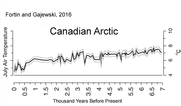
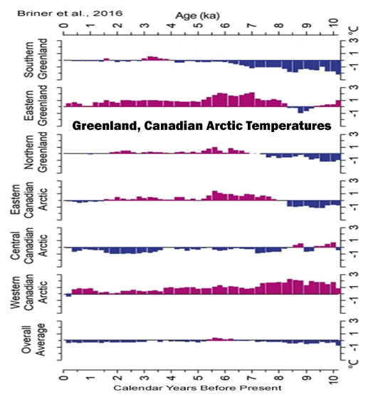
Fortin and Gajewski, 2016 A study of chironomid remains in the sediments of Lake JR01 on the Boothia Peninsula in the central Canadian Arctic provides a high-resolution record of mean July air temperatures for the last 6.9 ka …. Biological production decreased again at ~ 2 ka and the rate of cooling increased in the past 2 ka, with coolest temperatures occurring between 0.46 and 0.36 ka [460 and 360 years ago], coinciding with the Little Ice Age. Although biological production increased in the last 150 yr, the reconstructed temperatures do not indicate a warming during this time. … Modern inferred temperatures based on both pollen and chironomids are up to 3°C cooler than those inferred for the mid-Holocene.
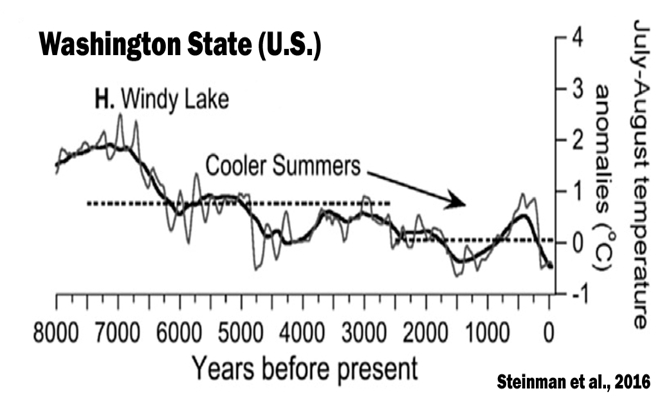
Steinman et al., 2016
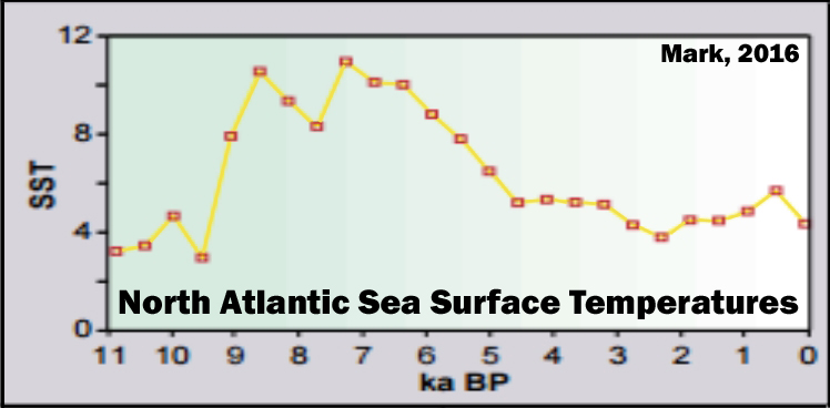
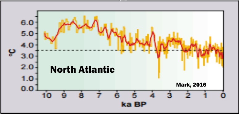
Mark, 2016 Much of the North Atlantic shows a maximum between 5000-8000 years B.P. Bradley et. al (2003) compiled a number of marine and terrestrial paleoclimatic proxies from throughout the Holocene which show fairly consistent broad trends in the climatic history of the North Atlantic region. Drawing from isotopic concentrations in ice cores, diatoms, pollen, and dendrochronological analyses, a clear period of elevated temperature, beginning at about 10,000 B.P and concluding at about 6,000 B.P precedes a slow and steady trend of cooling until present day
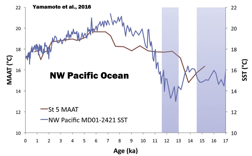
Yamamoto et al., 2016
Bradley et al., 2016 This study presehttps://notrickszone.com/wp-content/uploads/2016/12/Holocene-Cooling-Pacific-NW-Yamamoto-16.jpgnts a new model of Holocene ice-volume equivalent sea level (ESL), extending a previously published global ice sheet model (Bassett et al., 2005), which was unconstrained from 10 kyr BP to present. … The data-model misfits were examined for a large suite of ESL scenarios and a range of earth model parameters to determine an optimum model of Holocene ESL. This model is characterised by a slowdown in melting at ∼7 kyr BP [7,000 years before present], associated with the final deglaciation of the Laurentide Ice Sheet, followed by a continued rise in ESL [Holocene ice volume equivalent sea level] until ∼1 kyr BP [1,000 years before present] of ∼5.8 m associated with melting from the Antarctic Ice Sheet.
Briner et al., 2016 The temperature decrease from the warmest to the coolest portions of the Holocene is 3.0 ± 1.0 °C on average (n = 11 sites). The Greenland Ice Sheet retracted to its minimum extent between 5 and 3 ka [5,000 and 3,000 years ago], consistent with many sites from around Greenland depicting a switch from warm to cool conditions around that time. … The temperature record, which integrates all seasons, shows rapid warming from the onset of the Holocene until ~9.5 ka [9,500 years ago], relatively uniform temperature at the millennial scale until ~7 ka [7,000 years ago], followed by ~3.5 °C temperature decline to the Little Ice Age [1250-1850 C.E.], followed by ~1.5 °C warming to today. [Today’s Greenland Ice Sheet temperatures are 2.0 °C colder than the Early and Middle Holocene] . The record also shows centennial-scale variability on the order of 1-2 °C, and a ~3 °C temperature oscillation during the 8.2 ka event.

Sun et al., 2016 Here, the coexistence approach (CA) wahttps://notrickszone.com/wp-content/uploads/2016/12/Holocene-Cooling-Greenland-Ice-Sheet-Briner-16-copy.jpgs applied, and the result showed that the mean annual temperature (MAT) was about 14.8°C, and the annual precipitation (AP) was about 831.1 mm in the Guanzhong Basin during 6200–5600 cal. a BP. Comparing the climate between the mid-Holocene and present in the Xi’an area, the MAT [mean annual temperature] was about 1.1°C higher than today and the AP [annual precipitaion] was about 278 mm higher than today, similar to the modern climate of the Hanzhong area in the southern Qinling Mountains.
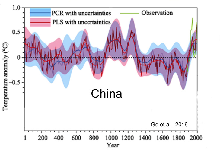
Ge et al., 2016 Results of this study show that warm intervals over the last 2000 years were in AD 1-200, AD 551-760, AD 951-1320, and after AD 1921, while cold intervals were in AD 201-350, AD 441-530, AD 781-950, and AD 1321-1920. Interestingly, temperatures during AD 981-1100 and AD 1201-1270 were comparable to those of our Present Warm Period, but have an uncertainty of 0.28°-0.42°C at 95% confidence level. Temperature variations over the whole of China are typically in phase with those of the Northern Hemisphere (NH) after AD 1000, the period which covers the Medieval Climate Anomaly, the Little Ice Age (LIA), and the Present Warm Period.
Lécuyer et al., 2016 During the ‘Green Sahara event’, water bodies developed throughout the Sahara and Sahel, reflecting the enhanced influence of the Atlantic monsoon rainfall. Major lakes then dried out between 6.5 and 3.5 ka [6,500 and 3,500 years ago]. This study investigates land cover change and lacustrine environment during the Holocene at I-n-Atei, Southern Algeria, a desert region lying in the hyperarid core of the Sahara. This site is remarkable by its extent (up to 80 km2) and by the exceptional preservation and thickness of the lacustrine deposits (7.2 m). I-n-Atei was a lake from 11 to 7.4 ka [11,000 to 7,400 years ago], then it dried out and left place to a swampy environment. … The replacement of C3 by C4 plants occurred in two main steps: a mixed C3–C4 vegetation of “wooded grassland” type was present from 10 ka to 8.4 ka while a C4 exclusive vegetation developed after 8.4 ka. After the end of the lacustrine phase a catastrophic event (flooding?) provoked the lifting of most of the lacustrine deposits and their re-deposition above the lacustrine sequence.
Nielsen et al., 2016 Here we present the first high-resolution late-Holocene glacier record from the Lofoten archipelago in northern Norway. … AMS radiocarbon dating reveals that the lake sediment record covers the last 1200 years, thereby including both the ‘Little Ice Age’ (LIA) and the ‘Medieval Climate Anomaly’ (MCA). …We found that both MCA and LIA were periods of substantial glacier variations with respect to the present, with a maximum lowering of the ELA of ~75 and ~85 m, respectively. Increased precipitation during these intervals, associated with more frequent and/or intense winter storms, is suggested to be the major driving force of glacier fluctuations in Lofoten.
Stap et al., 2016 During the past five million yrs, benthic δ18O records indicate a large range of climates, from warmer than today during the Pliocene Warm Period to considerably colder during glacials. Antarctic ice cores have revealed Pleistocene glacial–interglacial CO2 variability of 60–100 ppm, while sea level fluctuations of typically 125 m are documented by proxy data. … Our model shows CO2concentrations of 300 to 470 ppm during the Early Pliocene [~5 million years ago]. Furthermore, we simulate strong CO2 variability during the Pliocene and Early Pleistocene. These features are broadly supported by existing and new δ11B-based proxy CO2 data, but less by alkenone-based records. The simulated concentrations and variations therein are larger than expected from global mean temperature changes. Our findings thus suggest a smaller Earth System Sensitivity [to CO2 variations] than previously thought.
Belle et al., 2016 The climate evolution over the last 1400 years was marked by alternating warm and cold phases. Two main climate periods can be highlighted: the Medieval Warm Period (MWP) and the Little Ice Age (LIA). The MWP is characterized by relatively high temperatures associated with low variability (0.34 C ± 0.37). This period occurred between ca. AD 750 and ca. AD 1200. The LIA constitutes a cold period (-0.11 C ± 0.49) from ca. AD 1200 to ca. AD 1900. The end of the LIA seems late using this study, but it is still agree with several references (Millet et al. 2009; Magny et al. 2011; Luoto 2012). In the climate reconstruction provided by Guiot et al. 2010), two particular phases can be identified in this zone. The first (from ca. AD 1200 to ca. AD 1600) is clearly colder than the second. An abrupt warming appears to occur at AD 1600 during the LIA cold period. Before AD 750, the climate appears to correspond to a cold period, whereas after AD 1900, the climate corresponds to a warming period (0.04 C ± 0.49).
Paus and Haugland, 2016 The result of 344 radiocarbon-dated megafossils is here presented and discussed. This study aims at elucidating early- to mid-Holocene forest-line and climate dynamics in the southern Scandes along a present gradient of decreasing forest-line elevations. Around 9.5 calibrated ka before present (BP), pine suddenly established vertical belts of at least 200 m. These represent the highest pine-forests during the Holocene, ca. 210–170 m higher than today when corrected for land uplift. By this, summer temperatures at least 1–1.3°C warmer than today are indicated for the early Holocene thermal maximum around 8.5–9.5 cal. ka BP.
Lundeen and Brunelle, 2016 The vegetation and fire history of the Bear River Range (BRR), Southeast Idaho has been reconstructed from pollen, plant macrofossils, and macroscopic charcoal from lacustrine sediments. … Together, the proxies suggest that the early Holocene experienced larger than average snowpacks but very warm summers. Warmer than modern summer temperatures were maintained through much of the mid-Holocene, but snowpacks decreased dramatically, creating the most extreme xeric conditions in the Holocene between ~7100 and 6000 BP. After 6000 BP, summers began to show a consistent cooling trend.
Kawahata et al., 2016 During the last two millennia, SSTs fluctuated by 4.9 °C before 20 century, reaching two maximum in 1820 AD (22.3°C) and 760 AD (22.0 °C) and two minima around 145 AD (17.4 °C) and 1080 AD (17.4 °C). … Because several factors, including external forcing (e.g., solar activity) and internal forcing (e.g., volcanic activity, ENSO, and the Asian monsoon), can affect the climate, we compared SST fluctuations with each of those factors. The fluctuations cannot be explained by a single cause. It is likely that more than one driver, whether external or internal, caused the fluctuations.
Easterbrook, 2016 In the past 500 years, Greenland temperatures have fluctuated back and forth between warming and cooling about 40 times, with changes every 25–30 years. Among the more prominent climate changes recorded in the ice cores are 8500 years of Holocene temperatures that were 2–5°F warmer than present; a 8200-year cold period in the early Holocene; the Minoan Warm Period (∼3300 years ago); the Roman Warm Period (250 BC to 400 AD); the Dark Ages Cold Period (∼400–900 AD); the Medieval Warm Period (900–1300 AD); the Little Ice Age (1300 AD to the 20th century); the Wolf Minimum Cold Period (∼1280–1350 AD); the Spörer Cold Period (1460–1550 AD); the Maunder Minimum Cold Period (1645–1710); the Dalton Cold Period (1790–1820); the 1880–1915 Cold Period; the 1915–1945 Warm Period; the 1945–1977 Cold Period; and the 1978–2000 Warm Period. Comparisons of the intensity and magnitude of past warming and cooling climate changes show that the global warming experienced during the past century pales into insignificance when compared to the magnitude of profound climate reversals over the past 25,000 years. At least three warming events were 20–24 times the magnitude of warming over the past century, and four were 6–9 times the magnitude of warming over the past century. The magnitude of the only modern warming that might possibly have been caused by CO2 (1978–2000) is insignificant compared to the earlier periods of warming.
Méheust et al., 2016 [R]econstruction of sea-ice variability in the western North Pacific and Bering Sea during the past 18,000 years … The results indicate that a seasonal sea-ice cover existed during cold periods (Heinrich Stadial 1 and Younger Dryas), whereas during warmer intervals (Bølling-Allerød and Holocene) reduced sea ice or ice-free conditions prevailed in the study area. The variability in sea-ice extent seems to be linked to climate anomalies and sea-level changes controlling the oceanographic circulation between the subarctic Pacific and the Bering Sea, especially the Alaskan Stream injection though the Aleutian passes.
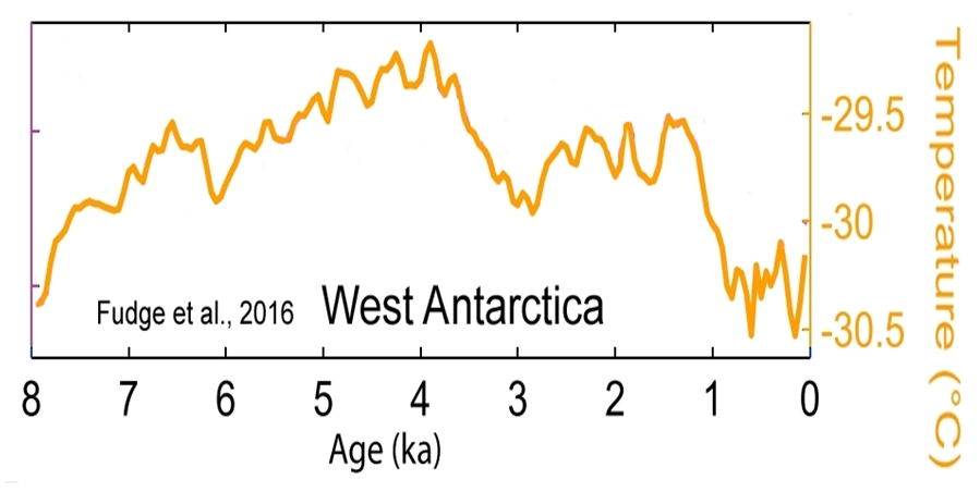
Fudge et al., 2016 The Antarctic contribution to sea level is a balance between ice loss along the margin and accumulation in the interior. Accumulation records for the past few decades are noisy and show inconsistent relationships with temperature. We investigate the relationship between accumulation and temperature for the past 31 ka using high-resolution records from the West Antarctic Ice Sheet (WAIS) Divide ice core in West Antarctica. Although the glacial-interglacial increases result in high correlation and moderate sensitivity for the full record, the relationship shows considerable variability through time with high correlation and high sensitivity for the 0–8 ka period but no correlation for the 8–15 ka period. This contrasts with a general circulation model simulation which shows homogeneous sensitivities between temperature and accumulation across the entire time period. These results suggest that variations in atmospheric circulation are an important driver of Antarctic accumulation but they are not adequately captured in model simulations. Model-based projections of future Antarctic accumulation, and its impact on sea level, should be treated with caution.
Thirumalai et al., 2016

Spolaor et al., 2016 We report bromine enrichment in the Northwest Greenland Eemian NEEM ice core since the end of the Eemian interglacial 120,000 years ago, finding the maximum extension of first-year sea ice occurred approximately 9,000 years ago during the Holocene climate optimum, when Greenland temperatures were 2 to 3 °C above present values.
(press release) Researchers have found that 8000 years ago the Arctic climate was 2 to 3 degrees warmer than now, and that there was also less summertime Arctic sea ice than today.
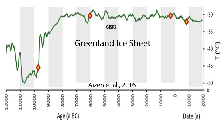
Aizen et al., 2016 [R]ecent air temperatures (1993–2003) are, on average, 0.5 °C lower than air temperatures estimated during the MWP [Medieval Warm Period] and Holocene Climate Optimum. … [P]eriods warmer than modern periods occurred for ∼6.5 ka [6,500 years] including during the HCO and Medieval Warm Period.
III. No Net Regional Warming Since Early- Mid-20th Century (15)
Christy and McNider, 2016 Three time series of average summer daily maximum temperature (TMax JJA) are developed for three interior regions of Alabama (AL) from stations with varying periods-of-record and unknown inhomogeneities. The time frame is 1883-2014. … Varying the parameters of the construction methodology creates 333 time series with a central trend-value based on the largest group of stations of -0.07 °C decade-1 with a best-guess estimate of measurement uncertainty being -0.12 to -0.02 °C decade-1. This best-guess result is insignificantly different (0.01 C decade-1) from a similar regional calculation using NOAA nClimDiv data beginning in 1895. … Finally, 77 CMIP-5 climate model runs are examined for Alabama and indicate no skill at replicating long-term temperature and precipitation changes since 1895.

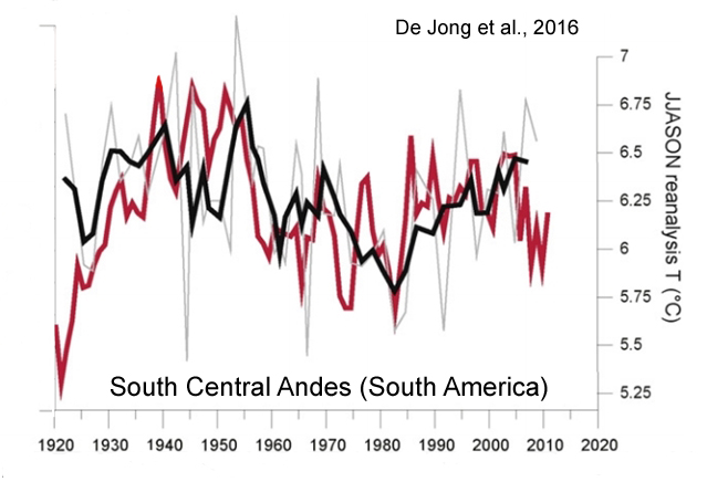
De Jong et al., 2016 [T]he reconstruction…shows that recent warming (until AD 2009) is not exceptional in the context of the past century. For example, the periods around AD 1940 and from AD 1950–1955 were warmer. This is also shown in the reanalysis data for this region and was also observed by Neukom et al. (2010b) and Neukom and Gergis (2011) for Patagonia and central Chile. Similarly, based on tree ring analyses from the upper tree limit in northern Patagonia, Villalba et al. (2003) found that the period just before AD 1950 was substantially warmer than more recent decades.
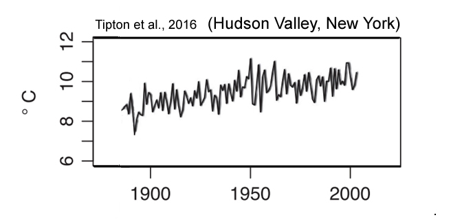
Tipton et al., 2016
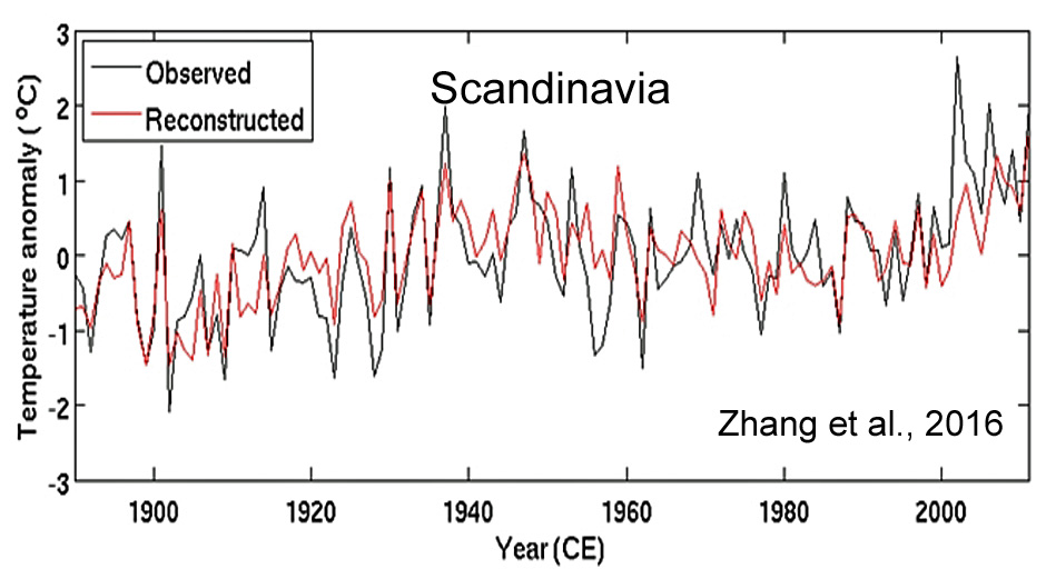
Zhang et al., 2016 [P]resent-day global mean air temperatures may have been equally high around 1000 years ago during the so-called Medieval Climate Anomaly (MCA; Lamb, 1969; Grove and Switsur, 1994). However, since regional temperature reconstructions display large variability in the timing and magnitude of the MCA (PAGES 2k Consortium, 2013), this issue has not yet been adequately settled. Hence, there is still a great need to produce and improve empirical proxy data to further our understanding of near and distant climate changes.
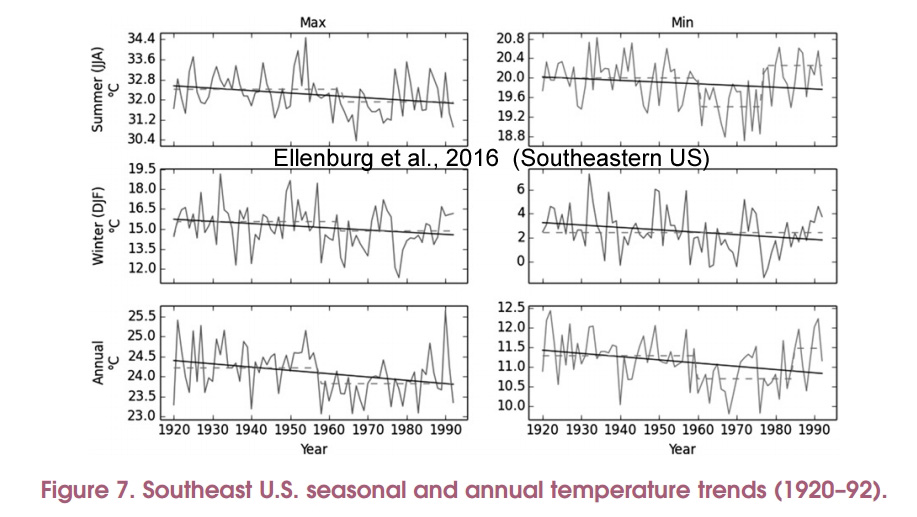
Ellenburg et al., 2016
O’Donnell et al., 2016
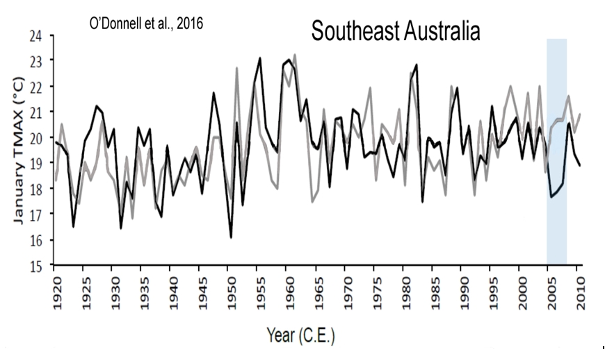
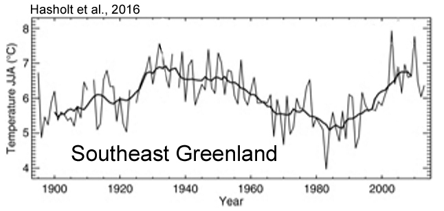
Hasholt et al., 2016 We determined that temperatures for the ablation measurement periods in late July to early September were similar in both 1933 and the recent period [1990s – present], indicating that the temperature forcing of ablation within the early warm period and the present are similar. Therefore it is reasonable to compare ARs [acceleration rates] and DDFs [degree-day factor] from 1933 with recent values, which have increased by an average of 43% and 61%, respectively. Since temperatures are not dissimilar, the increased DDFs [degree-day factors] are caused by increased ARs [degree-day factors], which must be due to changes in an energy flux that is not directly dependent on air temperature, solar radiation being the most plausible candidate. For instance, we theorize that the glacier retreat causes the termini to move to a higher altitude above the sea, reducing the shading by often-present low-level fog and thus increasing solar radiation absorption.
Chattopadhyay and Edwards, 2016 Variation in quantities such as precipitation and temperature is often assessed by detecting and characterizing trends in available meteorological data. The objective of this study was to determine the long-term trends in annual precipitation and mean annual air temperature for the state of Kentucky. Non-parametric statistical tests were applied to homogenized and (as needed) pre-whitened annual series of precipitation and mean air temperature during 1950–2010. Significant trends in annual precipitation were detected (both positive, averaging 4.1 mm/year) for only two of the 60 precipitation-homogenous weather stations (Calloway and Carlisle counties in rural western Kentucky). Only three of the 42 temperature-homogenous stations demonstrated trends (all positive, averaging 0.01 °C/year) in mean annual temperature … [B]roadly speaking, mean annual temperatures in Kentucky have not demonstrated a statistically significant trend with regard to time [during 1950-2010].
Heller, 2016 Historical data has been systematically altered over the past 15 years to cool past temperatures and increase more recent temperatures. The amount of warming from 1880 to 2000 is now shown by NASA as double what was shown in 2001. Going back further to the 1975 National Academy of Sciences report, we see a completely different story—where all 1900–40 warming was lost by 1970.
Andrews et al., 2016 Long-term observations of increasing snow cover in the western Cairngorms [Scotland] … For 13 consecutive winters between 2002 and 2015, the date for the onset of continuous winter snow cover, and subsequent melt, was recorded on slopes of north and north-easterly aspect at altitudes between 450m and 1111m amsl. Results show that the period of time during which snow is continuously present in the catchment has increased significantly by 81 (±21.01) days over the 13-year period, and that this is largely driven by a significantly later melt date, rather than earlier onset of winter snow cover.
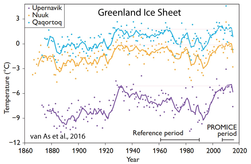
van As et al., 2016 [I]n southern Greenland ablation peaked significantly around 1930. While most of Greenland underwent relatively warm (summer) conditions in the 1930s (Cappelen 2015), this was most notable at the more southern locations, resulting in amplified ablation values according to our estimates. JJA [summer] temperatures were higher in 1928 and 1929 than in any other year of the Qaqortoq record, both attaining values of 9.2°C. This suggests that ablation in those years may have exceeded the largest net ablation measured on the Greenland ice sheet ( 2010).
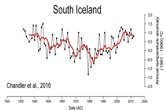
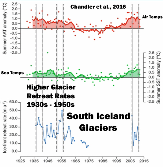
Chandler et al., 2016 [W]e calculated ice-frontal retreat rates [Skálafellsjökull glacier, SE Iceland] since the 1930s. From the calculated record of ice-front retreat, we recognised two pronounced periods of glacier recession [1936-’41 and 1951-’56] for comparison with the most recent phase of retreat (2006–2011). We undertook quantitative analysis to examine variability between these three periods of retreat, and showed that they are comparable both in style and magnitude. Analysis of climate data for SE Iceland also indicates that the three periods of ice-frontal retreat [1936-’41, 1951-’56, and 2006-’11] identified are associated with similar summer air temperature values, which has previously been shown to be a key control in terminus variations in Iceland. We, therefore, demonstrated that the coincidence of the most recent phase of ice-frontal retreat at Skálafellsjökull (2006–2011) and warming summer temperatures is not unusual in the context of the last ~80 years. This highlights the need to place observations of contemporary glacier change in a broader, longer-term (centennial) context.
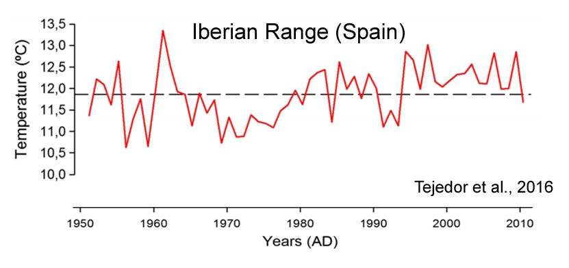
Tejedor et al., 2016
Riser et al., 2016 Most regions of the world ocean are warmer in the near-surface [0-700 m] layer than in previous decades, by over 1° C in some places. A few areas, such as the eastern Pacific from Chile to Alaska, have cooled by as much as 1° C, yet overall the upper ocean has warmed by nearly 0.2° C globally since the mid-twentieth century.
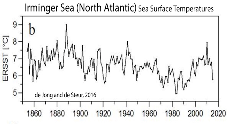
de Jong and de Steur, 2016
IV. Abrupt, Degrees-Per-Decade Natural Global Warming (Dansgaard-Oeschger Events) (8)
Hewitt et al., 2016 Many northern hemisphere climate records, particularly those from around the North Atlantic, show a series of rapid climate changes that recurred on centennial to millennial timescales throughout most of the last glacial period. These Dansgaard-Oeschger (D-O) sequences are observed most prominently in Greenland ice cores, although they have a global signature, including an out of phase Antarctic signal. They consist of warming jumps of order 10°C, occurring in typically 40 years, followed generally by a slow cooling (Greenland Interstadial, GI) lasting between a few centuries and a few millennia, and then a final rapid temperature drop into a cold Greenland Stadial (GS) that lasts for a similar period. … [S]teady changes in ice-sheet runoff, driven by the AMOC, lead to a naturally arising oscillator, in which the rapid warmings come about because the Arctic Ocean is starved of freshwater. The changing size of the ice sheets would have affected the magnitude and extent of runoff, and we suggest that this could provide a simple explanation for the absence of the events during interglacials and around the time of glacial maxima.
Rasmussen et al., 2016 (press release) Extreme climate changes in the past Ice core records show that Greenland went through 25 extreme and abrupt climate changes during the last ice age some 20,000 to 70,000 years ago. In less than 50 years the air temperatures over Greenland could increase by 10 to 15 °C. However the warm periods were short; within a few centuries the frigid temperatures of the ice age returned. That kind of climate change would have been catastrophic for us today. Ice core records from Antarctica also show climate changes in the same period, but they are more gradual, with less severe temperature swings.
Jensen et al., 2016 Proxy data suggests a large variability in the North Atlantic sea surface temperature (SST) and sea ice cover during the Dansgaard Oeschger (DO) events of the last glacial. However, the mechanisms behind these changes are still debated. … Based on our analysis, we suggest that the variability of the subpolar gyre during the analyzed DO event can be explained by internal variability of the climate system alone. Further research is needed to explain whether the lacking amplitude in the Nordic Seas is due to the model deficiencies or if external forcing or some feedback mechanisms could give rise to larger SST variability.
Agosta and Compagnucci, 2016 The climate in the North Atlantic Ocean during the Marine Isotope Stage 3 (MIS 3) —roughly between 80,000 years before present (B.P.) and 20,000 years B.P., within the last glacial period—is characterized by great instability, with opposing climate transitions including at least six colder Heinrich (H) events and fourteen warmer Dansgaard–Oeschger (D-O) events. … During the D-O events, the high-latitude warming occurred abruptly (probably in decades to centuries), reaching temperatures close to interglacial conditions. Even though H and D-O events seemed to have been initiated in the North Atlantic Ocean, they had a global footprint. Global climate anomalies were consistent with a slowdown of AMOC and reduced ocean heat transport into the northern high latitudes.
Olsen, 2016 The most frequent abrupt stadial/interstadial changes retained from the marine sediments are known as Dansgaard-Oeschger (D-O) cycles, and appear every 1-2 kyr. These cycles are characterized by abrupt short-lived increase in temperatures (10 ± 5°C) followed by gradual cooling preceding the next rapid event. A second millennial scale feature detected in the sediments record is cooling events culminating significant iceberg discharges analogous to Heinrich events. Mechanisms triggering abrupt changes display uncertainties, but leading hypothesis is attributed to modifications in the Atlantic Meridional Overturning Circulation (AMOC) and deep-water formation initiated by freshwater input.
Mayewski, 2016 The demonstration using Greenland ice cores that abrupt shifts in climate, Dansgaard-Oeschger (D-O) events, existed during the last glacial period has had a transformational impact on our understanding of climate change in the naturally forced world. The demonstration that D-O events are globally distributed and that they operated during previous glacial periods has led to extensive research into the relative hemispheric timing and causes of these events. The emergence of civilization during our current interglacial, the Holocene, has been attributed to the “relative climate quiescence” of this period relative to the massive, abrupt shifts in climate that characterized glacial periods in the form of D-O events
Bogotá-A et al., 2016 We reconstructed upper forest line (UFL) positions between ~2000 and ~3400 m elevation and the most abrupt temperature shifts ranged up to 10 °C/100 yr at Terminations II and III. Regional vegetation change is mainly driven by eccentricity (100 kyr) and obliquity (41 kyr) cycles, while changes in local aquatic vegetation show variability in the obliquity and precession (21 kyr) bands. Millennial-scale climate variability reflecting Dansgaard–Oeschger (DO) climate cycles in the upper part of the record, continues in this penultimate intergalcial–glacial cycle strongly suggesting that this variability has a persistent character in Pleistocene vegetation and climate dynamics.
Shao and Ditlevsen, 2016 The glacial climate is dominated by the strong multi-millennial Dansgaard–Oeschger (DO) events influencing the long-time correlation. However, by separately analysing the last glacial maximum lacking DO events, here we find the same scaling for that period as for the full glacial period. The unbroken scaling thus indicates that the DO events are part of the natural variability and not externally triggered.
V. The Uncooperative Cryosphere: Polar Ice Sheets, Sea Ice (34)
MacGregor et al., 2016 Recent peripheral thinning of the Greenland Ice Sheet is partly offset by interior thickening and is overprinted on its poorly constrained Holocene evolution. On the basis of the ice sheet’s radiostratigraphy, ice flow in its interior is slower now than the average speed over the past nine millennia. Generally higher Holocene accumulation rates relative to modern estimates can only partially explain this millennial-scale deceleration. The ice sheet’s dynamic response to the decreasing proportion of softer ice from the last glacial period and the deglacial collapse of the ice bridge across Nares Strait also contributed to this pattern. Thus, recent interior thickening of the Greenland Ice Sheet is partly an ongoing dynamic response to the last deglaciation that is large enough to affect interpretation of its mass balance from altimetry.
(press release) “[T]he interior of the GrIS [Greenland Ice Sheet] is flowing 95% slower now than it was on average during the Holocene.“
Bolch et al., 2016 Glaciers in the Hunza Catchment (Karakoram) are in balance since the 1970s … Previous geodetic estimates of mass changes in the Karakoram revealed balanced budgets or a possible slight mass gain since the year ~ 2000. Indications for longer-term stability exist but no mass budget analyses are available before 2000. Here, we show that glaciers in the Hunza River basin (Central Karakoram) were on average in balance since the 1970s based on analysis of stereo Hexagon KH-9, SRTM, ASTER and Cartosat-1 data. Heterogeneous behaviour and frequent surge activities were also characteristic for the period before 2000.
Rogozhina et al., 2016 Ice-penetrating radar and ice core drilling have shown that large parts of the north-central Greenland ice sheet are melting from below. It has been argued that basal ice melt is due to the anomalously high geothermal flux that has also influenced the development of the longest ice stream in Greenland. Here we estimate the geothermal flux beneath the Greenland ice sheet and identify a 1,200-km-long and 400-km-wide geothermal anomaly beneath the thick ice cover. We suggest that this anomaly explains the observed melting of the ice sheet’s base, which drives the vigorous subglacial hydrology and controls the position of the head of the enigmatic 750-km-long northeastern Greenland ice stream.
Edinburgh and Day, 2016 In stark contrast to the sharp decline in Arctic sea ice, there has been a steady increase in ice extent around Antarctica during the last three decades, especially in the Weddell and Ross seas. In general, climate models do not to capture this trend … This comparison shows that the summer sea ice edge was between 1.0 and 1.7° further north in the Weddell Sea during this period but that ice conditions were surprisingly comparable to the present day [during 1897-1917] in other sectors.
(press release) “We know that sea ice in the Antarctic has increased slightly over the past 30 years, since satellite observations began. Scientists have been grappling to understand this trend in the context of global warming, but these new findings suggest it may not be anything new. “If ice levels were as low a century ago as estimated in this research, then a similar increase may have occurred between then and the middle of the century, when previous studies suggest ice levels were far higher.” The new study published in The Cryosphere is the first to shed light on sea ice extent in the period prior to the 1930s, and suggests the [sea ice] levels in the early 1900s were in fact similar to today
Easterbrook, 2016 The Steig et al. analysis that all of Antarctica is warming was refuted by O’Donnell et al., who showed that their methodology was badly flawed. Using the same data as Steig et al., but with better technology, they produced a map showing cooling dominating most of the East Antarctic Ice Sheet with warming primarily constrained to the Antarctica Peninsula. Satellite and surface temperature measurements demonstrate that the Steig et al. contention that all of Antarctica is warming is clearly false. Antarctic satellite temperatures show no warming for 37 years. The Southern Ocean around Antarctica has cooled markedly since 2006. Sea ice has increased substantially, especially since 2012. Surface temperatures at 13 stations on or near the Antarctic Peninsula have been cooling sharply since 2006. Ocean temperatures have been plummeting since about 2007, sea ice has reached all-time highs, and temperatures have been cooling since 2000. The Larsen Ice Shelf Station has been cooling at an astonishing rate of 1.8°C per decade (18°C per century) since 1995.
Hobbs et al., 2016 Over the past 37 years, satellite records show an increase in Antarctic sea ice cover that is most pronounced in the period of sea ice growth. This trend is dominated by increased sea ice coverage in the western Ross Sea, and is mitigated by a strong decrease in the Bellingshausen and Amundsen seas. The trends in sea ice areal coverage are accompanied by related trends in yearly duration. These changes have implications for ecosystems, as well as global and regional climate. In this review, we summarise the research to date on observing these trends, identifying their drivers, and assessing the role of anthropogenic climate change. Whilst the atmosphere is thought to be the primary driver, the ocean is also essential in explaining the seasonality of the trend patterns. Detecting an anthropogenic signal in Antarctic sea ice is particularly challenging for a number of reasons: the expected response is small compared to the very high natural variability of the system; the observational record is relatively short; and the ability of global coupled climate models to faithfully represent the complex Antarctic climate system is in doubt.
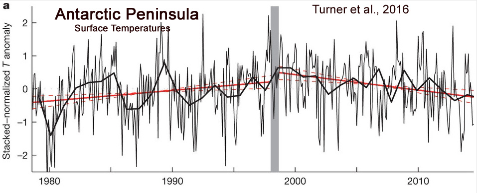
Turner et al., 2016 Absence of 21st century warming on Antarctic Peninsula consistent with natural variability … Since the 1950s, research stations on the Antarctic Peninsula have recorded some of the largest increases in near-surface air temperature in the Southern Hemisphere. This warming has contributed to the regional retreat of glaciers, disintegration of floating ice shelves and a ‘greening’ through the expansion in range of various flora. Several interlinked processes have been suggested as contributing to the warming, including stratospheric ozone depletion, local sea-ice loss, an increase in westerly winds, and changes in the strength and location of low–high-latitude atmospheric teleconnections. Here we use a stacked temperature record to show an absence of regional [Antarctic Peninsula] warming since the late 1990s. The annual mean temperature has decreased at a statistically significant rate, with the most rapid cooling during the Austral summer.
Previdi and Polvani, 2016 Global and regional climate models robustly simulate increases in Antarctic surface mass balance (SMB) during the twentieth and twenty-first centuries in response to anthropogenic global warming. Despite these robust model projections, however, observations indicate that there has been no significant change in Antarctic SMB [surface mass balance] in recent decades. We show that this apparent discrepancy between models and observations can be explained by the fact that the anthropogenic climate change signal during the second half of the twentieth century is small compared to the noise associated with natural climate variability. Using an ensemble of 35 global coupled climate models to separate signal and noise, we find that the forced SMB increase due to global warming in recent decades is unlikely to be detectable as a result of large natural SMB variability. However, our analysis reveals that the anthropogenic impact on Antarctic SMB is very likely to emerge from natural variability by the middle of the current century, thus mitigating future increases in global sea level.
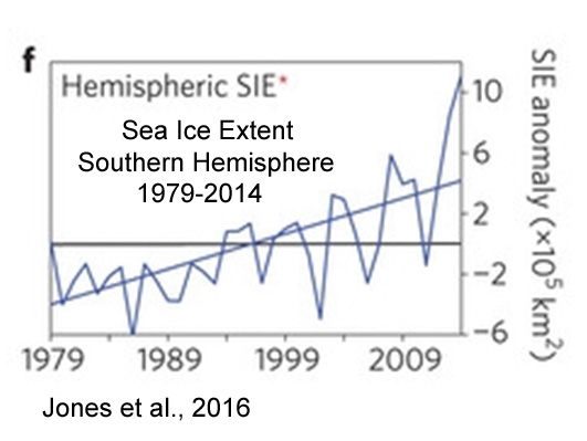
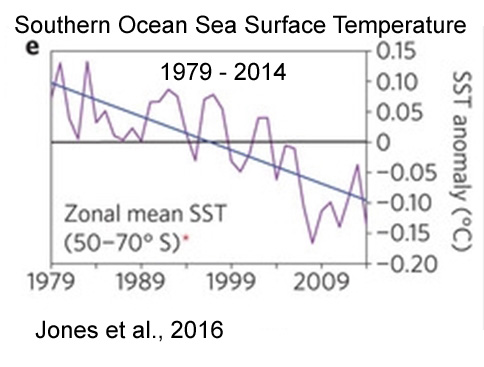
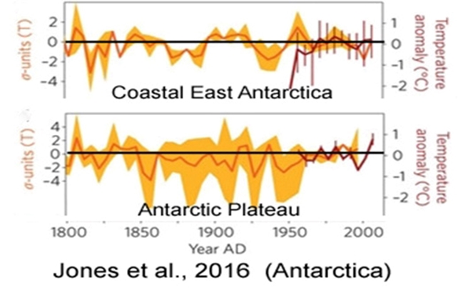
Jones et al., 2016 Understanding the causes of recent climatic trends and variability in the high-latitude Southern Hemisphere is hampered by a short instrumental record. Here, we analyse recent atmosphere, surface ocean and sea-ice observations in this region and assess their trends in the context of palaeoclimate records and climate model simulations. Over the 36-year satellite era, significant linear trends in annual mean sea-ice extent, surface temperature and sea-level pressure are superimposed on large interannual to decadal variability. Most observed trends, however, are not unusual when compared with Antarctic palaeoclimate records of the past two centuries. With the exception of the positive trend in the Southern Annular Mode, climate model simulations that include anthropogenic forcing are not compatible with the observed trends. This suggests that natural variability overwhelms the forced response in the observations, but the models may not fully represent this natural variability or may overestimate the magnitude of the forced response.
Cook et al., 2016 In recent decades, hundreds of glaciers draining the Antarctic Peninsula (63° to 70°S) have undergone systematic and progressive change. These changes are widely attributed to rapid increases in regional surface air temperature, but it is now clear that this cannot be the sole driver. Here, we identify a strong correspondence between mid-depth ocean temperatures and glacier-front changes along the ~1000-kilometer western coastline. In the south, glaciers that terminate in warm Circumpolar Deep Water have undergone considerable retreat, whereas those in the far northwest, which terminate in cooler waters, have not. Furthermore, a mid-ocean warming since the 1990s in the south is coincident with widespread acceleration of glacier retreat. We conclude that changes in ocean-induced melting are the primary cause of retreat for glaciers in this region. [S]everal recent studies of Arctic glaciers have concluded that calving rates are strongly dependent on ocean temperatures. Until now, the role of the ocean (as opposed to the atmosphere) as the dominant driver of glacier frontal retreat on the western AP has not been considered…. We conclude that ocean temperatures below 100-m depth have been the predominant control on multidecadal glacier front behavior in the western AP.
Ekaykin et al., 2016 We then compared recent temperature variability in the PEL region with indices of Southern Hemisphere modes of variability, and highlight the importance of the Annular Antarctic Oscillation and the Interdecadal Pacific Oscillation that in total explain 59% of the temperature variance in this Antarctic region. At the multi-decadal time-scale, however, temperature variations appear most closely related with the Indian Ocean Dipole mode, understood to modulate the cyclonic activity bringing heat and moisture to Princess Elisabeth Land (East Antarctica).
Gooch et al., 2016 We present the results of two numerical models describing contributions of groundwater and heterogeneous heat sources to ice dynamics directly relevant to basal processes in East Antarctica. A two-phase, one-dimensional hydrothermal model demonstrates the importance of groundwater flow in vertical heat flux advection near the ice-bed interface. Typical, conservative vertical components of groundwater volume fluxes (from either topographical gradients or vertically channeled flow) on the order of ±1–10 mm/yr can alter vertical heat flux by ±50–500 mW/m2 given parameters typical for the interior of East Antarctica. This heat flux has the potential to produce considerable volumes of meltwater depending on basin geometry and geothermal heat production. A one-dimensional hydromechanical model demonstrates that groundwater is mainly recharged into saturated, partially poroelastic (i.e., vertical stress only; not coupled to a deformation equation) sedimentary aquifers during ice advance. During ice retreat, groundwater discharges into the ice-bed interface, which may contribute to water budgets on the order of 0.1–1 mm/yr.
Comiso et al., 2016 The Antarctic sea ice extent has been slowly increasing contrary to expected trends due to global warming and results from coupled climate models. After a record high extent in 2012 the extent was even higher in 2014 when the magnitude exceeded 20×106 km2 for the first time during the satellite era. … [T]he [increasing] trend in sea ice cover is strongly influenced by the [decreasing] trend in surface temperature. … With a few exceptions, the regions where the trends in the sea ice cover are observed to be positive as depicted in Fig. 6 are also the general location where the temperature trends are negative indicating a general cooling as would be expected. For example, the regions near 0°E and 170°E where strong positive trend in sea ice have been observed are also the regions where strong negative trends in surface temperatures are observed.
Pauling et al., 2016 The possibility that recent Antarctic sea ice expansion resulted from an increase in freshwater reaching the Southern Ocean is investigated here. … Two sets of experiments were conducted from 1980 to 2013 in CESM1(CAM5), one of the CMIP5 models, artificially distributing freshwater either at the ocean surface to mimic iceberg melt or at the ice shelf fronts at depth. An anomalous reduction in vertical advection of heat into the surface mixed layer resulted in sea surface cooling at high southern latitudes and an associated increase in sea ice area. Enhancing the freshwater input by an amount within the range of estimates of the Antarctic mass imbalance did not have any significant effect on either sea ice area magnitude or trend. Freshwater enhancement of raised the total sea ice area by 1 × 10⁶ km2, yet this and even an enhancement of was insufficient to offset the sea ice decline due to anthropogenic forcing for any period of 20 years or longer. Further, the sea ice response was found to be insensitive to the depth of freshwater injection.
Kwok et al., 2016 Previous work have shown that sea ice variability in the south Pacific is associated with extra-tropical atmospheric anomalies linked to the Southern Oscillation (SO). Over a 32-year period (1982-2013), our study shows that the trend in Southern Oscillation index (SOI) is also able to quantitatively explain the trends in sea-ice edge, drift, and surface winds in this region. On average two-thirds of the winter ice-edge trend in this sector, linked to ice drift and surface winds, could be explained by the positive SOI trend thus subjecting the ice edge to strong decadal SO variability. If this relationship holds, the negative SOI trend prior to the recent satellite era suggests ice edge trends opposite to that of the recent record over a similar time scale. Significant low frequency ice edge trends, linked to the natural variability of SO, are superimposed upon any trends expected of anthropogenic forcing.
Hobbs et al., 2016 Observations show that Southern Ocean sea ice extent has increased since 1979, whereas global coupled climate models simulate a decrease over the same period. It is uncertain whether the observed trends are anthropogenically forced or due to internal variability, and whether the discrepancy between models and observations is also due to internal variability or indicative of a significant deficiency in the models. ….The Ross Sea is a confounding factor, with a significant increase in sea ice since 1979 that is not captured by climate models; however, existing proxy reconstructions of this region are not yet sufficiently reliable for formal change detection.
Purich et al., 2016 Despite global warming, total Antarctic sea ice coverage increased over 1979–2013. However, the majority of Coupled Model Intercomparison Project phase 5 models simulate a decline. Mechanisms causing this discrepancy have so far remained elusive. Here we show that weaker trends in the intensification of the Southern Hemisphere westerly wind jet simulated by the models may contribute to this disparity. During austral summer, a strengthened jet leads to increased upwelling of cooler subsurface water and strengthened equatorward transport, conducive to increased sea ice. As the majority of models underestimate summer jet trends, this cooling process is underestimated compared with observations and is insufficient to offset warming in the models. Through the sea ice-albedo feedback, models produce a high-latitude surface ocean warming and sea ice decline, contrasting the observed net [surface ocean] cooling and sea ice increase. A realistic simulation of observed wind changes may be crucial for reproducing the recent observed sea ice increase.
Sobota et al., 2016 This study investigated the surge dynamics of Aavatsmarkbreen, a glacier in Svalbard and its geomorphological impact based on remote sensing data and field observations. The main objective was to analyse and classify subglacial and supraglacial landforms in the context of glacial deformation and basal sliding over a thin layer of thawed, water-saturated deposits. The study also focused on the geomorphological evidence of surge-related sub- and supraglacial crevassing and glacier front fracturing. From 2006 to 2013, the average recession of Aavatsmarkbreen was 363 m (52 m a−1). A subsequent surge during 2013–2015 resulted in a substantial advance of the glacier front of over 1 km and an increase in its surface area of more than 2 km2.
Jahn et al., 2016 Climate model simulations give a large range of over 100 years for predictions of when the Arctic could first become ice free in the summer, and many studies have attempted to narrow this uncertainty range. However, given the chaotic nature of the climate system, what amount of spread in the prediction of an ice-free summer Arctic is inevitable? Based on results from large ensemble simulations with the Community Earth System Model, we show that internal variability alone leads to a prediction uncertainty of about two decades, while scenario uncertainty between the strong (Representative Concentration Pathway (RCP) 8.5) and medium (RCP4.5) forcing scenarios adds at least another 5 years. Common metrics of the past and present mean sea ice state (such as ice extent, volume, and thickness) as well as global mean temperatures do not allow a reduction of the prediction uncertainty from internal variability.
Toyota et al., 2016 In late winter-early spring 2012, the second Sea Ice Physics and Ecosystems Experiment (SIPEX II) was conducted off Wilkes Land, East Antarctica, onboard R/V Aurora Australis. The sea-ice conditions were characterized by significantly thick first-year ice and snow, trapping the ship for about 10 days in the near coastal region. The deep snow cover was particularly remarkable, in that its average value of 0.45 m was almost three times that observed between 1992 and 2007 in the region. … Based on these results, we deduce that lower loss of snow into leads was probably responsible for the extraordinary snow in 2012. Statistical analysis and satellite images suggest that the reduction in loss of snow into leads is attributed to rough ice surface associated with active deformation processes and larger floe size due to sea-ice expansion. This highlights the importance of snow-sea ice interaction in determining the mean snow depth on Antarctic sea ice.
Meehl et al., 2016 Antarctic sea-ice extent has been slowly increasing in the satellite record that began in 1979. Since the late 1990s, the increase has accelerated, but the average of all climate models shows a decline. Meanwhile, the Interdecadal Pacific Oscillation, an internally generated mode of climate variability, transitioned from positive to negative, with an average cooling of tropical Pacific sea surface temperatures, a slowdown of the global warming trend, and a deepening of the Amundsen Sea Low near Antarctica that has contributed to regional circulation changes in the Ross Sea region and expansion of sea ice. Here we show that the negative phase of the Interdecadal Pacific Oscillation in global coupled climate models is characterized by anomalies similar to the observed sea-level pressure and near-surface 850 hPa wind changes near Antarctica since 2000 that are conducive to expanding Antarctic sea-ice extent, particularly in the Ross Sea region in all seasons, involving a deepening of the Amundsen Sea Low. These atmospheric circulation changes are shown to be mainly driven by precipitation and convective heating anomalies related to the Interdecadal Pacific Oscillation in the equatorial eastern Pacific, with additional contributions from convective heating anomalies in the South Pacific convergence zone and tropical Atlantic regions.
Wang et al., 2016 “Pamir–Karakoram–Western-Kunlun-Mountain (northwestern Tibetan Plateau) Glacier Anomaly” has been a topic of debate due to the balanced, or even slightly positive glacier mass budgets in the early 21st century. Here we focus on the evolution of glaciers on the western Kunlun Mountain and its comparison with those from other regions of the Tibetan Plateau. The possible driver for the glacier evolution is also discussed. Western Kunlun Mountain glaciers reduce in area by 0.12 % yr−1 from 1970s to 2007–2011. However, there is no significant area change after 1999. Averaged glacier thickness loss is 0.08 ± 0.09 m yr−1 from 1970s to 2000, which is in accordance with elevation change during the period 2003–2008 estimated by the ICESat laser altimetry measurements. These further confirm the anomaly of glaciers in this region. Slight glacier reduction over the northwestern Tibetan Plateau may result from more accumulation from increased precipitation in winter which to great extent protects it from mass reductions under climate warming during 1961–2000. Warming slowdown since 2000 happening at this region may further mitigate glacier mass reduction, especially for the early 21st century.
Singh et al., 2016 We use a global climate model to study the effect of flattening the orography of the Antarctic Ice Sheet on climate. A general result is that the Antarctic continent and the atmosphere aloft warm, while there is modest cooling globally. The large local warming over Antarctica leads to increased outgoing longwave radiation, which drives anomalous southward energy transport towards the continent and cooling elsewhere. Atmosphere and ocean both anomalously transport energy southward in the Southern Hemisphere. Near Antarctica, poleward energy and momentum transport by baroclinic eddies strengthens. Anomalous southward cross-equatorial energy transport is associated with a northward shift of the inter-tropical convergence zone. In the ocean, anomalous southward energy transport arises from a slowdown of the upper cell of the oceanic meridional overturning circulation and a weakening of the horizontal ocean gyres, causing sea ice in the Northern Hemisphere to expand and the Arctic to cool. Comparison with a slab ocean simulation confirms the importance of ocean dynamics in determining the climate system response to Antarctic orography. We conclude by briefly discussing the relevance of these results to climates of the past and to future climate scenarios.
Nakamura et al., 2016 The results confirm a crucial role of the stratosphere in the sea-ice impacts on the mid-latitudes by coupling between the stratospheric polar vortex and planetary-scale waves. Those results and consistency with observation-based evidence suggest that a recent Arctic sea-ice loss is linked to mid-latitudes extreme weather events associated with the negative AO [Arctic Oscillation] phase.
Koutnik et al., 2016 The West Antarctic Ice Sheet Divide Core (WDC) provided a high-resolution climate record from near the Ross-Amundsen Divide in Central West Antarctica. In addition, radar-detected internal layers in the vicinity of the WDC site have been dated directly from the ice core to provide spatial variations in the age structure of the region. … Results show that the centennially averaged accumulation rate was over 20% lower than modern at 9.2 kyr before present (B.P.), increased by 40% from 9.2 to 2.3 kyr B.P., and decreased by at least 10% over the past 2 kyr B.P. to the modern values; these Holocene accumulation-rate changes in Central West Antarctica are larger than changes inferred from East Antarctic ice-core records. Despite significant changes in accumulation rate, throughout the Holocene the regional accumulation pattern has likely remained similar to today, and the ice-divide position has likely remained on average within 5 km of its modern position. Continent-scale ice-sheet models used for reconstructions of West Antarctic ice volume should incorporate this accumulation history.
Purich et al., 2016 A strengthening of the Amundsen Sea Low from 1979-2013 has been shown to largely explain the observed increase in Antarctic sea ice concentration in the eastern Ross Sea and decrease in the Bellingshausen Sea. Here we show that while these changes are not generally seen in freely-running coupled climate model simulations, they are reproduced in simulations of two independent coupled climate models; one constrained by observed sea surface temperature anomalies in the tropical Pacific, and the other by observed surface wind-stress in the tropics. Our analysis confirms previous results and strengthens the conclusion that the phase change in the Interdecadal Pacific Oscillation from positive to negative over 1979-2013 contributed to the observed strengthening of the Amundsen Sea Low and associated pattern of Antarctic sea ice change during this period. New support for this conclusion is provided by simulated trends in spatial patterns of sea ice concentrations that are similar to those observed. Our results highlight the importance of accounting for teleconnections from low to high latitudes in both model simulations and observations of Antarctic sea ice variability and change.
Andres, 2016 Most of the historical Greenland climate reconstructions are restricted to the industrial period, due to a lack of spatially-comprehensive climate records. They exhibit substantial differences in the timing, phasing and amplitudes of past climate variations, due to regional sensitivities in the source data and the reconstruction methodologies. Reconstructions indicate that Greenland temperatures did not begin to follow hemispheric greenhouse gas warming patterns until the mid-1990s. This discrepancy indicates either that the warming hiatus was associated with internal climate variability, or that the simulations are missing processes important to Greenland climate. For example, indirect effects of anthropogenic aerosols are not captured in the climate model employed here.
Colucci, 2016 The evolution of glaciers and ice patches, as well as the equilibrium-line altitude (ELA) since the Little Ice Age (LIA) maximum were investigated in the Julian Alps (south-eastern European Alps) including ice masses that were previously unreported. … The ELAs of the two major LIA glaciers (Canin and Triglav) have been established at 2275 ± 10 m and 2486 ± 10 m, respectively, by considering the reconstructed area and digital elevation model (DEM) and using an accumulation area ratio (AAR) of 0.44 ± 0.07, typical of small cirque glaciers. Changes in the ELA and glaciers extension indicate a decoupling from climate. This is most evident in the smallest avalanche-dominated ice bodies, which are currently controlled mainly by precipitation. The damming effect of moraine ridges and pronival ramparts at the snout of small ice bodies in the Julian Alps represents a further geomorphological control on the evolution of such ice masses, which seem to be resilient to recent climate warming instead of rapidly disappearing as should be expected
Lenaerts et al., 2016 We present climate and surface mass balance (SMB) of the Antarctic ice sheet (AIS) as simulated by the global, coupled ocean–atmosphere–land Community Earth System Model (CESM) with a horizontal resolution of ∼1∘ in the past, present and future (1850–2100). CESM correctly simulates present-day Antarctic sea ice extent, large-scale atmospheric circulation and near-surface climate, but fails to simulate the recent expansion of Antarctic sea ice. The present-day Antarctic ice sheet SMB equals 2280±131 Gtyear−1, which concurs with existing independent estimates of AIS SMB. When forced by two CMIP5 climate change scenarios (high mitigation scenario RCP2.6 and high-emission scenario RCP8.5), CESM projects an increase of Antarctic ice sheet SMB of about 70 Gtyear−1 per degree warming. This increase is driven by enhanced snowfall, which is partially counteracted by more surface melt and runoff along the ice sheet’s edges. This intensifying hydrological cycle is predominantly driven by atmospheric warming, which increases (1) the moisture-carrying capacity of the atmosphere, (2) oceanic source region evaporation, and (3) summer AIS cloud liquid water content.
Armour et al., 2016 The Southern Ocean has shown little warming over recent decades, in stark contrast to the rapid warming observed in the Arctic. Along the northern flank of the Antarctic Circumpolar Current, however, the upper ocean has warmed substantially. Here we present analyses of oceanographic observations and general circulation model simulations showing that these patterns—of delayed warming south of the Antarctic Circumpolar Current and enhanced warming to the north—are fundamentally shaped by the Southern Ocean’s meridional overturning circulation: wind-driven upwelling of unmodified water from depth damps warming around Antarctica; greenhouse gas-induced surface heat uptake is largely balanced by anomalous northward heat transport associated with the equatorward flow of surface waters; and heat is preferentially stored where surface waters are subducted to the north. Further, these processes are primarily due to passive advection of the anomalous warming signal by climatological ocean currents; changes in ocean circulation are secondary. These findings suggest the Southern Ocean responds to greenhouse gas forcing on the centennial, or longer, timescale over which the deep ocean waters that are upwelled to the surface are warmed themselves. It is against this background of gradual warming that multidecadal Southern Ocean temperature trends must be understood.
Fausto et al., 2016 During two exceptionally large July 2012 multiday Greenland ice sheet melt episodes, nonradiative energy fluxes (sensible, latent, rain, and subsurface collectively) dominated the ablation area surface energy budget of the southern and western ice sheet. On average the nonradiative energy fluxes contributed up to 76% of daily melt energy at nine automatic weather station sites in Greenland. Comprising 6% of the ablation period, these powerful melt episodes resulted in 12–15% of the south and west Greenland automatic weather station annual ablation totals. Analysis of high resolution (~5 km) HIRHAM5 regional climate model output indicates widespread dominance of nonradiative energy fluxes across the western ablation area during these episodes. Yet HIRHAM5 still underestimates melt by up to 56% during these episodes due to a systematic underestimation of turbulent energy fluxes typical of regional climate models. This has implications for underestimating future melt, when exceptional melt episodes are expected to occur more frequently.
Jamieson et al., 2016 The subglacial landscape of Princess Elizabeth Land (PEL) in East Antarctica is poorly known due to a paucity of ice thickness measurements. This is problematic given its importance for understanding ice sheet dynamics and landscape and climate evolution. To address this issue, we describe the topography beneath the ice sheet by assuming that ice surface expressions in satellite imagery relate to large-scale subglacial features. We find evidence that a large, previously undiscovered subglacial drainage network is hidden beneath the ice sheet in PEL. We interpret a discrete feature that is 140 × 20 km in plan form, and multiple narrow sinuous features that extend over a distance of ∼1100 km. We hypothesize that these are tectonically controlled and relate to a large subglacial basin containing a deep-water lake in the interior of PEL linked to a series of long, deep canyons. The presence of 1-km-deep canyons is confirmed at a few localities by radio-echo sounding data, and drainage analysis suggests that these canyons will direct subglacial meltwater to the coast between the Vestfold Hills and the West Ice Shelf.
Pattyn et al., 2016 Subglacial lakes have long been considered hydraulically isolated water bodies underneath ice sheets. This view changed radically with the advent of repeat-pass satellite altimetry and the discovery of multiple lake discharges and water infill, associated with water transfer over distances of more than 200 km. The presence of subglacial lakes also influences ice dynamics, leading to glacier acceleration. Furthermore, subglacial melting under the Antarctic ice sheet is more widespread than previously thought, and subglacial melt rates may explain the availability for water storage in subglacial lakes and water transport.
Zhang et al., 2016 The assessment of glacier mass budget is crucial for assessing water reserves stored in glaciers. Derived glacier mass changes in the Muztag Ata and Kongur Tagh (MAKT) region in the eastern Pamir, northwestern China, is helpful in improving our knowledge of the dynamics of glaciers under a changing climate in High Mountain Asia. Here, glacier area and mass changes derived from remote sensing data are investigated for the period 1971/76–2013/14 for glaciers in MAKT. We have used ASTER images (2013/14), Cartosat-1 (2014) and Landsat, SRTM (Shuttle Radar Terrain Mission) digital elevation model (DEM) (2000), topographic maps (1971/76) and the first and second Chinese glacier inventories (CGIs). Our results indicated that the glacier area of MAKT decreased from 1018.3 ± 12.99 km2 in 1971/ 76 to 999.2 ± 31.22 km2 in 2014 (–1.9 ± 0.2%). Weak area shrinkage of glaciers by 2.5 ± 0.5 km2 (0.2 ± 0.1%) happened after 2000 and the period 2009–2014 even saw a slight expansion by 0.5 ± 0.1 km2 (0.1 ± 0.0%). The glaciers in this region have experienced an overall loss of –6.99 ± 0.80 km3 in ice volume or –0.15 ± 0.12 m water equivalent (w.e.) a–1 from 1971/76 to 2013/14. The mass budget of MAKT was –0.19 ± 0.19 m w.e. a−1 for the period ~1971/76–1999 and –0.14 ± 0.24 m w.e. a−1 during 1999–2013/2014. Similar to previous studies, there has been little mass change in the Pamir over recent decades despite such uncertainties. Glacier mass change showed spatial and temporal heterogeneity, with strong mass loss on debris-covered glaciers with an average of –0.32 ± 0.12 m w.e. a−1 from the 1970s to 2013/14.
VI. Ocean Acidification? (14)
Doblin and van Sebille, 2016 Here we show that upper-ocean microbes experience along-trajectory temperature variability up to 10 °C greater than seasonal fluctuations estimated in a static frame, and that this variability depends strongly on location. These findings demonstrate that drift in ocean currents can increase the thermal exposure of microbes and suggests that microbial populations with broad thermal tolerance will survive transport to distant regions of the ocean and invade new habitats.
(press release) The results of the study … show for the first time the range of temperatures that plankton travel through. In most locations, they endure temperature extremes that go beyond what is predicted by models of global warming.
Moore, 2016 If the forecasts of continued global warming are borne out, the oceans will also become warmer and will tend to outgas CO2, offsetting to some extent the small increased partial pressure that might otherwise occur. … An analysis of research on the effect of lower pH shows a net beneficial impact on the calcification, metabolism, growth, fertility, and survival of calcifying marine species when pH is lowered up to 0.3 units, which is beyond what is considered a plausible reduction during this century. … There is no evidence to support the claim that most calcifying marine species will become extinct owing to higher levels of CO2 in the atmosphere and lower pH in the oceans.
Schram et al., 2016 The present study investigated the effects of elevated seawater temperature and decreased pH on growth (wet mass and shell morphometrics), net calcification, and proximate body composition (protein and lipid) of body tissues in two common benthic gastropods. .. Following a 6-week exposure, limpets showed no temperature or pH effects on whole body mass or net calcification. Despite no significant differences in whole body mass, the shell length and width of limpets at elevated temperature tended to grow less than those at ambient temperature. There was a significant interaction between the sex of limpets and pH. There were no significant temperature or pH effects on growth, net calcification, shell morphologies, or proximate body composition of snails. Our findings suggest that both gastropod species demonstrate resilience to initial exposure to temperature and pH changes predicted to occur over the next several hundred years globally and perhaps sooner along the WAP.
Uthicke et al., 2016 Near the vent site, the urchins experienced large daily variations in pH (> 1 unit) andpCO2 (> 2000 ppm) and average pH values (pHT 7.73) much below those expected under the most pessimistic future emission scenarios. Growth was measured over a 17-month period using tetracycline tagging of the calcareous feeding lanterns. Average-sized urchins grew more than twice as fast at the vent compared with those at an adjacent control site, and assumed larger sizes at the vent compared to the control site and two other sites at another reef near-by. … Thus, urchins did not only persist but actually ‘thrived’ under extreme CO2 conditions.
Prada et al., 2016 Our study suggests that populations of Orbicella species [corals] are capable of rebounding from reductions in population size under suitable conditions and that the effective population size of modern corals provides rich standing genetic variation for corals to adapt to climate change.
Brien et al., 2016 Corals were collected from reefs around Orpheus and Pelorus Islands on the Great Barrier Reef, Australia. They were then exposed to elevated pCO2 for 4 weeks with two CO2treatments: intermediate (pCO2 648) and high (pCO2 1003) compared with a control (unmanipulated seawater) treatment (pCO2 358). Porites cylindrica growth did not vary among pCO2 treatments, regardless of the presence and type of competitors, nor was the growth of another hard coral species, Acropora cerealis, affected by pCO2 treatment.
McGowan et al., 2016 Quantification of CO2 exchange with the atmosphere over coral reefs has relied on micro-scale measurements of pCO2 gradients across the air-sea interfacial boundary; shipboard measurements of air-sea CO2 exchange over adjacent ocean inferred to represent over reef processes, or ecosystem productivity modelling. Here we present by way of case study the first direct measurements of air-sea CO2 exchange over a coral reef made using the eddy covariance method. Research was conducted during the summer monsoon over a lagoonal platform reef in the southern Great Barrier Reef, Australia. Results show the reef flat to be a net source of CO2 to the atmosphere of similar magnitude as coastal lakes, while adjacent shallow and deep lagoons were net sinks as was the surrounding ocean. This heterogeneity in CO2 exchange with the atmosphere confirms need for spatially representative direct measurements of CO2 over coral reefs to accurately quantify their role in atmospheric carbon budgets.
Zhang et al., 2016 The present study investigated the physiological responses (ingestion, absorption rate and efficiency, respiration, and excretion) and scope for growth (SfG) of an intertidal scavenging gastropod, Nassarius festivus, to the combined effects of ocean acidification (pCO2 levels: 380, 950, and 1250 µatm), salinity (10 and 30 psu), and temperature (15 and 30°C) for 31 d. Low salinity (10 psu) reduced ingestion, absorption rate, respiration, excretion, and SfG of N. festivus throughout the exposure period. Low temperature (15°C) had a similar effect on these parameters, except for SfG at the end of the exposure period (31 d). However, elevated pCO2 levels had no effects in isolation on all physiological parameters and only weak interactions with temperature and/or salinity for excretion and SfG. In conclusion, elevatedpCO2 will not affect the energy budget of adult N. festivus at the pCO2level predicted to occur by the Intergovernmental Panel on Climate Change (IPCC) in the year 2300.
Hildebrandt et al., 2016 It is currently under debate whether organisms that regulate their acid–base status under environmental hypercapnia demand additional energy. … During the SOPRAN mesocosm experiment in Bergen, Norway, 2011, we weekly collected Calanus finmarchicus from mesocosms initially adjusted to 390 and 3000 µatm CO2 and measured grazing at low and high pCO2. In addition, copepods were deep frozen for body mass analyses. Elevated pCO2 did not directly affect grazing activities and body mass, suggesting that the copepods did not have additional energy demands for coping with acidification, neither during long-term exposure nor after immediate changes in pCO2. Shifts in seawater pH thus do not seem to challenge these copepod species.
Cross et al., 2016 A CO2 perturbation experiment was performed on the New Zealand terebratulide brachiopod Calloria inconspicua to investigate the effects of pH conditions predicted for 2050 and 2100 on the growth rate and ability to repair shell. Three treatments were used: an ambient pH control (pH 8.16), a mid-century scenario (pH 7.79), and an end-century scenario (pH 7.62). The ability to repair shell was not affected by acidified conditions with >80% of all damaged individuals at the start of the experiment completing shell repair after 12 weeks. Growth rates in undamaged individuals >3 mm in length were also not affected by lowered pH conditions, whereas undamaged individuals <3 mm grew faster at pH 7.62 than the control. The capability of C. inconspicua to continue shell production and repair under acidified conditions suggests that this species has a robust control over the calcification process, where suitable conditions at the site of calcification can be generated across a range of pH conditions.
Heinrich et al., 2016 In this study, we tested the effects of elevated CO2 on the foraging and shelter-seeking behaviours of the reef-dwelling epaulette shark, Hemiscyllium ocellatum. Juvenile sharks were exposed for 30 d to control CO2 (400 µatm) and two elevated CO2treatments (615 and 910 µatm), consistent with medium- and high-end projections for ocean pCO2 by 2100. Contrary to the effects observed in teleosts and in some other sharks, behaviour of the epaulette shark was unaffected by elevated CO2.
Sunjin and Jetfelt, 2016 [A]n increasing number of studies show tolerance of fish to increased levels of carbon dioxide. … We investigated the possible effects of CO2 on behavioural lateralization, swimming activity, and prey and predator olfactory preferences, all behaviours where disturbances have previously been reported in other fish species after exposure to elevated CO2. Interestingly, we failed to detect effects of carbon dioxide for most behaviours investigated, excluding predator olfactory cue avoidance, where control fish initially avoided predator cue while the high CO2 group was indifferent. The present study therefore shows behavioural tolerance to increased levels of carbon dioxide in the goldsinny wrasse. We also highlight that individual fish can show disturbance in specific behaviours while being apparently unaffected by elevated pCO2 in other behavioural tests.
Vicente et al., 2016 Our goal was to determine if spicule biomineralization was enhanced or repressed by ocean acidification and thermal stress by monitoring silica uptake rates during short-term (48 h) experiments and comparing biomineralized tissue ratios before and after a long-term (26 d) experiment. In the short-term experiment, we found that silica uptake rates were not impacted by high pCO2 (1050 µatm), warmer temperatures (27°C), or combined high pCO2 with warmer temperature (1119 µatm; 27°C) treatments. The long-term exposure experiments revealed no effect on survival or growth rates of M. grandis to high pCO2 (1198 µatm), warmer temperatures (25.6°C), or combined high pCO2 with warmer temperature (1225 µatm, 25.7°C) treatments, indicating that M. grandiswill continue to prosper under predicted increases in pCO2 and sea surface temperature.
Wang et al., 2016 The pMENs results were in line with the null hypothesis that elevated pCO2/pH does not affect biogeochemistry processes. The number of nodes within the pMENs and the connectivity of the bacterial communities were similar, despite increased pCO2 concentrations. Our results indicate that elevated pCO2did not significantly affect microbial community structure and succession in the Arctic Ocean, suggesting bacterioplankton community resilience to elevated pCO2.
VII. Natural Climate Catastrophes – Without CO2 Changes (4)
Akkerman, 2016 European Middle Ages were an extended period of fluctuating but mostly above-average warm temperatures that by the tenth century had melted the ice sheet of the Arctic Ocean and brought about Viking marine exploration of, and temporary settlement on the eastern shores of North America. Medieval warm climate was punctuated by two short, but extremely cold events. The first was the cold event of 535–6, possibly due to a volcanic catastrophe in the tropics that yielded extensive atmospheric dust veil, followed by a major crop failure through Europe, North Africa and the Middle East, and a subsequent terrifying pandemic of the years 541–2, the Plague of Justinian. The second cold event coincided with a prolonged series of major volcanic eruptions on the Southern Hemisphere during 1315–1322. Extensive crop failure during the years 1315–1317 had led, at the same time, to the Great Famine throughout much of Europe.
Moros et al., 2016 Centennial to millennial scale changes in the wider North Atlantic region were accompanied by variations in the West Greenland Current (WGC). During periods of relatively warm WGC, increased surface air temperature over western Greenland led to ice sheet retreat and significant meltwater flux. In contrast, during periods of cold WGC, atmospheric cooling resulted in glacier advances. … We also identify potential linkages between the palaeoceanography of the Disko Bugt region and key changes in the history of human occupation. Cooler oceanographic conditions at 3.5 ka BP support the view that the Saqqaq culture left Disko Bugt due to deteriorating climatic conditions. The cause of the disappearance of the Dorset culture is unclear, but the new data presented here indicate that it may be linked to a significant increase in meltwater flux, which caused cold and unstable coastal conditions at ca. 2 ka BP [2,000 years before present]. The subsequent settlement of the Norse occurred at the same time as climatic amelioration during the Medieval Climate Anomaly and their disappearance may be related to harsher conditions at the beginning of the Little Ice Age.
Anderson, 2016 New developments in the collection of palaeo-data over the past two decades have transformed our understanding of climate and environmental history in eastern Africa. This article utilises instrumental and proxy evidence of historical lake-level fluctuations from Baringo and Bogoria, along with other Rift Valley lakes, to document the timing and magnitude of hydroclimate variability at decadal to century time scales since 1750. … The results reveal strong evidence of a catastrophic drought in the early nineteenth century, the effects of which radically alters our historical understanding of the character of settlement, mobility and identity within the Baringo–Bogoria basin.
Camenisch et al., 2016 The 1430s: a cold period of extraordinary internal climate variability during the early Spörer Minimum with social and economic impacts in north-western and central Europe … New evidence from proxy archives, historical documentary sources and climate model simulations permit us to provide an interdisciplinary, systematic assessment of an exceptionally cold period in the 15th century. Our assessment includes the role of internal, unforced climate variability and external forcing in shaping extreme climatic conditions and the impacts on and responses of the medieval society in north-western and central Europe. … The strong seasonal cycle in temperature reduced food production and led to increasing food prices, a subsistence crisis and a famine in parts of Europe. Societies were not prepared to cope with failing markets and interrupted trade routes.
VIII. Recent Cooling In The North Atlantic (3)
Duchez et al., 2016 [C]old ocean temperatures were the most extreme in the modern record [since the 1950s] over much of the mid-high latitude North-East Atlantic
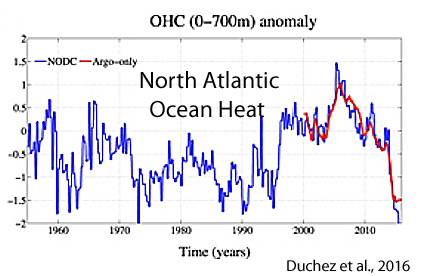
Robson et al., 2016 Here we show that since 2005 a large volume of the upper North Atlantic Ocean has cooled significantly by approximately 0.45 °C or 1.5 × 10²² J, reversing the previous warming trend. The observed cooling is not consistent with a dominant role for surface heat flux changes due to anthropogenic aerosols. Anthropogenic aerosol loads have decreased in the North Atlantic region since the 1990s, and would therefore be expected to have induced warming of Atlantic SSTs, in contrast to the observed cooling. The evidence we have presented is consistent with decadal variability in the NAO being a major driver of Atlantic Multidecadal Variability. .. . The decomposition of recent changes in deep Labrador Sea density into temperature and salinity contributions shows—perhaps surprisingly—that, although a deep ocean warming is dominating the low-density anomalies in the deep Labrador Sea since 1995, the waters here are not (yet) warmer than in the 1970s. … [Y]he magnitude of any anthropogenic contribution to this freshening is an open and important question. … [W]e would expect some further cooling of the North Atlantic to take place, in agreement with other studies. If the North Atlantic cools further this is likely to favour reduced rainfall in the Sahel region and drier summers in Northern Europe, as well as a continued suppression of hurricane numbers. Furthermore, the continuing cooling could have important implications for the Interdecadal Pacific Oscillation, and possibly global mean temperatures.
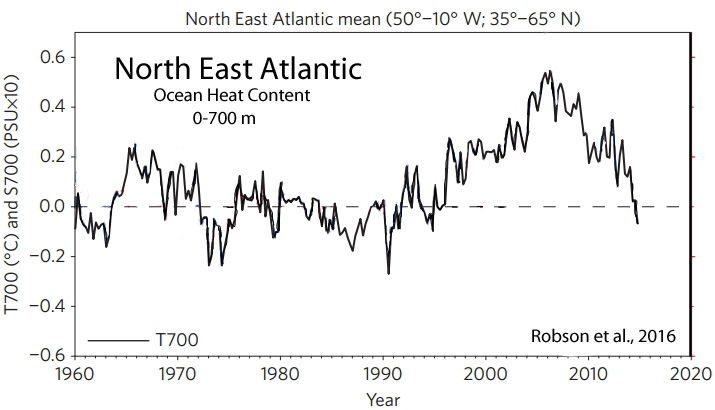
Chafik et al., 2016 The multidecadal variability of the North Atlantic Ocean has a strong signal in the sea surface temperature with many global climate linkages. An even stronger multidecadal signal can be found in the subpolar temperatures and salinities, where the Atlantic Water inflow variations constitute an essential part in the variability. The atmospheric forcing in the subpolar North Atlantic Ocean is dominated by the variability of the North Atlantic Oscillation (NAO), i.e., the leading mode of atmospheric variability in the North Atlantic sector, which modulates the atmosphere-ocean momentum and heat exchanges on a range of temporal scales. … These regime changes have recently been argued to be important for global mean surface temperature warming acceleration and hiatus.
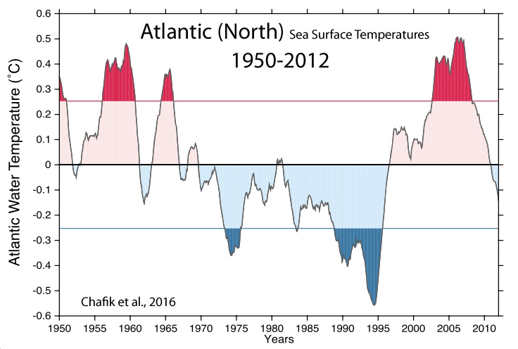


Recent Comments