Skeptic Papers 2018 (3)

3. Unsettled Science, Failed Climate Modeling (161)

Climate Model Unreliability/Biases/Errors (27)
Urban Heat Island: Raising Surface Temperatures Artificially (5)
Failing Renewable Energy, Climate Policies (18)
Wind Power Harming The Environment, Biosphere (19)
Elevated CO2: Greens Planet, Higher Crop Yields (20)
Polar Bear (and other) Populations Not Decreasing (10)
Global Warming Saves Lives. Cold Kills. (9)
Warming, Acidification Not Harming Oceanic Biosphere (11)
Coral Bleaching Is A Natural, Non-Anthropogenic Phenomenon (2)
No Increasing Trends In Intense Hurricanes/Storms (8)
No Increasing Trend In Drought/Flood Frequency, Severity (7)
Natural CO2 Emissions A Net Source, Not A Net Sink (5)
Global Fire Frequency Declining As CO2 Rises (2)
CO2 Changes Lag Temperature Changes By 1000+ Years (3)
Global Losses/Deaths From Weather Disasters Declining (2)
No AGW Changes To Hydrological Cycle Detectable (6)
Peak Oil As Myth (3)
Miscellaneous (16)

Climate Model Unreliability/Biases/Errors

Collins et al., 2018     Here there is a dynamical gap in our understanding. While we have conceptual models of how weather systems form and can predict their evolution over days to weeks, we do not have theories that can adequately explain the reasons for an extreme cold or warm, or wet or dry, winter at continental scales. More importantly, we do not have the ability to credibly predict such states. Likewise, we can build and run complex models of the Earth system, but we do not have adequate enough understanding of the processes and mechanisms to be able to quantitatively evaluate the predictions and projections they produce, or to understand why different models give different answers. … The global warming ‘hiatus’ provides an example of a climate event potentially related to inter-basin teleconnections. While decadal climate variations are expected, the magnitude of the recent event was unforeseen. A decadal period of intensified trade winds in the Pacific and cooler sea surface temperatures (SSTs) has been identified as a leading candidate mechanism for the global slowdown in warming.

Shen et al., 2018     The results showed that both future climate change (precipitation and temperature) and hydrological response predicted by the twenty GCMs [climate models] were highly uncertain, and the uncertainty increased significantly over time. For example, the change of mean annual precipitation increased from 1.4% in 2021–2050 to 6.5% in 2071–2100 for RCP4.5 in terms of the median value of multi-models, but the projected uncertainty reached 21.7% in 2021–2050 and 25.1% in 2071–2100 for RCP4.5.

Christy et al., 2018     [A]s new versions of the datasets are produced, trend magnitudes have changed markedly, for example the central estimate of the global trend of the mid-troposphere in Remote Sensing System’s increased 60% from +0.078 to +0.125°C decade−1, between consecutive versions 3.3 and 4.0 (Mears and Wentz 2016). … As an experiment, Mears et al. recalculated the RSS overall trend by simply truncating NOAA-14 data after 1999 (which reduced their long-term trend by 0.02 K decade⁻¹). However, this does not address the problem that the trends of the entire NOAA-12 and −14 time series (i.e. pre-2000) are likely too positive and thus still affect the entire time series. Additionally, the evidence from the Australian and U.S. VIZ comparisons support the hypothesis that RSS contains extra warming (due to NOAA-12, −14 warming.) Overall then, this analysis suggests spurious warming in the central estimate trend of RSS of at least +0.04°C decade⁻¹, which is consistent with results shown later based on other independent constructions for the tropical belt. … When examining all of the evidence presented here, i.e. the correlations, magnitude of errors and trend comparisons, the general conclusion is that UAH data tend to agree with (a) both unadjusted and adjusted IGRA radiosondes, (b) independently homogenized radiosonde datasets and (c) Reanalyses at a higher level, sometimes significantly so, than the other three [NOAA, RSS, UW]. … One key result here is that substantial evidence exists to show that the processed data from NOAA-12 and −14 (operating in the 1990s) were affected by spurious warming that impacted the four datasets, with UAH the least affected due to its unique merging process. RSS, NOAA and UW show considerably more warming in this period than UAH and more than the US VIZ and Australian radiosondes for the period in which the radiosonde instrumentation did not change. … [W]e estimate the global TMT trend is +0.10 ± 0.03°C decade−1. … The rate of observed warming since 1979 for the tropical atmospheric TMT layer, which we calculate also as +0.10 ± 0.03°C decade−1, is significantly less than the average of that generated by the IPCC AR5 climate model simulations. Because the model trends are on average highly significantly more positive and with a pattern in which their warmest feature appears in the latent-heat release region of the atmosphere, we would hypothesize that a misrepresentation of the basic model physics of the tropical hydrologic cycle (i.e. water vapour, precipitation physics and cloud feedbacks) is a likely candidate.

Abbott and Marohasy, 2018     While general circulation models are used by meteorological agencies around the world for rainfall forecasting, they do not generally perform well at forecasting medium-term rainfall, despite substantial efforts to enhance performance over many years. These are the same models used by the Intergovernmental Panel on Climate Change (IPCC) to forecast climate change over decades. Though recent studies suggest ANNs [artificial neural networks] have considerable application here, including to evaluate natural versus climate change over millennia, and also to better understand equilibrium climate sensitivity.

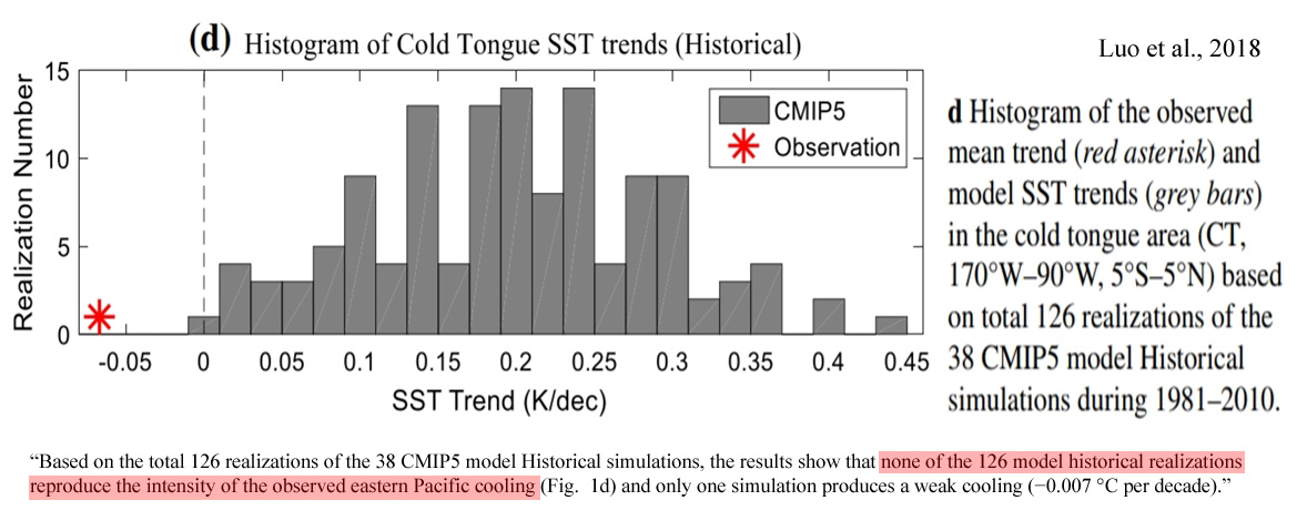
Luo et al., 2018     Over the recent three decades sea surface temperate (SST) in the eastern equatorial Pacific has decreased, which helps reduce the rate of global warming. However, most CMIP5 model simulations with historical radiative forcing do not reproduce this Pacific La Niña-like cooling. Based on the assumption of “perfect” models, previous studies have suggested that errors in simulated internal climate variations and/or external radiative forcing may cause the discrepancy between the multi-model simulations and the observation…. Based on the total 126 realizations of the 38 CMIP5 model Historical simulations, the results show that none of the 126 model historical realizations reproduce the intensity of the observed eastern Pacific cooling (Fig.  1d) and only one simulation produces a weak cooling (−0.007 °C per decade).

Ding et al., 2018     [W]e find that there was a warming hiatus/slowdown since 2005 at Ny-Ålesund. Additionally, the variation of air temperature lags by 8–9 years, which implies that the warming hiatus probably exists in the Arctic but lags behind, globally. This phenomenon is not an isolated instance, An et al. [2017] reported that the warming rate above 4000 m of the Tibetan Plateau has been slowing since the mid-2000s. In the Antarctic Peninsula, the slowdown of the increasing temperature trend was also found after 1998/1999, however, the reason is attributed to local phenomena, such as the deepening of Amundsen Sea Low and not due to the global hiatus [Turner et al., 2016]. … From the correlation analysis, we found Ny-Ålesund could represent most Arctic areas, especially the Atlantic-Arctic sector. … Especially air temperature, the record of Ny-Ålesund can capture the variation of surface temperature over most of [the] Arctic. … The oscillations of atmospheric dynamic systems, the methods of energy transport from low to high latitudes, and feedback mechanisms of the Arctic on climate change may contribute to the warming hiatus. … [C]limate changes in polar areas remain difficult to predict, which indicates that the underlying mechanisms of polar amplification remain uncertain and debatable.

Lacour et al., 2018     The representation of clouds over Greenland is a central concern for the models because clouds impact ice-sheet surface melt. We find that over Greenland, most of the models have insufficient cloud cover during summer. In addition, all models create too few non-opaque liquid containing clouds optically thin enough to let direct solar radiation reach the surface (-1% to -3.5% at the ground level). Some models create too few opaque clouds. In most climate models, the cloud properties biases identified over all Greenland also apply at Summit proving the value of the ground observatory in model evaluation. … At Summit, climate models underestimate cloud radiative effect (CRE) at the surface, especially in summer. The primary driver of the summer CRE biases compared to observations is the underestimation of the cloud cover in summer (-46% to -21%), which leads to an underestimated longwave radiative warming effect (CRELW = -35.7 W m-2 to -13.6 W m-2 compared to the ground observations) and an underestimated shortwave cooling effect (CRESW = +1.5 W m-2 to +10.5 W m-2 compared to the ground observations). Overall, the simulated [modeled] clouds do not radiatively warm the surface as much as observed. … Of particular importance, clouds can trigger surface melt over a large portion of the Greenland Ice Sheet (Bennartz et al. 2013; Solomon et al. 2017). Greenland surface melting increases non-linearly with increasing temperatures due to positive feedbacks between cloud microphysics, surface melting and surface albedo (Fettweis et al. 2013) and modulates the ice sheet mass balance (Van Tricht et al. 2016; Hofer et al. 2017). … Every model included in this study underestimates the net cloud radiative surface warming in summer. …  [O]nly few general circulation models are able to represent the surface of the Greenland ice sheet (Cullather et al. 2014). … Since the overall cloud radiative warming is underestimated in the models, we may expect an underestimate of Greenland surface melting. However, misrepresentation of clouds is not the only contributor to biases in the modeled surface melting.

Guo et al., 2018    The snow‐albedo feedback is a crucial component in high‐altitude cryospheric change but is poorly quantified over the Third Pole, encompassing the Karakoram and Tibetan Plateau. … [I]t is noteworthy that the magnitude of the constrained strength is only half of the unconstrained model estimate for the Third Pole, suggesting that current climate models generally overestimate the feedback of spring snow change to temperature change based on the unmitigated scenario.

Kravtsov et al., 2018     D]eviations of the model-simulated climate change from observations, such as a recent “pause” in global warming, have received considerable attention. Such decadal mismatches between model-simulated and observed climate trends are common throughout the twentieth century, and their causes are still poorly understood. While climate models exhibit various levels of decadal climate variability and some regional similarities to observations, none of the model simulations considered match the observed signal in terms of its magnitude, spatial patterns and their sequential time development. These results highlight a substantial degree of uncertainty in our interpretation of the observed climate change using current generation of climate models.

Essex and Tsonis, 2018     Climate models do not and cannot employ known physics fully. Thus, they are falsified, a priori.  Incomplete physics and the finite representation of computers can induce false instabilities. … [A[re there propositions that contemporary models make, crucial to their own objectives, that are falsifiable? Is there any physical test possible that would force us to conclude that they are unable to achieve their own objectives, thus requiring a rethinking of basic assumptions?  This paper addresses this question. But it is a question that cannot be comprehended in the face of many widely-held misconceptions about the direct meteorologically based projection modeling of climate. Foremost among these misconceptions is that climate models are full implementations of known, mature physics. This false conception can lead to the conclusion that falsification is irrelevant because models are simply an execution of previously known correct physics. … The empirical nature of large climate models can be clearly seen in their diverse outputs. If they followed the laws of physics in their entirety, they would all produce the same results under the same conditions. But they do not. In a recent study, the Climate Model Inter-comparison Project phase 3 (CMIP3) models [2] were considered and a detailed comparison at the dynamics level, using an approach involving climate networks [Steinhaeuser and Tsonis, 2013] was performed.  It was found that the models not only don’t agree with each other when it comes to dynamics, they also don’t agree with reality.

Kam et al., 2018     In summary, there is marginal evidence for an emerging detectable anthropogenic contribution toward earlier WSCT [winter-spring center time] in parts of North America. The regions with strongest relative indication of an anthropogenic contribution in our analysis include: the north-central U.S. (Region 3); the mountainous western U.S./southwestern Canada (Region 1); and extreme northeastern U.S. and Canadian Maritimes (Region 6). However, in none of the regions examined do a majority of the nine CMIP5 models examined robustly support a detectable attribution of an earlier (decreasing) WSCT trend to anthropogenic forcing. At some level, the difficulty in detecting a climate change signal comes down to low signal to noise ratio (Ziegler et al. 2005). Apparently, for the variable at hand, the climate change influence is not very large compared to interannual/interdecadal variability noise.

Bracegirdle et al., 2018     Our results show that the observed peak in multidecadal jet strength variability is even more unusual than NAO variability when compared to the model‐simulated range across 133 historical CMIP5 simulations. Some CMIP5 models appear capable of reproducing the observed low‐frequency peak in jet strength, but there are too few simulations of each model to clearly identify which.

Scafetta et al., 2018     The period from 2000 to 2016 shows a modest warming trend that the advocates of the anthropogenic global warming theory have labeled as the “pause” or “hiatus.” These labels were chosen to indicate that the observed temperature standstill period results from an unforced internal fluctuation of the climate (e.g. by heat uptake of the deep ocean) that the computer climate models are claimed to occasionally reproduce without contradicting the anthropogenic global warming theory (AGWT) paradigm. In part 1 of this work, it was shown that the statistical analysis rejects such labels with a 95% confidence because the standstill period has lasted more than the 15 year period limit provided by the AGWT advocates themselves. Anyhow, the strong warming peak observed in 2015-2016, the “hottest year on record,” gave the impression that the temperature standstill stopped in 2014. Herein, the authors show that such a temperature peak is unrelated to anthropogenic forcing: it simply emerged from the natural fast fluctuations of the climate associated to the El Niño-Southern Oscillation (ENSO) phenomenon. By removing the ENSO signature, the authors show that the temperature trend from 2000 to 2016 clearly diverges from the general circulation model (GCM) simulations. Thus, the GCMs models used to support the AGWT [anthropogenic global warming theory] are very likely flawed. By contrast, the semi-empirical climate models proposed in 2011 and 2013 by Scafetta, which are based on a specific set of natural climatic oscillations believed to be astronomically induced plus a significantly reduced anthropogenic contribution, agree far better with the latest observations.

Kundzewicz et al., 2018     Climate models need to be improved before they can be effectively used for adaptation planning and design. Substantial reduction of the uncertainty range would require improvement of our understanding of processes implemented in models and using finer resolution of GCMs and RCMs. However, important uncertainties are unlikely to be eliminated or substantially reduced in near future (cf. Buytaert et al., 2010). Uncertainty in estimation of climate sensitivity (change of global mean temperature, corresponding to doubling atmospheric CO2 concentration) has not decreased considerably over last decades. Higher resolution of climate input for impact models requires downscaling (statistical or dynamic) of GCM outputs, adding further uncertainty. … [C]limate models do not currently simulate the water cycle at sufficiently fine resolution for attribution of catchment-scale hydrological impacts to anthropogenic climate change. It is expected that climate models and impact models will become better integrated in the future. … Calibration and validation of a hydrological model should be done before applying it for climate change impact assessment, to reduce the uncertainty of results. Yet, typically, global hydrological models are not calibrated and validated. … Model-based projections of climate change impact on water resources can largely differ. If this is the case, water managers cannot have confidence in an individual scenario or projection for the future. Then, no robust, quantitative, information can be delivered and adaptation procedures need to be developed which use identified projection ranges and uncertainty estimates. Moreover, there are important, nonclimatic, factors affecting future water resources. … As noted by Funtowicz and Ravetz (1990), in the past, science was assumed to provide “hard” results in quantitative form, in contrast to “soft” determinants of politics, that were interest-driven and value-laden. Yet, the traditional assumption of the certainty of scientific information is now recognized as unrealistic and counterproductive. Policy-makers have to make “hard” decisions, choosing between conflicting options (with commitments and stakes being the primary focus), using “soft” scientific information that is bound with considerable uncertainty. Uncertainty has been policitized in that policy-makers have their own agendas that can include the manipulation of uncertainty. Parties in a policy debate may invoke uncertainty in their arguments selectively, for their own advantage.

Hanna et al., 2018     Recent changes in summer Greenland blocking captured by none of the CMIP5 models … Recent studies note a significant increase in high-pressure blocking over the Greenland region (Greenland Blocking Index, GBI) in summer since the 1990s. … We find that the recent summer GBI increase lies well outside the range of modeled past reconstructions (Historical scenario) and future GBI projections (RCP4.5 and RCP8.5). The models consistently project a future decrease in GBI (linked to an increase in NAO), which highlights a likely key deficiency of current climate models if the recently-observed circulation changes continue to persist. Given well-established connections between atmospheric pressure over the Greenland region and air temperature and precipitation extremes downstream, e.g. over Northwest Europe, this brings into question the accuracy of simulated North Atlantic jet stream changes and resulting climatological anomalies […] as well as of future projections of GrIS mass balance produced using global and regional climate models.

Lean, 2018     Climate change detection and attribution have proven unexpectedly challenging during the 21st century. Earth’s global surface temperature increased less rapidly from 2000 to 2015 than during the last half of the 20th century, even though greenhouse gas concentrations continued to increase. A probable explanation is the mitigation of anthropogenic warming by La Niña cooling and declining solar irradiance. Physical climate models overestimated recent global warming because they did not generate the observed phase of La Niña cooling and may also have underestimated cooling by declining solar irradiance. Ongoing scientific investigations continue to seek alternative explanations to account for the divergence of simulated and observed climate change in the early 21st century, which IPCC termed a “global warming hiatus.” … Understanding and communicating the causes of climate change in the next 20 years may be equally challenging. Predictions of the modulation of projected anthropogenic warming by natural processes have limited skill. The rapid warming at the end of 2015, for example, is not a resumption of anthropogenic warming but rather an amplification of ongoing warming by El Niño. Furthermore, emerging feedbacks and tipping points precipitated by, for example, melting summer Arctic sea ice may alter Earth’s global temperature in ways that even the most sophisticated physical climate models do not yet replicate.

Hunziker et al., 2018     About 40 % of the observations are inappropriate for the calculation of monthly temperature means and precipitation sums due to data quality issues. These quality problems undetected with the standard quality control approach strongly affect climatological analyses, since they reduce the correlation coefficients of station pairs, deteriorate the performance of data homogenization methods, increase the spread of individual station trends, and significantly bias regional temperature trends. Our findings indicate that undetected data quality issues are included in important and frequently used observational datasets and hence may affect a high number of climatological studies. It is of utmost importance to apply comprehensive and adequate data quality control approaches on manned weather station records in order to avoid biased results and large uncertainties.

Roach et al., 2018     Consistent biases in Antarctic sea ice concentration simulated by climate models … The simulation of Antarctic sea ice in global climate models often does not agree with observations. [M]odels simulate too much loose, low-concentration sea ice cover throughout the year, and too little compact, high-concentration cover in the summer. [C]urrent sea ice thermodynamics contribute to the inadequate simulation of the low-concentration regime in many models.

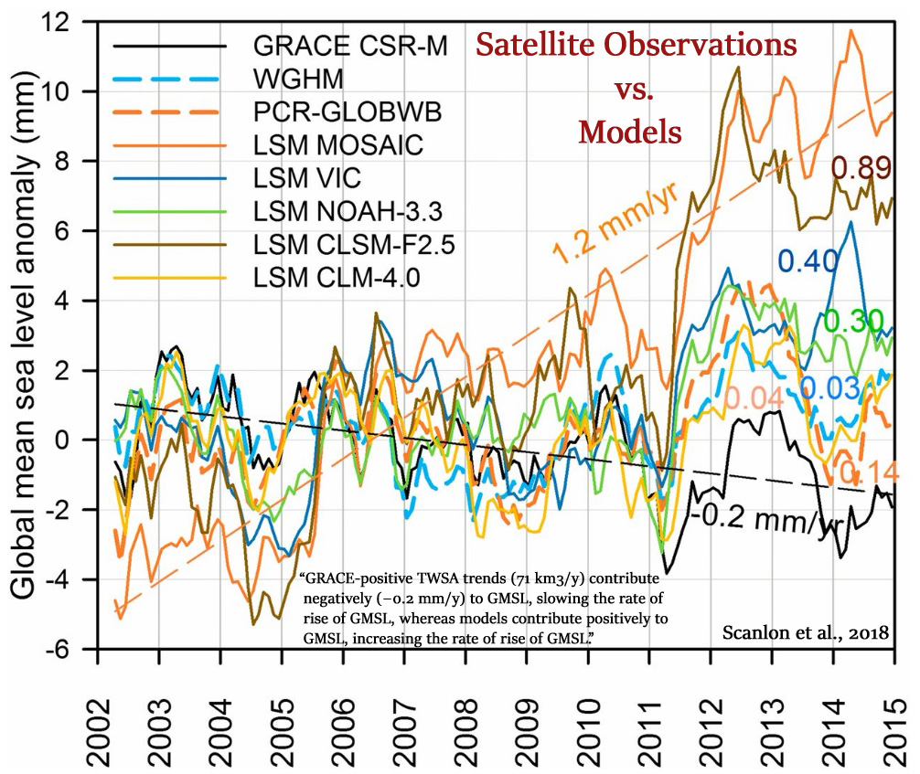
Scanlon et al., 2018     The models underestimate the large decadal (2002–2014) trends in water storage relative to GRACE satellites, both decreasing trends related to human intervention and climate and increasing trends related primarily to climate variations. The poor agreement between models and GRACE underscores the challenges remaining for global models to capture human or climate impacts on global water storage trends. … Increasing TWSA [total water storage anomalies] trends are found primarily in nonirrigated basins, mostly in humid regions, and may be related to climate variations. Models also underestimate median GRACE increasing trends (1.6–2.1 km³/y) by up to a factor of ∼8 in GHWRMs [global hydrological and water resource models] (0.3–0.6 km³/y). Underestimation of GRACE-derived TWSA increasing trends is much greater for LSMs [global land surface models], with four of the five LSMs [global land surface models] yielding opposite trends (i.e., median negative rather than positive trends) … Increasing GRACE trends are also found in surrounding basins, with most models yielding negative trends. Models greatly underestimate the increasing trends in Africa, particularly in southern Africa. .. TWSA trends from GRACE in northeast Asia are generally increasing, but many models show decreasing trends, particularly in the Yenisei. … Subtracting the modeled human intervention contribution from the total land water storage contribution from GRACE results in an estimated climate-driven contribution of −0.44 to −0.38 mm/y. Therefore, the magnitude of the estimated climate contribution to GMSL [global mean sea level] is twice that of the human contribution and opposite in sign. While many previous studies emphasize the large contribution of human intervention to GMSL [global mean sea level], it has been more than counteracted by climate-driven storage increase on land over the past decade. … GRACE-positive TWSA trends (71 km³/y) contribute negatively (−0.2 mm/y) to GMSL, slowing the rate of rise of GMSL, whereas models contribute positively to GMSL, increasing the rate of rise of GMSL.

van Oldenborgh et al., 2018     [I]t was widely assumed that the probability and severity of heat waves in India are increasing due to global warming, as they do in other parts of the world. However, we do not find positive trends in the highest maximum temperature of the year in most of India since the 1970s (except spurious trends due to missing data). Decadal variability cannot explain this, but both increased air pollution with aerosols blocking sunlight and increased irrigation leading to evaporative cooling have counteracted the effect of greenhouse gases up to now. Current climate models do not represent these processes well and hence cannot be used to attribute heat waves in this area.

Merrifield, 2018     As Deser and colleagues reported, regionally, temperature and precipitation fluctuate in an unpredictable fashion as a result of nonlinear processes in the climate system (Nat. Clim. Change2, 775–779; 2012). These fluctuations, which manifest year-to-year and decade-to-decade, obscure anthropogenic change in the near term. Though natural variability introduces irreducible uncertainty into climate projections, its influence can be accounted for. For instance, Deser et al. used a large ensemble of climate model simulations that are identical aside from initial atmospheric state to show how the influence of natural variability differs by process, region and season. Each member of the large ensemble comes from the same model and is forced with the same greenhouse gas emissions, aerosol concentrations, volcanic eruptions and solar radiation. Yet, each member still shows a different possible climate future, due to natural variability. In the case of Seattle, winter precipitation is projected to either increase or decrease by up to 20% by 2060.

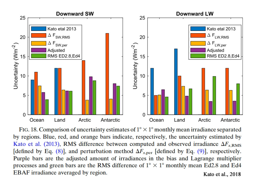
Kato et al., 2018     The uncertainty in surface irradiances over ocean, land, and polar regions at various spatial scales are estimated. The uncertainties in all-sky global annual mean upward and downward shortwave irradiance are 3 and 4 W m2, respectively, and the uncertainties in upward and downward longwave irradiance are 3 and 6 W m2, respectively. With an assumption of all errors being independent, the uncertainty in the global annual mean surface LW 1 SW net irradiance is 8 W m2.  … The downward longwave irradiance emitted by the atmosphere is primarily sensitive to near-surface temperature and the amount of water vapor as well as cloud fraction and base height in the atmosphere. [CO2 is not mentioned as factor that downward longwave irradiance is “primarily sensitive” to.]

Zadra, 2018     All model evaluation efforts reveal differences when compared to observations. These differences may reflect observational uncertainty, internal variability, or errors/biases in the representation of physical processes. The following list represents errors that were noted specifically during the meeting: cloud microphysics—errors linked to mixed-phase, supercooled liquid cloud, and warm rain; precipitation over orography—spatial distribution and intensity errors; outstanding errors in the modeling of surface fluxes; errors in the representation of the diurnal cycle of surface temperature; errors in variability and trends in historical external forcings; challenges in the prediction of midlatitude synoptic regimes and blocking; model errors in the representation of teleconnections through inadequate stratosphere–troposphere coupling; and model biases in mean state, diabatic heating, SST; errors in meridional wind response and tropospheric jet stream impact simulations of teleconnections. MJO modeling—propagation, response to mean errors, and teleconnections; subtropical boundary layer clouds—still underrepresented and tending to be too bright in models; their variation with large-scale parameters remains uncertain; and their representation may have a coupled component/feedback; tropical cyclones—high-resolution forecasts tend to produce cyclones that are too intense, although moderate improvements are seen from ocean coupling; wind–pressure relationship errors are systematic

Moon et al., 2018     The persistence of drought events largely determines the severity of socioeconomic and ecological impacts, but the capability of current global climate models (GCMs) to simulate such events is subject to large uncertainties. …  These findings reveal systematic errors in the representation of drought persistence in current GCMs [global climate models] and suggest directions for further model improvement.

Gray et al., 2018     Compared to ship‐based CO2 flux estimates, the float‐based fluxes find significantly stronger outgassing in the zone around Antarctica where carbon‐rich deep waters upwell to the surface ocean. Although interannual variability contributes, this difference principally stems from the lack of autumn and winter ship‐based observations in this high‐latitude region. These results suggest that our current understanding of the distribution of oceanic CO2 sources and sinks may need revision and underscore the need for sustained year‐round biogeochemical observations in the Southern Ocean.

(press release)      The researchers found that a large region of the Southern Ocean near Antarctica’s sea ice released 0.36 petagrams (PgC, one billion metric tons) of carbon per year. Most of that outgassing occurred during winter months. (For comparison, global fossil-fuel burning in 2016 released 9.9 PgC.) Measurements from four other regions suggested that overall, the Southern Ocean is a weak sink that absorbs 0.08 PgC/year. Climate models tend to calculate an order of magnitude larger absorption, around 0.9 PgC/year, which is consistent with estimates from ships traversing the region primarily in summer.  … The researchers conclude that an unaccounted-for carbon sink must exist elsewhere to supplement the lower-than-expected contribution of the Southern Ocean. The study suggests that current understanding of source and sink distribution may need revision and highlights the need for sustained year-round observations.

Agarwal and Wettlaufer, 2018     The fluctuation statistics of the observed sea-ice extent during the satellite era are compared with model output from CMIP5 models using a multifractal time series method. The two robust features of the observations are that on annual to biannual time scales the ice extent exhibits white noise structure, and there is a decadal scale trend associated with the decay of the ice cover. It is shown that (i) there is a large inter-model variability in the time scales extracted from the models, (ii) none of the models exhibits the decadal time scales found in the satellite observations, (iii) five of the 21 models [24%] examined exhibit the observed white noise structure, and (iv) the multi-model ensemble mean exhibits neither the observed white noise structure nor the observed decadal trend.

Simpson and Deser, 2018     Multidecadal variability in the North Atlantic jet stream in general circulation models (GCMs) is compared with that in reanalysis products of the twentieth century.  … This analysis reveals a fundamental mismatch between late winter jet stream variability in observations and GCMs [general circulation models] and a potential source of long-term predictability of the late winter Atlantic atmospheric circulation.

Urban Heat Island: Raising Surface Temperatures Artificially

Han et al., 2018     In all three regions, the stations surrounded by large urban land tend to experience rapid warming, especially at minimum temperature. This dependence is particularly significant in the southeast region, which experiences the most intense urbanization. In the northwest and intermediate regions, stations surrounded by large cultivated land encounter less warming during the main growing season, especially at the maximum temperature changes. These findings suggest that the observed surface warming has been affected by urbanization and agricultural development represented by urban and cultivated land fractions around stations in with land cover changes in their proximity and should thus be considered when analyzing regional temperature changes in mainland China.

Soon et al., 2018     [T]here is considerable evidence that, in recent decades, many instrumental records in China have been affected by warming biases caused by urbanization. So, urbanization bias may have artificially inflated the apparent warmth of the recent period [1990s-present]. This would also have the effect of artificially decreasing the relative warmth of the early period [1920s-1940s]. … The main homogenization approaches currently applied in an attempt to reduce the effects of non-climatic biases have a tendency to reduce the warmth of the early period [1920s-1940s] and increase the warmth of the recent period [1990s-present]. This has led several groups to conclude that the apparent warmth of the early period is mostly due to non-climatic biases, e.g., Li et al. (2017). On the other hand, Soon et al. (2015) note that the current homogenization approaches lead to “urban blending” when applied to a highly urbanized station network. That is, the homogenization process “aliases” (deGaetano, 2006; Pielke et al., 2007a) a fraction of the urbanization bias of urban neighbours onto the records of less urbanized station. This blending problem would have a tendency to artificially increase the warmth of the recent period and decrease the warmth of the early period.

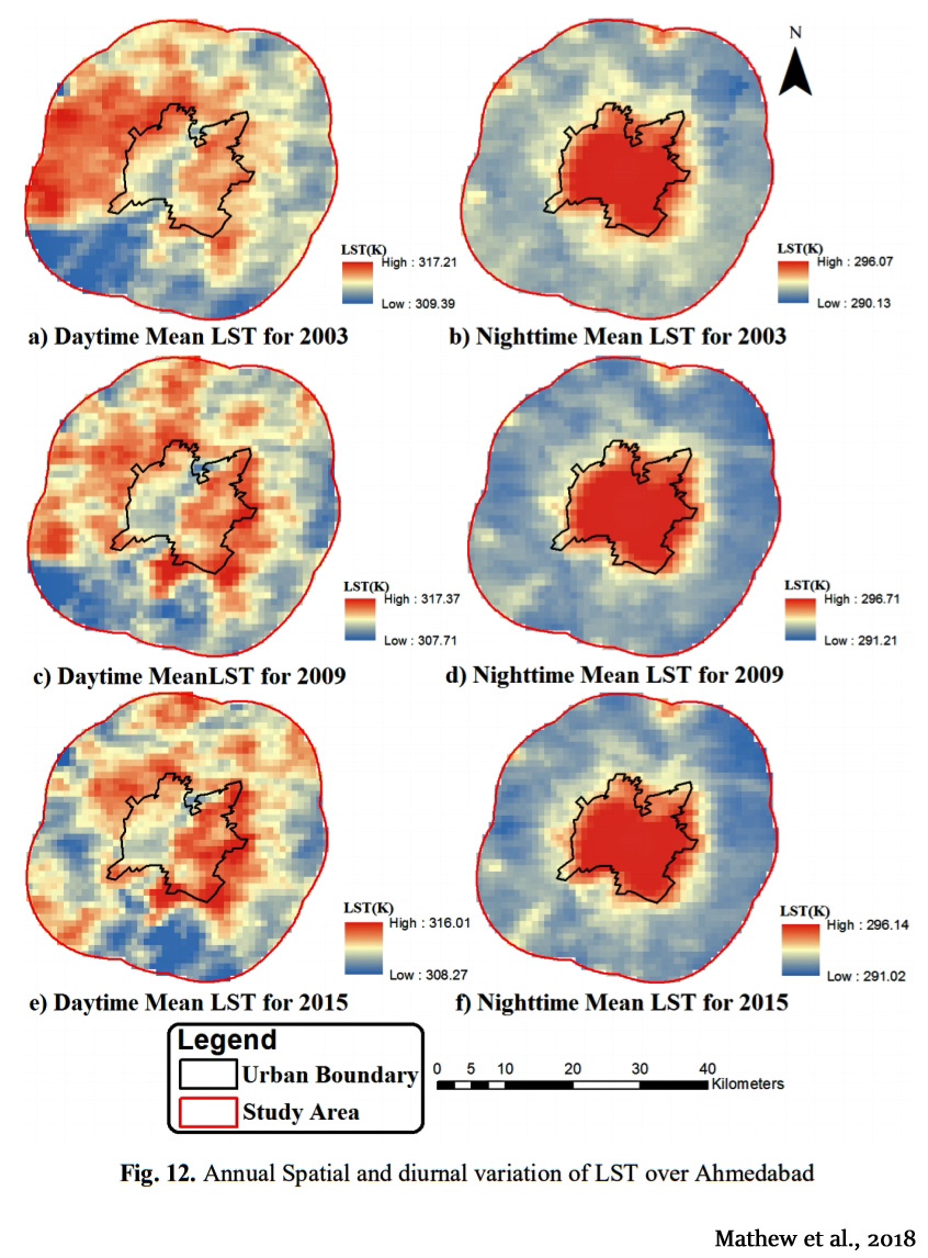
Mathew et al., 2018    Urbanization induced surface and atmospheric modifications lead to a modified thermal environment that is warmer than the neighboring rural areas, particularly at night. This phenomenon is referred as urban heat island (UHI). … Urbanization is one of the primary driving factors of land cover (LC) changes and subsequently increase of LST [land surface temperature] [Pal and Ziaul, 2016]. As an important environmental factor, LST [land surface temperature] plays a significant role in describing energy exchanges of the Earth’s land surface and atmosphere [Quattrochi et al., 1999; Weng, 2009]. LST is usually derived from thermal bands of remotely sensed data and has been considered as a primary factor for examining surface energy balance (SEB) budget [Friedl, 2002; Oke et al., 1992], assessing surface UHI (SUHI) effect [Oke, 1982; Mathew et al., 2016; Streutker, 2003; Weng and Fu, 2014; Weng et al., 2004] … Giannaros et al. [2013] have investigated that the city of Athens shows higher air temperatures than its surrounding rural areas during the night (SUHI intensity >4 K), whereas the temperature difference is less evident during early morning and mid-day hours. Observations of aerial images have confirmed that increase in albedo, such as reflective roofs, produced stronger cooling than common efforts to increase NDVI, such as green roofs, street trees and green parks [Mackey et al., 2012]. Tan and Li [2015] have observed that daytime UHI intensity is higher than the night time UHI intensity, especially for big cities. For cities with an area >100 km2 , the mean daytime UHI intensity (2.90 K) has been observed to be higher than the night time UHI intensity (2.30 K). On the basis of analysis of a large number of clusters, it has been concluded that daytime UHI intensity is more significant than night time UHI intensity for clusters with an area >2 km2 .  Lokoshchenko [2014] has studied the UHI intensity of Moscow from long term temperature records and has observed a mean UHI intensity of 1.0–1.2 K at the end of the 19th century, 1.2–1.4 K during first two decades of the 20th century and 1.6–1.8 K during both the middle and at the end of the 20th century.

Ayanlade and Howard, 2018     This study aims at estimating land use change implications on land surface temperature (LST) and heat fluxes over three cities in Niger Delta region, using satellite data. The study was carried out in three major urban areas in the Niger Delta of Nigeria: Benin City, Port Harcourt and Warri. Both in situ and satellite climatological data were used in this study to estimate the variations in heat fluxes over different land use/land cover in three major urban areas around the Niger Delta region in Nigeria. The results showed a general increased in the mean LST, with average of 1.43 °C increase between year 2004 and 2015 over different urban land use. The estimated heat flux ranges from 30.55 to 102.05 W/m2in the year 2004 but increased ranges from 33.25 to 120.06 W/m2 in the year 2015. The average heat flux was nearly 30.12 W/m2 during wet season, but much higher during the dry season with average heat flux nearly 215.75 W/m2. Increase in LST [land surface temperature] appeared to be a result of changes in landuse/landcover in the cities. The results further show that different land use exhibits a different degree of LST during both wet and dry seasons, with temperature is nearly 2 °C higher in dry season compare to wet seasons. These results imply that urban expansion in the Delta has resulted in variation in boundary currents and higher temperatures in the cities area compared to its immediate rural areas. The major findings of this study are that urban climate, urban heat redistribution and other hydrosphere processes are determined by the change in land use.

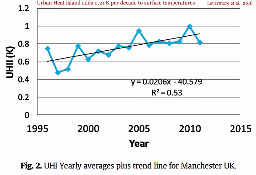
Levermore et al., 2018     This paper examines the urban heat island intensity in detail in the city of Manchester, UK [during 1996-2011]. An increasing intensity is found over time. … It was possible to assess the green space and its changes between 2000 and 2009. It can be seen that the green area has reduced by up to 11% over the whole area shown although it is only a 1.5% reduction within 200 m of the station. … Fig. 2 shows the yearly averages for UHI. There is a clear upward trend in time. The fitted trend line: UHI ¼ 0:021  YEAR−40:6 ð1Þ has a statistically significant (P b 0.1%) slope of 0.021 °C per annum [0.21°C per decade]. If this trend were to continue then over the century the UHI would be 2.42 °C. This is approximately equal to the lower predictions of climate change and is in addition to climate change. [A 1.5% to 11% reduction in green area leads to a 0.21°C per decade increase in surface temperature.]

Failing Renewable Energy, Climate Policies

DeCicco and Schlesinger, 2018      [A] major reprioritization of climate-related research, policy, and investment is urgently required, a move away from bioenergy and toward terrestrial carbon management (TCM). Researchers and policymakers must pursue actionable mitigation approaches that have the best chance of significantly reducing atmospheric CO2 concentrations in the near and medium term. … Bioenergy displaces land from prior uses, resulting in both direct and indirect land-use change. This leads to the difficult conundrum of carbon debt, i.e., the time it takes for the release of carbon stocks linked to bioenergy expansion to be paid back through future carbon uptake, which can be decades. Moreover, the realities of bioenergy production exacerbate the effects of industrial-scale agriculture on soil health, water quality, biodiversity, and other ecosystem services. … The assumption that bioenergy is inherently carbon-neutral, which is based on static forms of carbon accounting, is a major error (Haberl et al., 2012). Viewed objectively, it is quite a sweeping assumption: It asserts that a carbon flow into the atmosphere at one place and time (from bioenergy combustion) is automatically and fully offset by carbon uptake at another place and time (on ecologically productive land). Scientifically speaking, there is neither a sound basis nor a need to make this assumption. The extent to which the CO2 emitted from bioenergy use is balanced by CO2 uptake is an empirical question. … In short, a sound understanding of carbon-cycle dynamics shows that now and for the reasonably foreseeable future, the promotion of bioenergy is ill-premised for climate protection. This is particularly true if one respects the limited amount of ecologically productive land available for supplying food and fiber as well as sustaining and restoring biodiverse habitats.

Schlesinger, 2018     Recently, attention has focused on woody biomass—a return to firewood—to generate electricity. Trees remove CO2 from the atmosphere, and burning wood returns it. But recent evidence shows that the use of wood as fuel is likely to result in net CO2 emissions and may endanger forest biodiversity.

(press release)      Each year, some 7 million tons of wood pellets are shipped from the United States to Europe, where biomass fuels have been declared carbon-neutral with respect to fulfilling the commitments of the Paris Climate Accord. The current goal for the European Union (EU) is to generate 20 percent of its electricity by 2020 using renewable sources, including burning woody biomass.  In part to revive a languishing forest products industry, the U.S. Congress may also declare wood a carbon-neutral fuel. … With wood, there is the assumption, but no guarantee, that new trees will be planted and persist long enough to pay back the carbon debt created by combustion of the previous stands.  If that carbon stock is not restored, then burning wood may actually emit more CO2 to the atmosphere than burning coal. … [T]he recent science indicates that production of wood pellets for fuel is likely to put more CO2 in the atmosphere and maintain less biodiversity on the land during the next several decades.

de Oliveira Garcia et al., 2018      Increasing global woody biomass demand may cause additional pressure on forested ecosystems, enlarging negative nutrient budget areas.  … In 2014, wood and agglomerated wood products, i.e. pellets and briquettes, provided almost half (45%) of EU-28’s total inland energy production by renewables. Current European renewable energy policy will boost woody biomass demand and, considering 2015 as baseline, the global woody biomass demand is expected to be 23 × 106 t a−1 in 2024 representing a 70% increase. For 2050, global woody biomass use for energy is expected to increase by 1.6 × 1010 t a−1 (obtained from 2.3 × 1010 m3 a−1 by assuming 0.7 t m−3 as average woody biomass bulk density) representing a potential energy production ranging from 2.7–3 × 1020 J a−1 (for a 1.7–1.9 × 1010 J t−1 biomass’ energy output). By the late 21st century, the biomass energy production is expected to be 2.4–8.5 × 1020 J a−1 13, which is approximately two orders of magnitude higher than the 2016 biomass energy production of 1.8 × 1018 J a−1 14.

Krause et al., 2018     Results suggest large uncertainty in simulated future land demand and carbon uptake rates, depending on the assumptions related to land use and land management in the models. Total cumulative carbon uptake in the DGVMs [dynamic global vegetation models] is highly variable across mitigation scenarios, ranging between 19 and 130 GtC by year 2099. Only one out of the 16 combinations of mitigation scenarios and DGVMs achieves an equivalent or higher carbon uptake than achieved in the land‐use models. The large differences in carbon uptake between the DGVMs and their discrepancy against the carbon uptake in IMAGE and MAgPIE are mainly due to different model assumptions regarding bioenergy crop yields and due to the simulation of soil carbon response to land‐use change.

Scheidel et al., 2018     Efforts to combat global climate change through forestry plantations designed to sequester carbon and promote sustainable development are on the rise. This paper analyses the trajectory of Cambodia´s first large-scale reforestation project awarded within the context of climate change mitigation. The 34,007 ha concession was formally conceived to promote sustainable resource use, livelihood improvements and emission reduction. On the ground, however, vast tracks of diverse forest landscapes are being cleared and converted to acacia monocultures, existing timber stocks are logged for market sale, and customary land users dispossessed from land and forest resources. While the project adds to an ongoing land grab crisis in Cambodia, we argue that the explicit environmental ends of the forestry concession enabled a ‘green grab’ that not only exceeds the scale of land grabs caused by conventional economic land concessions, but surprisingly also exacerbates forest logging and biodiversity loss in the area. This case demonstrates the extent to which current climate change discourses, forestry agendas and their underlying assumptions require critical revision in global policy discussions to forestall the growing problem of green grabbing in land use.

Vigil, 2018     The complex impacts of climate change on human mobility have gained increased attention, but an invisible and growing number of people are also being displaced – paradoxically – by the very measures taken in the name of addressing it. Although mitigation and adaption interventions are crucial in order to decrease the likelihood of forced displacement, response measures such as agro-fuel production and carbon forest projects have been amongst the main drivers of the global land rush which is unprecedented in scale since the colonial era. These green grabs, or ‘appropriations of natural resources for environmental ends’, are serving to cleanse the image of polluters, with devastating social and environmental consequences. The logic behind market-driven initiatives is that we should ‘sell nature in order to save it’ and that unsustainable practices in one place can be repaired by sustainable ones in another. With regard to displacement, they assume that their negative effects can be balanced by the gains in environmental protection. However, and although the presence of certain entities (mostly corporations and extractive industries) is indeed negative for the environment, it is local populations and indigenous peoples – who are the best positioned to protect natural resources – that are being evicted.  Although land and green grabs are occurring worldwide, it is in countries where the protection of human rights is low, or inexistent, that they have reached the most alarming peaks. Due to a combination of international and domestic drivers, Africa has been by far the most targeted continent. Tropical forests are typically under the formal control of the government and it is relatively simple to expropriate them from inhabitants in the name of climate mitigation.

Schäfer et al., 2018     Multiple types of fluctuations impact the collective dynamics of power grids and thus challenge their robust operation.

(press release)     More renewables mean less stable grids, researchers find …  [I]ntegrating growing numbers of renewable power installations and microgrids onto the grid can result in larger-than-expected fluctuations in grid frequency.

Jewell et al., 2018     Hopes are high that removing fossil fuel subsidies could help to mitigate climate change by discouraging inefficient energy consumption and levelling the playing field for renewable energy.  Here we show that removing fossil fuel subsidies would have an unexpectedly small impact on global energy demand and carbon dioxide emissions and would not increase renewable energy use by 2030. Removing subsidies in most regions would deliver smaller emission reductions than the Paris Agreement (2015) climate pledges and in some regions global subsidy removal may actually lead to an increase in emissions, owing to either coal replacing subsidized oil and natural gas or natural-gas use shifting from subsidizing, energy-exporting regions to non-subsidizing, importing regions.

Cradden and McDermott, 2018     Prolonged cold spells were experienced in Ireland in the winters of 2009–10 and 2010–11, and electricity demand was relatively high at these times, whilst wind generation capacity factors were low. Such situations can cause difficulties for an electricity system with a high dependence on wind energy.

Blazquez et al., 2018     However, promoting renewables –in liberalized power markets– creates a paradox in that successful penetration of renewables could fall victim to its own success. With the current market architecture, future deployment of renewable energy will necessarily be more costly and less scalable. Moreover, transition towards a full 100% renewable electricity sector is unattainable. Paradoxically, in order for renewable technologies to continue growing their market share, they need to co-exist with fossil fuel technologies. … The paradox is that the same market design and renewables policies that led to current success become increasingly less successful in the future as the share of renewables in the energy mix grows. … Full decarbonization of a power sector that relies on renewable technologies alone, given the current design of these markets, is not possible as conventional technologies provide important price signals. Markets would collapse if the last unit of fossil fuel technologies was phased out. In the extreme (theoretical) case of 100 percent renewables, prices would be at the renewables marginal cost, equal to zero or even negative for long periods. These prices would not be capturing the system’s costs nor would they be useful to signal operation and investment decisions. The result would be a purely administered subsidy, i.e., a non-market outcome. This is already occurring in Germany as Praktiknjo and Erdmann [31] point out and is clearly an unstable outcome. Thus, non-dispatchable technologies need to coexist with fossil fuel technologies. This outcome makes it impossible for renewables policy to reach success, defined as achieving a specified level of deployment at the lowest possible cost. With volatile, low and even negative electricity prices, investors would be discouraged from entering the market and they would require more incentives to continue to operate.

Marques et al., 2018     The installed capacity of wind power preserves fossil fuel dependency. … Electricity consumption intensity and its peaks have been satisfied by burning fossil fuels. … [A]s RES [renewable energy sources] increases, the expected decreasing tendency in the installed capacity of electricity generation from fossil fuels, has not been found. Despite the high share of RES in the electricity mix, RES, namely wind power and solar PV, are characterised by intermittent electricity generation.  … The inability of RES-I [intermittent renewable energy sources like wind and solar] to satisfy high fluctuations in electricity consumption on its own constitutes one of the main obstacles to the deployment of renewables. This incapacity is due to both the intermittency of natural resource availability, and the difficulty or even impossibility of storing electricity on a large scale, to defer generation.  As a consequence, RES [renewable energy sources] might not fully replace fossil sources … The literature proves the existence of a unidirectional causality running from RES [renewable energy sources] to NRES [non-renewable energy sources] (Almulali et al., 2014; Dogan, 2015; Salim et al., 2014). This unidirectional causality proves the need for countries to maintain or increase their installed capacity of fossil fuel generation, because of the characteristics of RES production. …  In fact, the characteristics of electricity consumption reinforce the need to burn fossil fuels to satisfy the demand for electricity. Specifically, the ECA results confirm the substitution effect between the installed capacity of solar PV and fossil fuels. In contrast, installed wind power capacity has required all fossil fuels and hydropower to back up its intermittency in the long-run equilibrium. The EGA outcomes show that hydropower has been substituting electricity generation through NRES [non-renewable energy sources], but that other RES have needed the flexibility of natural gas plants, to back them up. … [D]ue to the intermittency phenomenon, the growth of installed capacity of RES-I [intermittent renewable energy sources – wind power] could maintain or increase electricity generation from fossil fuels.  … In short, the results indicate that the EU’s domestic electricity production systems have preserved fossil fuel generation, and include several economic inefficiencies and inefficiencies in resource allocation. … [A]n increase of 1% in the installed capacity of wind power provokes an increase of 0.26%, and 0.22% in electricity generation from oil and natural gas, respectively in the long-run.

Sterman et al., 2018     [G]overnments around the world are promoting biomass to reduce their greenhouse gas (GHG) emissions. The European Union declared biofuelsto be carbon-neutral to help meet its goal of 20% renewable energy by 2020, triggering a surge in use of wood for heat and electricity (European Commission 2003, Leturcq 2014, Stupak et al 2007). … But do biofuels actually reduce GHG emissions? … [A]lthough wood has approximately the same carbon intensity as coal (0.027 vs. 0.025 tC GJ−1 of primary energy […]), combustion efficiency of wood and wood pellets is lower (Netherlands Enterprise Agency; IEA 2016). Estimates also suggest higher processing losses in the wood supply chain (Roder et al 2015). Consequently, wood-fired power plants generate more CO2 per kWh than coal. Burning wood instead of coal therefore creates a carbon debt—an immediate increase in atmospheric CO2 compared to fossil energy—that can be repaid over time only as—and if— NPP [net primary production] rises above the flux of carbon from biomass and soils to the atmosphere on the harvested lands. … Growth in wood supply causes steady growth in atmospheric CO2 because more CO2 is added to the atmosphere every year in initial carbon debt than is paid back by regrowth, worsening global warming and climate change. The qualitative result that growth in bioenergy raises atmospheric CO2 does not depend on the parameters: as long as bioenergy generates an initial carbon debt, increasing harvests mean more is ‘borrowed’ every year than is paid back. More precisely, atmospheric CO2 rises as long as NPP [net primary production] remains below the initial carbon debt incurred each year plus the fluxes of carbon from biomass and soils to the atmosphere. … [C]ontrary to the policies of the EU and other nations, biomass used to displace fossil fuels injects CO2 into the atmosphere at the point of combustion and during harvest, processing and transport. Reductions in atmospheric CO2 come only later, and only if the harvested land is allowed to regrow.

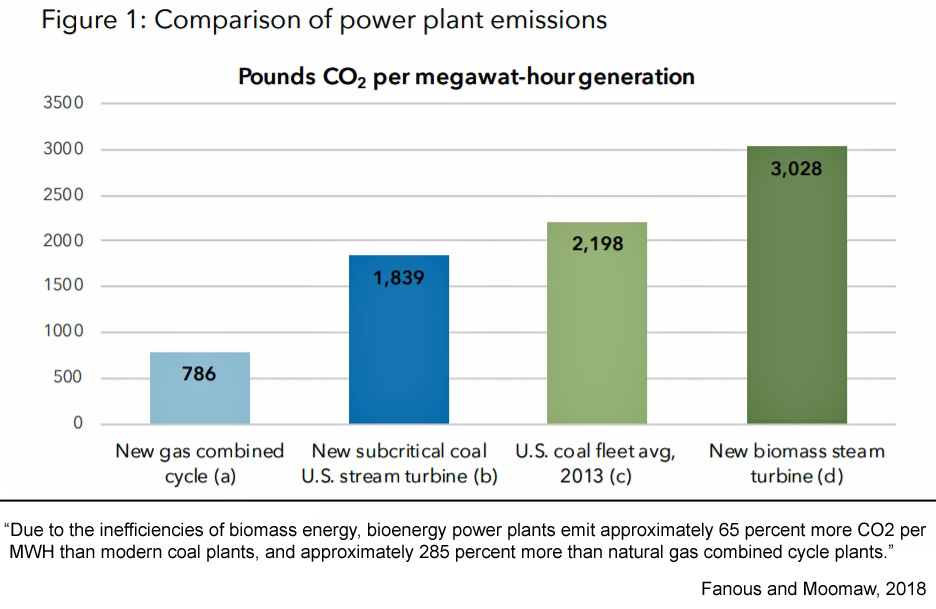
Fanous and Moomaw, 2018    These nations fail to recognize the intensity of CO2 emissions linked to the burning of biomass. The chemical energy stored in wood is converted into heat or electricity by way of combustion and is sometimes used for combined heat and power cogeneration. At the point of combustion, biomass emits more carbon per unit of heat than most fossil fuels. Due to the inefficiencies of biomass energy, bioenergy power plants emit approximately 65 percent more CO2, per MWH than modern coal plants, and approximately 285 percent more than natural gas combined cycle plants. Furthermore, the Intergovernmental Panel on Climate Change (IPCC) states that combustion of biomass generates gross greenhouse gas (GHG) emissions roughly equivalent to the combustion of fossil fuels. In the case of forest timber turned into wood pellets for bioenergy use, the IPCC further indicates that the process produces higher CO2 emissions than fossil fuels for decades to centuries.

Lee and Jung, 2018     The results of the autoregressive distributed lag bounds test show that renewable energy consumption has a negative effect on economic growth, and the results of a vector error correction mechanism causality tests indicate a unidirectional relationship from economic growth to renewable energy consumption. The empirical results imply that economic growth is a direct driver expanding renewable energy use. In terms of policy implications, it is best for policy makers to focus on overall economic growth rather than expanding renewable energy to drive economic growth. … [O]ur result suggests that renewable energy policy should be implemented when the real GDP is enough large to overcome the negative impact from renewable energy, because the causality from economic growth to renewable energy consumption in the long run as one of our result is caused by both low productivity of renewable energy production and expansion of government-led renewable energy.

Moomaw, 2018     The European Union aims to replace fossil fuels with renewable energy, but ignores the fact that burning wood from forests releases carbon dioxide. Instead, bioenergy emissions are officially counted as zero or carbon neutral. … The Intergovernmental Panel on Climate Change summarized the emissions of bioenergy use as follows: “The combustion of biomass generates gross GHG emissions roughly equivalent to the combustion of fossil fuels.”  When wood is burned to produce electricity, it releases an estimated 80% more carbon dioxide per unit of electricity than coal. This work by Dr. Sterman of MIT and his colleagues provides the first quantitative comparison of the total carbon emissions from forest bioenergy throughout the full carbon cycle, and compares them to coal, and renewables for a variety of bioenergy scenarios. … Burning wood to make electricity is also far more costly than deploying solar or wind technologies, and is only made economic by the European governments billions of dollars in annual subsidies. … A 2016 study found that 45% of EU renewable energy was from burning wood, and by 2020 the amount would equal the total EU harvest.  According to an analysis of the new EU directive, conducted at Princeton University, “To supply even one third of the additional renewable energy likely required by 2030, Europe would need to burn an amount of wood greater than its total harvest today.”

Miller and Keith, 2018     We find that generating today’s US electricity demand (0.5 TW e) with wind power would warm Continental US surface temperatures by 0.24°C. Warming arises, in part, from turbines redistributing heat by mixing the boundary layer. Modeled diurnal and seasonal temperature differences are roughly consistent with recent observations of warming at wind farms, reflecting a coherent mechanistic understanding for how wind turbines alter climate. The warming effect is: small compared with projections of 21st century warming, approximately equivalent to the reduced warming achieved by decarbonizing global electricity generation, and large compared with the reduced warming achieved by decarbonizing US electricity with wind. For the same generation rate, the climatic impacts from solar photovoltaic systems are about ten times smaller than wind systems. Wind’s overall environmental impacts are surely less than fossil energy. Yet, as the energy system is decarbonized, decisions between wind and solar should be informed by estimates of their climate impacts.

(press release)    A new study by a pair of Harvard researchers finds that a high amount of wind power could mean more climate warming, at least regionally and in the immediate decades ahead. The paper raises serious questions about just how much the United States or other nations should look to wind power to clean up electricity systems. … The study, published in the journal Joule, found that if wind power supplied all US electricity demands, it would warm the surface of the continental United States by 0.24˚C. That could significantly exceed the reduction in US warming achieved by decarbonizing the nation’s electricity sector this century, which would be around 0.1˚C.

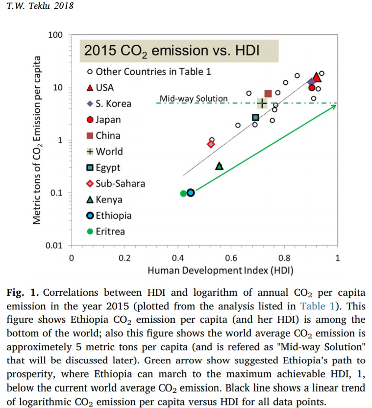
Teklu, 2018     In this study, it is argued, Ethiopia should in principle agree with the World in international climate change agreements (such as the Paris climate accord), purely to avoid any political and economic sanctions from “Earth friendly” nations and institutions; however, [Ethopia] should avoid becoming carbon neutral at the expense of adding costs and slowing her industrial development prospects. In fact, since CO2 emission (energy consumption) is directly correlated to economic prosperity and industrialization (see Table 1 and Figure 1), Ethiopia should plan to increase her CO2 emission per capita as much as possible. Ethiopia should understand that climate agreements such as the Paris accord are designed and destined to fail. Hence, Ethiopia should avoid carbon-tax, different form of financial aid, poverty-trap; instead she should plan on how to live with the inevitable global atmospheric CO2 concentration increase. The same is true for majority of least developed countries (LDCs). Global climate change [as an] issue could be a neo-colonialism and neo-cold-war instrument designed by neo-liberal institutions; hence, if Ethiopia is willing to confront any political and economic burden from “Earth friendly” nations and institutions, Ethiopia should lead other Africans’ towards the mid-way solution; and if “Earth friendly” countries does not agree with such just and simple solution; then, Ethiopia should lead Africa, in following USA, and exit from the Paris climate accord. In doing so, Ethiopia may repeat the leadership role she played during African decolonization struggle.

Miller and Keith, 2018     Power density is the rate of energy generation per unit of land surface area occupied by an energy system. The power density of low-carbon energy sources will play an important role in mediating the environmental consequences of energy system decarbonization as the world transitions away from high power-density fossil fuels. All else equal, lower power densities mean larger land and environmental footprints. The power density of solar and wind power remain surprisingly uncertain: estimates of realizable generation rates per unit area for wind and solar power span 0.3–47 We m−2 and 10–120 We m−2 respectively. We refine this range using US data from 1990–2016. We estimate wind power density from primary data, and solar power density from primary plant-level data and prior datasets on capacity density. The mean power density of 411 onshore wind power plants in 2016 was 0.50 We m−2. Wind plants with the largest areas have the lowest power densities. Wind power capacity factors are increasing, but that increase is associated with a decrease in capacity densities, so power densities are stable or declining. If wind power expands away from the best locations and the areas of wind power plants keep increasing, it seems likely that wind’s power density will decrease as total wind generation increases. The mean 2016 power density of 1150 solar power plants was 5.4 We m−2. Solar capacity factors and (likely) power densities are increasing with time driven, in part, by improved panel efficiencies. Wind power has a 10-fold lower power density than solar, but wind power installations directly occupy much less of the land within their boundaries. The environmental and social consequences of these divergent land occupancy patterns need further study. … Power densities clearly carry implications for land use. Meeting present-day US electricity consumption, for example, would require 12% of the Continental US land area [about 350,000 square miles or 912,000 square kilometers] for wind at 0.5 We m−2, or 1% for solar at 5.4 We m−2.

Wind Power Harming The Environment, Biosphere

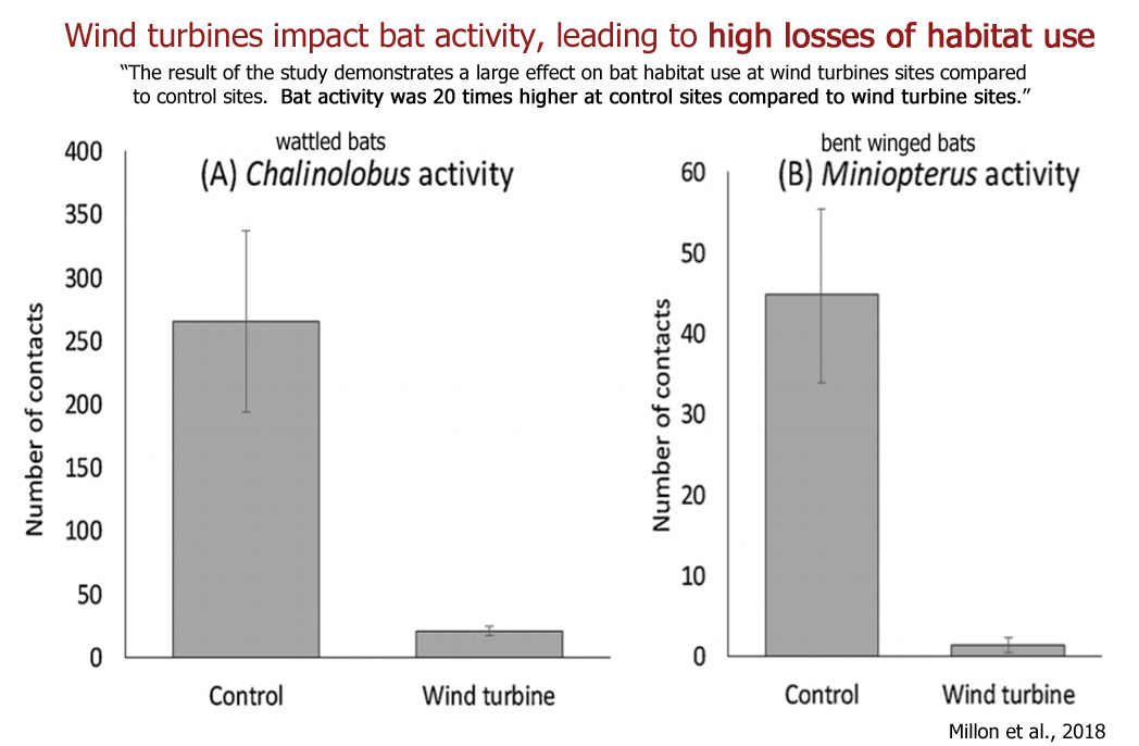
Millon et al., 2018 (full paper)    Wind turbines impact bat activity, leading to high losses of habitat use … Island bats represent 60% of bat species worldwide and the highest proportion of terrestrial mammals on isolated islands, including numerous endemic and threatened species (Fleming and Racey, 2009). … We present one of the first studies to quantify the indirect impact of wind farms on insectivorous bats in tropical hotspots of biodiversity. Bat activity [New Caledonia, Pacific Islands, which hosts nine species of bat] was compared between wind farm sites and control sites, via ultrasound recordings at stationary points [A bat pass is defined as a single or several echolocation calls during a five second interval.] The activity of bent winged bats (Miniopterus sp.) and wattled bats (Chalinolobus sp.) were both significantly lower at wind turbine sites. The result of the study demonstrates a large effect on bat habitat use at wind turbines sites compared to control sites. Bat activity was 20 times higher at control sites compared to wind turbine sites, which suggests that habitat loss is an important impact to consider in wind farm planning. …  Here, we provide evidence showing that two genera of insectivorous bat species are also threatened by wind farms.  … To our knowledge, this is one of the first studies quantifying the indirect negative impact of wind turbines on bat activity in the tropics. … The lower attractiveness of the foraging habitat under wind turbines, both in a tropical and in a temperate climate, indicates that the indirect impact of wind turbine is a worldwide phenomenon.

Lopucki et al., 2018     Living in habitats affected by wind turbines may result in an increase in corticosterone levels in ground dwelling animals … Environmental changes and disturbance factors caused by wind turbines may act as potential stressors for natural populations of both flying and ground dwelling animal species. The physiological stress response results in release of glucocorticoid hormones. … The common vole showed a distinct physiological response − the individuals living near the wind turbines had a higher level of corticosterone [physiological stress affecting regulation of energy, immune reactions]. … This is the first study suggesting impact of wind farms on physiological stress reactions in wild rodent populations. Such knowledge may be helpful in making environmental decisions when planning the development of wind energy and may contribute to optimization of conservation actions for wildlife.

Ferrão da Costa et al., 2018     According to a review by Lovich and Ennen (2013), the construction and operation of wind farms have both potential and known impacts on terrestrial vertebrates, such as: (i) increase in direct mortality due to traffic collisions; (ii) destruction and modification of the habitat, including road development, habitat fragmentation and barriers to gene flow; (iii) noise effects, visual impacts, vibration and shadow flicker effects from turbines; (iv) electromagnetic field generation; (v) macro and microclimate change; (vi) predator attraction; and (vii) increase in fire risks. … Helldin et al. (2012) also highlighted that the development of road networks associated with wind farms could promote increased access for traffic related to recreation, forestry, agriculture and hunting. The consequence, particularly on remote places, is the increase in human presence, affecting large mammals via significant disturbance, habitat loss and habitat fragmentation. These negative effects are expected to be particularly relevant for species that are more sensitive to human presence and activities, such as large carnivores. Large carnivores, such as the wolf, bear, lynx or wolverine, tend to avoid areas that are regularly used by humans and—especially for breeding—show a preference for rugged and undisturbed areas (Theuerkauf et al. 2003; George and Crooks 2006; May et al. 2006; Elfstrom et al. 2008; Sazatornil et al. 2016), which are often chosen for wind power development (Passoni et al. 2017). … Results have shown that the main impact of wind farms on wolves is the induced reduction on breeding site fidelity and reproductive rates. These effects, particularly when breeding sites shift to more unsuitable areas, may imply decreasing survival and pack viability in the short term.

Watson et al., 2018     The global potential for wind power generation is vast, and the number of installations is increasing rapidly. We review case studies from around the world of the effects on raptors of wind-energy development. Collision mortality, displacement, and habitat loss have the potential to cause population-level effects, especially for species that are rare or endangered.

Aschwanden et al., 2018     The extrapolated number of collisions was 20.7 birds/wind turbine (CI-95%: 14.3–29.6) for 8.5 months. Nocturnally migrating passerines, especially kinglets (Regulus sp.), represented 55% of the fatalities. 2.1% of the birds theoretically exposed to a collision (measured by radar at the height of the wind turbines) were effectively colliding.

Naylor, 2018     While wind energy provides a viable solution for emission reductions, it comes at an environmental cost, particularly for birds. As wind energy grows in popularity, its environmental impacts are becoming more apparent. Recent studies indicate that wind power has negative effects on proximate wildlife. These impacts can be direct—collision fatalities—and indirect—habitat loss (Fargione et al. 2012; Glen et al. 2013). Negative impacts associated with operational wind farms include collision mortalities from towers or transmission lines and barotrauma for bats. Habitat loss and fragmentation, as well as avoidance behavior, are also consequences resulting from wind farm construction and related infrastructure. The potential harm towards protected and migratory bird species are an urgent concern, especially for wind farms located along migratory flyways. In terms of mortality, wind turbines kill an estimated 300,000 to 500,000 birds, annually (Smallwood 2013). The high speed at which the fan wings move and the concentration of turbines create a gauntlet of hazards for birds to fly through. … [T]he height of most wind turbines aligns with the altitude many bird species fly at (Bowden 2015). Birds of prey— raptors—are of particular concern because of their slow reproductive cycles and long lifespans relative to other bird species (Kuvlesky 2007).

Lange et al., 2018     Results from our surface water extractions and aerial surveys suggest that the wind farm has negatively affected redheads through altered hydrology and disturbance displacement. Our surface water extraction analysis provides compelling evidence that the local hydrology has been greatly affected by the construction of the wind farm. … Our results suggest the occurrence of direct habitat loss and disturbance displacement of redheads from the wind farm along the lower Texas coast. Although our study was directed solely toward redheads, it is likely that this wind farm has affected other species that use these wetlands or migrate along the lower Texas coast (Contreras et al. 2017). Studies in Europe investigating the effects on waterfowl by wind turbines have reported similar results, showing that turbines have likely compromised foraging opportunities for waterfowl through disturbance displacement (Larsen and Madsen 2000).

Barry et al., 2018     The findings indicate that residential proximity to wind turbines is correlated with annoyance and health-related quality of life measures. These associations differ in some respects from associations with noise measurements. Results can be used to support discussions between communities and wind-turbine developers regarding potential health effects of wind turbines.

Chiebáo, 2018     I studied the large-scale movements of white-tailed eagles during the dispersal period, assessing their space use in relation to the distribution of existing and proposed wind farms across Finland. I found that a breeding pair holding a territory closer to an installation has a lower probability to breed successfully when compared to a pair from a territory lying farther away. Such lower probability may in part reflect a harmful interaction between the eagles and wind turbines in the form of collision mortality, to which the adults appear to be particularly vulnerable during the breeding season. Regarding the post-fledging period, I found that the probability of a young eagle approaching a wind turbine decreases sharply as the turbine is installed at increasing distances from the nest.

Shakespear, 2018     A trend was found, whereby developing countries tend to suffer the most socio-environmental disruption from material extraction for solar-panels and wind-turbines while exhibiting lower implementation of these technologies, and developed countries show opposite effects. This indicates that EUE [ecologically unequal exchange] effects constitute global solar-panel and wind-turbine systems, and that developed countries displace socio-environmental disruption from energy innovation onto developing countries. … [I]mplementation of solarpanels and wind-turbines tended to be the most prevalent within countries that suffer the least environmental and socio-economic consequences from the extraction of materials for these technologies. This effectively means that efforts to increase sustainability in relatively powerful countries via renewable energy implementation exacerbates unsustainable practices in the relatively less powerful countries that extract the minerals for these technologies.

Barré et al., 2018     Wind energy is rapidly growing as a renewable source of energy but is not neutral for wildlife, especially bats. Whereas most studies have focused on bat mortality through collision, very few have quantified the loss of habitat use resulting from the potential negative impact of wind turbines … We quantified the impact of wind turbines at different distances on the activity of 11 bat taxa and 2 guilds. … We found a significant negative effect of proximity to turbines on activity for 3 species (Barbastella barbastellus, Nyctalus leisleiri, Pipistrellus pipistrellus), 2 species-groups (Myotis spp., Plecotus spp.) and 2 guilds (fast-flying and gleaner). … The current situation is particularly worrying, with 89% of 909 turbines established in a region that does not comply with recommendations, which themselves are far from sufficient to limit the loss of habitat use. … [T]here is an urgent need to assess the potential decrease in bat activity close to wind turbines in order to quantify the changes of habitat use and the distance of impact. This possible underestimated impact of wind turbines could constitute an important concern, affecting population dynamics with a loss of habitat availability (Rodrigues et al., 2015). … [F]or most species, the negative effect of wind turbines on activity extends at least 1000 m from a wind turbine. The lost activity was therefore likely underestimated and occurred at > 1000 m. Thus, the percentage of lost activity was high, even at long-distances: for instance, at 500 m from the nearest turbine, we detected activity losses of 57% and 77% for P. pipistrellus and the gleaner species guild, respectively (Fig. 3). … Among the 909 wind turbines in northwest France, which contained the studied farms, 89% were established at < 200 m from any type of wooded edges (forest or hedgerows).

Thaker et al., 2018     [W]e find that wind farms reduce the abundance and activity of predatory birds (for example, Buteo,  Butastur and Elanus species), which consequently increases the density of lizards, Sarada superba. … [W]e find that wind farms have emerging impacts that are greatly underestimated. There is thus a strong need for an ecosystem-wide view when aligning green-energy goals with environment protection.

(press release)      Wind farms act as a top “predator” in some ecosystems, harming birds at the top of the food chain and triggering a knock-on effect overlooked by green energy advocates, scientists said Monday. … Close to 17 million hectares—an area roughly the size of Tunisia—is currently used for generating wind energy worldwide, and researchers warned that developers had “greatly underestimated” the impact the technology has on wildlife. In new research, an international team of scientists studied the effects of wind turbine use in the Western Ghats, a UNESCO-listed range of mountains and forest spanning India’s west coast region and a global “hotspot” of biodiversity. They found that predatory raptor birds were four times rarer in areas of plateau where wind turbines were present, a disruption that cascaded down the food chain and radically altered the density and behaviour of the birds’ prey. … Wind farms are known to be harmful to birds, disrupting their migration patterns and causing above average death rates. Thaker said her research, published in the journal Nature Ecology & Evolution, showed that wind farms replicated the role of the top predator in the food chain by keeping the raptors at bay. “They trigger changes to the balance of animals in an ecosystem as if they were top predators,” she said.

Ishitake, 2018     We investigated whether long-term exposure to low-frequency noise generated by wind power facilities is a risk factor for sleep disorders. We performed an epidemiological study of the living environment and health effects of such noise by surveying 9,000 residents (≥20 years of age) living in areas with operational wind power facilities. Sleep disorders were assessed using the Athens Insomnia Scale. To assess environmental noise in residential areas near wind turbines, infrasound and low-frequency sound exposure levels were measured at 50 community centers of a town. The prevalence of sleep disorders was significantly higher among residents who reported subjectively hearing noise (by approximately twofold) than among those who did not. Moreover, the reported prevalence of sleep disorders was significantly higher (by approximately twofold) among residents living at a distance of ≤1,500 m from the nearest wind turbine than among residents living at a distance of ≥2,000 m, suggesting a dose-response relationship. The attitudes of residents towards wind power facilities strongly affected their responses regarding sleep disorder prevalence. It is highly likely that audible noise generated by wind power facilities is a risk factor for sleep disorders. Obtaining a satisfactory consensus from local residents before installing wind power facilities is important as for more amenable their attitudes towards such facilities.

Jensen et al., 2018     We present the results of a large-scale analysis on how on-shore and off-shore wind turbines affect the property prices of nearby single family residential and vacation homes in Denmark. We find that on-shore wind turbines negatively affect the price of surrounding properties to a distance of three kilometers. The negative impact increases with the number of wind turbines at a declining marginal rate but declines with distance. In the case of off-shore wind turbine farms, we do not find a significant effect of having an off-shore wind farm in view from a property itself or from the nearest beach, likely because the closest off-shore turbine is 9 km from the closest traded home. … The results suggest that ceteris paribus, wind turbine farms should be built quite far away from residential areas with turbines gathered in larger wind farms rather than installed as single turbines.

Michaud et al., 2018     An aggregate annoyance construct has been developed to account for annoyance that ranges from not at all annoyed to extremely annoyed, toward multiple wind turbine features. The practical value associated with aggregate annoyance would be strengthened if it was related to health. The objective of the current paper was to assess the association between aggregate annoyance and multiple measures of health. … The average aggregate annoyance score for participants who indicated they had a health condition (e.g., chronic pain, Pittsburgh Sleep Quality Index (PSQI) > 5, tinnitus, migraines/headaches, dizziness, highly sensitive to noise, and reported a high sleep disturbance) ranged from 2.53 to 3.72; the mean score for those who did not report these same conditions ranged between 0.96 and 1.41. Household complaints about wind turbine noise had the highest average aggregate annoyance (8.02), compared to an average of 1.39 among those who did not complain. … It should also be underscored that in response to concerns raised during the external peer review of this paper, the association between the non-noise annoyance variables and self-reported and measured health outcomes was evaluated. With the exception of vibration annoyance, which could not be evaluated due to the small sample size, blinking lights, shadow flicker, and visual annoyance were found to be statistically associated with several measures of health, including, but not limited to, migraines, dizziness, tinnitus, chronic pain, sleep disturbance, perceived stress, quality of life measures, lodging a WTN-related complaint, and measured diastolic blood pressure.

Pawlaczyk-Łuszczyńska et al., 2018     The aim of this study was to evaluate the perception and annoyance of noise from wind turbines in populated areas of Poland. A questionnaire inquiry was carried out among 517 subjects, aged 18–88, living within 204–1726 m from the nearest wind turbine. For areas where respondents lived, A-weighted sound pressure levels (SPLs) were calculated as the sum of the contributions from the wind power plants in the specific area. It has been shown that the wind turbine noise at the calculated A-weighted SPL of 33–50 dB was perceived as annoying or highly annoying by 46% and 28% of respondents, respectively. Moreover, 34% and 18% of them said that they were annoyed or highly annoyed indoors, respectively. The perception of high annoyance was associated with the A-weighted sound pressure level or the distance from the nearest wind turbine, general attitude to wind farms, noise sensitivity and terrain shape (annoyance outdoors) or road-traffic intensity (annoyance indoors). About 48–66% of variance in noise annoyance rating might be explained by the aforesaid factors. It was estimated that at the distance of 1000 m the wind turbine noise might be perceived as highly annoying outdoors by 43% and 2% of people with negative and positive attitude towards wind turbines, respectively. There was no significant association between noise level (or distance) and various health and well-being aspects. However, all variables measuring health and well-being aspects, including stress symptoms, were positively associated with annoyance related to wind turbine noise.

Dunlap, 2018      The ‘solution’ is now the ‘problem:’ wind energy, colonisation and the ‘genocide-ecocide nexus’ … The green economy emerges in the shadow of conventional fossil fuel production, presenting itself as a ‘solution’ and pathway to slow the effects of ecological, climate and economic crisis. Said differently, renewable energy in particular, and the green economy in general, emerge as the ‘lesser evil’ of industrial development. Discussing the principle of ‘lesser evil’, Eyal Weizman writes, ‘less brutal measures are also those that may be more easily naturalised, accepted and tolerated – and hence more frequently used, with the result that a greater evil may be reached cumulatively’. The green economy is the lesser industrial evil, utilising a technique of war to morally buffer and continue the proliferation of industrial waste in the name of climate change mitigation, which according to this research results in greater cumulative social and environmental alterations and, even, the systemic and increasing destruction of alternative value systems and ways of life valuing their relationships with their ecosystems. … State-sanctioned land grabbing by corporations in the name of sustainable development is accumulation by dispossession by environmental ethic – green grabbing [Fairhead et al., 2012] – which walks a fine line with genocide. ‘The Rana’, exclaims: ‘We hold responsible all of the political parties of Mexico, the government in its different levels for the attempt to annihilate us, the attempt to grab our land and to wipe us off the map.’

Dunlap, 2018     Sustainable development and climate change mitigation policies, Dunlap and Fairhead argue, have instigated and renewed old conflicts over land and natural resources, deploying military techniques of counterinsurgency to achieve land control. Wind energy development, a popular tool of climate change mitigation policies, has consequently generated conflict in the Isthmus of Tehuantepec (Istmo) region in Oaxaca, Mexico. Research is based on participant observation and 20 recorded interviews investigating the Fuerza y Energía Bíi Hioxo Wind Farm on the outskirts of Juchitán de Zaragoza. This paper details the repressive techniques employed by state, private and informal authorities against popular opposition to the construction of the Bíi Hioxo wind park on communal land. Providing background on Juchitán, social property and counterinsurgency in Southern Mexico, this paper analyzes the development of the Bíi Hioxo wind park. It further explores the emergence of ‘hard’ and ‘soft’ counterinsurgency techniques used to pacify resistance against the wind park, enabling its completion next to the Lagoon Superior in October 2014. Discussing the ‘greening of counterinsurgency’, this contribution concludes that the Bíi Hioxo wind park has spawned social divisions and violent conflict, and intervened in the sensitive cultural fabric of Istmeño life.

Tonin, 2018     In 2015, the Australian Senate Select Committee on Wind Turbines concluded there was credible evidence from a number of people who reside in proximity to wind turbines who have complained of a range of adverse health impacts. These include tinnitus, raised blood pressure, heart palpitations, tachycardia, stress, anxiety, vertigo, dizziness, nausea, blurred vision, fatigue, cognitive dysfunction, headaches, ear pressure, exacerbated migraine disorders, motion sensitivity, inner ear damage and sleep deprivation.  A historical review shows that whilst initially the audible sounds of wind turbines disturbed people in their sleep, more complex prognoses such as Vibroacoustic Disease and Wind Turbine Syndrome were proposed to explain the reported health symptoms. These diseases were hypothesised to be linked to the emission of infrasound from wind turbines, particularly tonal infrasound at the blade pass frequency of the turbine blades and associated harmonics. … Salt [2014] disagrees with the proposition that “what you can’t hear can’t affect you”. In his proposal, it is the outer hair cells (OHC) in the cochlear that are stimulated by infrasound as opposed to the inner hair cells (IHC) which are responsible for audible hearing. Figure 12 is a cross section through the cochlear in the inner ear and the location of the Organ of Corti containing the OHC and the IHC. Figure 13 is a more detailed view of the Organ of Corti.  According to Salt, the ear responds to infrasound through the OHC and whilst the sensation is not “heard”, there is nevertheless a stimulation of the cochlea. The question is whether the stimulation by infrasound remains confined to the ear and has no other influence on the person or whether there are on-flowing effects which would explain the symptoms allegedly attributable to wind turbine infrasound.  … Pierpont coined the term “Wind Turbine Syndrome” to explain the symptoms of persons exposed to infrasound from wind turbines including “a feeling of internal pulsation, quivering or jitteriness, and it is accompanied by nervousness, anxiety, fear, a compulsion to flee or check the environment for safety, nausea, chest tightness, and tachycardia”. According to Van den Berg [56], these symptoms are well known when persons are put under stress and thus might not be specific to the impact of wind turbines. People with a generalised anxiety disorder also have symptoms which include trembling, restlessness or a feeling of being “edgy”, excessive worry and tension, an unrealistic view of problems, nausea and muscle tension and these conditions might become worse during periods of stress.

Elevated CO2: Greens Planet, Higher Crop Yields

Pau et al., 2018     Long-term increases in tropical flowering activity across growth forms in response to rising CO2 and climate change … Here, we analyze a 28-year record of tropical flower phenology in response to anthropogenic climate and atmospheric change. We show that a multidecadal increase in flower activity is most strongly associated with rising atmospheric CO2 concentrations using yearly aggregated data. Compared to significant climatic factors, CO2 had on average an approximately three-, four-, or fivefold stronger effect than rainfall, solar radiation, and the Multivariate ENSO Index, respectively.

Zeng et al., 2018     Leaf area index (LAI) is increasing throughout the globe, implying the Earth greening. Global modelling studies support this contention, yet satellite observations and model simulations have never been directly compared. Here, for the first time, we used a coupled land-climate model to quantify the potential impact of the satellite-observed Earth greening over the past 30 years on the terrestrial water cycle. The global LAI enhancement by 8% between the early 1980s and the early 2010s is modelled to have caused increases of 12.0 ±2.4 mm yr-1 in evapotranspiration and 12.1 ±2.7 mm yr-1 in precipitation — about 55 ±25% and 28 ±6% of the observed increases in land evapotranspiration and precipitation, respectively.

Munier et al., 2018     On average, all vegetation types have experienced greening over the last two decades at rates ranging from 0.026 m2m−2yr−1 for winter crops to 0.042 m2m−2yr−1 for coniferous forests. Coniferous forests are mainly greening in temperate regions and show the largest area affected by high positive trends. By contrast, grasslands are greening at a moderate average rate, but since they cover almost half of the total vegetated area, the grassland area affected by high trend values is greater than for any other vegetation type but coniferous forests. … In the tropical zone, evergreen forests and grasslands are rapidly greening (see Table 4), which seems to be related to rising CO2 in the atmosphere [Zhu et al., 2016]. On the contrary, in high latitudes of the Northern Hemisphere where coniferous forests are dominating, Zhu, Z. et al. [2016] suggested that changes in the vegetation dynamics are mainly driven by climate change.

Dhami et al., 2018      Elevated carbon dioxide (eCO2) often enhances carbon assimilation, early growth patterns and overall plant biomass, and may increase carotenoid accumulation due to higher levels of precursors from isoprenoid biosynthesis. Variable effects of eCO2 on carotenoid accumulation in leaves have been observed for different plant species. Here, we determined whether the variable response of carotenoids to eCO2 was potentially a function of leaf age and the impact of eCO2 on leaf development by growing Arabidopsis in ambient CO2 (400 ppm) and eCO2 (800 ppm). eCO2 increased plant leaf number, rosette area, biomass, seed yield and net photosynthesis.

Steinbauer et al., 2018     We find a continent-wide acceleration in the rate of increase in plant species richness, with five times as much species enrichment between 2007 and 2016 as fifty years ago, between 1957 and 1966. This acceleration is strikingly synchronized with accelerated global warming and is not linked to alternative global change drivers. The accelerating increases in species richness on mountain summits across this broad spatial extent demonstrate that acceleration in climate-induced biotic change is occurring even in remote places on Earth, with potentially far-ranging consequences not only for biodiversity, but also for ecosystem functioning and services.

Viet et al., 2018     Warming increased nitrogen availability and tree growth during the last five decades as revealed by annual ring data of Pinus merkusii in Central Vietnam

DaMatta et al., 2018     Coffee is one of the most important global crops and provides a livelihood to millions of people living in developing countries. Coffee species have been described as being highly sensitive to climate change, as largely deduced from modeling studies based on predictions of rising temperatures and changing rainfall patterns. Here, we discuss the physiological responses of the coffee tree in the context of present and ongoing climate changes, including drought, heat, and light stresses, and interactions between these factors. We also summarize recent insights on the physiological and agronomic performance of coffee at elevated atmospheric CO2 concentrations and highlight the key role of CO2 in mitigating the harmful effects of heat stress. Evidence is shown suggesting that warming, per se, may be less harmful to coffee suitability than previously estimated, at least under the conditions of an adequate water supply. Finally, we discuss several mitigation strategies to improve crop performance in a changing world.

Dubberstein et al., 2018     Here, we report recent findings regarding coffee species exposure to combined supra-optimal air temperatures and enhanced air [CO2], and impacts of drought stress on the crop. Ultimately, we discuss key strategies to improve coffee performance in the context of new environmental scenarios. The recent findings clearly show that high [CO2] has a positive impact on coffee plants, increasing their tolerance to high temperatures. This has been related to a better plant vigor, to the triggering of protective mechanisms, and to a higher functional status of the photosynthetic machinery.  … The current [CO2] in the atmosphere is still below the optimum for photosynthesis of C3 plants; therefore, leaf photosynthetic rates are predicted to increase in response to future increase in air [CO2], due to increased carboxylase activity of RuBisCO [82, 83, 96]. This C-fertilization may eventually reinforce plant vigor (and the defense systems), which, in turn, could reinforce the plant ability to endure environmental stresses [97]. On the other hand, elevated CO2 levels will especially benefit plants with strong sink capacity to use such increased amounts of photoassimilates. … In the case of coffee, significant increases of net photosynthesis, between 34 and 49%, were observed for C. canephora (Clone 153) and C. arabica (Icatu and IPR 108) genotypes [31], when comparing plants grown subjected to elevated [CO2] (700 [ppm]) or normal [CO2] (380 [ppm]) under environmental controlled conditions. Furthermore, under such high [CO2], plants also showed a better water-use efficiency, reinforcement of photosynthetic components and increased activity of key enzymes involved in photosynthesis and respiration, without noticeable leaf sugar accumulation. … Finally, recent studies based on modeling approaches accounting with high air [CO2] positive impact reported that coffee yield losses associated mostly with high temperatures can be offset by the CO2 fertilization effect, with a probably yield increase by 2040–2070 [36], or 2050, particularly at higher altitudes [37].

Xie et al., 2018     Effect of Elevated [CO2] on Assimilation, Allocation of Nitrogen and Phosphorus by Maize (Zea Mays L.) … [R]ising [CO2] increased N and P translocation efficiencies, N or P harvest index, and N or P utilization efficiency based on grain yield and N or P utilization efficiencies based on biomass in both growing seasons. In addition, elevated [CO2] significantly increased above-ground biomass at three stages, including 4.73–12.34% at maturity. The grain yields of summer maize increased by 21.28% and 29.07% in the two elevated [CO2] plots. Furthermore, spike numbers, kernels per spike and 100-grain weight were increased by elevated [CO2] treatments.

Brouer et al., 2018     Growing Azolla to produce sustainable protein feed: the effect of differing species and CO2 concentrations on biomass productivity and chemical composition. … Elevated atmospheric CO2 concentrations (800 ppm) significantly boosted biomass production by 36-47%, without decreasing protein content. Choice of species and CO2 concentrations further affected the biomass content of lipids (79-100 g kg-1 DW) and (poly)phenols (21-69 g kg-1 DW).

Venter et al., 2018     Over the past three decades, 7.5 million km2 (55%) of non-forest biomes in sub-Saharan Africa underwent significant net gains in woody plant cover. This is more than triple the 2.2 million km2 (16%) significant decrease in woody plant cover, confirming local-scale studies indicating increases in WPE [woody plant encroachment] over the last century. … These results confirm global greening trends, thereby bringing into question widely held theories about declining terrestrial carbon balances and desert expansion.

Butler et al., 2018      Over the course of the 20th century, US maize yields have improved by more than a factor of five. Whereas this trend is often attributed exclusively to technological improvements, here, we also identify contributions from improved temperatures during the growing season. More than one-quarter of the increase in crop yield since 1981 is estimated to result from trends toward overall warmer conditions, but with cooling of the hottest growing-season temperatures, and from adjustments in crop timing toward earlier planting and longer maturation varieties.

Arena and Vitale, 2018     Chilling-induced reduction of photosynthesis is mitigated by exposure to elevated CO2 concentrations … This work aimed to evaluate if chilling stress may be mitigated by elevated CO2 (EC) in Beta vulgaris L. plants. Photosynthetic rate was measured at 21% and 2% O2 after a short-term exposure of 5 h at four different treatments: 360 μmol(CO2) mol–1/25°C (AC); 360 μmol(CO2) mol–1/4°C (AC+LT); 700 μmol(CO2) mol–1/25°C (EC); 700 μmol(CO2) mol–1/4°C (EC+LT). Compared to AC+LT, EC+LT plants showed higher values of CO2 fixation, photochemical activity, and Rubisco amount. These latter invest a higher portion of photosynthetic electron flow to O2, differently from AC+LT plants that promote the regulated thermal dissipation processes.

Burkkhart et al., 2018     The relationship between forests and changing global climate is of major importance to forest landowners and policymakers. In this study, we apply an empirical growth and yield model for loblolly pine (Pinus taeda) to the southeastern United States in an effort to predict the impacts of changing climate and ambient CO2 concentrations on loblolly pine productivity across its natural range. Regional model runs were made, assuming planting on all available land area for each year from 1980 to 2035 and harvesting in 25 years, under multiple future climate scenarios and ambient CO2 concentration inputs. While there are many caveats and assumptions underpinning the results, they suggest that while changes in climate have a moderately beneficial effect on productivity, increased atmospheric CO2 concentration has a much greater beneficial effect, with the mean predicted increase across the loblolly pine growing region in the 2040–2059 time period being 30.4% by 2060 under effects of both climate and CO2 enrichment in Representative Concentration Pathway (RCP) 8.5, the high greenhouse gas future scenario.

Cruz et al., 2018     [E]levated [CO2] reduced the negative effect of drought on transpiration, water use efficiency, all growth measures and harvest index. Elevated [CO2] increased the dry matter of tuber roots (DMTR) of well-watered plants by 17.4%. The DMTR of plants grown under water deficit were 124.4 g and 58.9 g, respectively, for plants under elevated and ambient CO2, an increase of 112%. Thus, the CO2 effect was relatively stronger to the production of tuberous roots when cassava were subjected to water-deficit. Our results suggest that cassava tuber production might be resilient to changes in precipitation that will accompany higher atmospheric CO2 and reinforce cassava as a species that can significantly contribute to mitigate hunger in a changing climate environment.

Jaouni et al., 2018     Elevated CO2 induces a global metabolic change in basil (Ocimum basilicum L.) and peppermint (Mentha piperita L.) and improves their biological activity … [T]his study suggests that the metabolic changes triggered by eCO2 in the target herbal plants improved their biological activities.

Sharma et al., 2018     Winter cherry or Ashwagandha (Withania somnifera) is an important medicinal plant used in traditional and herbal medicine system. Yet, there is no information available on response of this plant to changing climatic conditions particularly elevated atmospheric CO2 concentrations. … ECs [Elevated CO2] significantly increased photosynthetic rate, transpiration rate, stomatal conductance, water use efficiency, soil respiration, net primary productivity and the carbon content of plant tissues (leaf, stem, and root), and soil carbon. Furthermore, ECs significantly enhanced biomass production (root and shoot), although declined night leaf respiration. Overall, it was summarized that photosynthesis, stomatal conductance, water use efficiency, leaf, and soil carbon and biomass increased under ECs rendering the physiological adaptation to the plant.

Mathias and Thomas, 2018     Results reveal the two most important factors driving increased tree growth since ca. 1989 are reductions in acidic sulfur pollution and increases in atmospheric CO2, while reductions in pollutant emissions of NOx and warmer springs played smaller, but significant roles. … Intrinsic water use efficiency (iWUE) of the red spruce trees increased by ~51% across the 75‐year chronology, and was driven by changes in atmospheric CO2 and acid pollution, but iWUE was not linked to recent increases in tree growth.

Dong et al., 2018     Elevated atmospheric CO2 (eCO2) enhances the yield of vegetables and could also affect their nutritional quality. We conducted a meta-analysis using 57 articles consisting of 1,015 observations and found that eCO2 [elevated CO2] increased the concentrations of fructose, glucose, total soluble sugar, total antioxidant capacity, total phenols, total flavonoids, ascorbic acid, and calcium in the edible part of vegetables by 14.2%, 13.2%, 17.5%, 59.0%, 8.9%, 45.5%, 9.5%, and 8.2%, respectively, but decreased the concentrations of protein, nitrate, magnesium, iron, and zinc by 9.5%, 18.0%, 9.2%, 16.0%, and 9.4%.

Sun et al., 2018     Quantitative estimation of spatial pattern of gross primary production (GPP) trends and its drivers plays a crucial role in global change research. This study applied C-Fix model to estimate the net effect of each factor on GPP trends of 1982–2015 … Increases in CO2 concentration had the largest contribution on global overall GPP [gross primary production]. … Land-cover change (LCC), rising CO2, temperature and water conditions changes have the positive overall effect on GPP [gross primary production] over the entire world, contrary to radiation change effects. The global average contributions of LCC, CO2, temperature, radiation and water on GPP [gross primary production] trend are 4.57%, 65.73%, 13.07%, −7.24 and 11.74%, respectively.

Polar Bear (and other) Populations Not Decreasing

Durner et al., 2018      Wilson et al. (2014, 2016) have found that despite large reductions in sea ice, particularly in summer, polar bears have not changed their habitat selection preferences in the Chukchi Sea. … Rode et al. 2013 documented stable or improving body condition and reproduction for polar bears captured in the U.S. between 1986–1994 and 2008–2011, a period during which substantial sea ice loss occurred, suggesting the capacity for positive population growth. … A new survey in the Norwegian extent of the BS [Barents Sea] subpopulation was conducted in August 2015. The ice edge was located beyond an icefree gap north of the Svalbard Archipelago. The number of bears encountered in Svalbard indicates that there is a local stock of ~200–300 bears (preliminary results), which did not differ much from the number detected in 2004. … The total estimated for Norwegian Arctic was just under 1000 bears, considerably higher than the total for the Norwegian side in 2004, but with a confidence interval overlapping with the earlier estimate. … Taylor et al. (2005) estimated the number of polar bears in the BB [Baffin Bay] subpopulation at 2,074 (SE = 226). A 3-year genetic mark-recapture survey (via biopsy darting) was completed in 2014 resulting in a new population estimate, survival rates, and habitat use analyses (SWG 2016). The mean estimate of total abundance of the BB [Baffin Bay] subpopulation in 2012–2013 was 2,826 (95% CI: 2,059–3,593) polar bears. … The initial [1980] estimate of 900 bears for the DS [Davis Straits] subpopulation (Stirling et al. 1980, Stirling and Kiliaan 1980) was based on a subjective correction from the original mark-recapture estimate of 726 bears, which was thought to be too low because of possible bias in the sampling. In 1993, the estimate was again subjectively increased to 1,400 bears and to 1,650 in 2005. These increases were to account for bias as a result of springtime sampling, the fact that the existing harvest appeared to be sustainable and not having negative effects on the age structure, and Traditional Ecological Knowledge (TEK) [reports from Inuit] suggested that more bears were being seen over the last 20 years. … TEK [Traditional Ecological Knowledge, observational reports from Inuit] suggested the FB [Foxe Basin] subpopulation of polar bears had increased (GN consultations in villages in Foxe Basin 2004–2012). During a comprehensive summertime aerial survey in 2009 and 2010 (based on distance sampling and double observer estimation) covering about 40,000 km each year, 816 and 1,003 bears were observed, respectively (Stapleton et al. 2016). This most recent study of the FB subpopulation yielded an abundance estimate of 2585 (95% CI: 2,096–3,189) polar bears (Stapleton et al. 2016), which is not statistically different from the 1994 estimate indicating a stable population. Sea ice habitat for polar bears has decreased substantially for polar bears over the last several decades in Foxe Basin (Sahanatien and Derocher 2012). … Body condition of KB [Kane Basin] polar bears appeared to have slightly improved between sampling periods [since the 1990s] (see SWG 2016). Overall, the data on abundance when considered with data on movements, condition, and reproduction, suggest evidence that the KB [Kane Basin] subpopulation has increased. … A mark-recapture survey, completed in 2006 suggested that the size of the NB [Northern Beaufort Sea] subpopulation to be 980 (95% CI: 825–1,135), and that it has remained stable over the previous three decades. … A recent Traditional Knowledge study from Canada concluded that the numbers of polar bears in regularly used hunting areas have remained relatively stable within living memory (Joint Secretariat 2015). … Overall, despite the difference in methodologies, assumptions, and biases between capture–recapture studies and aerial surveys, the evidence suggests it is likely that the subpopulation has not changed in abundance since the mid-1980s.

Obbard et al., 2018     Research on Polar Bears in Canada, 2009–2015   Stapleton et al. (2016) conducted comprehensive aerial surveys of the FB [Foxe Basin] subpopulation using a combination of distance sampling protocols on inland transects and double-observer protocol on coastal transects during 2009 and 2010. Averaging abundance estimates yielded 2,585 (95% CI: 2,096–3,189) bears. This estimate is similar to an estimate of 2,200 (SE = 260) derived from a capturerecovery tetracycline marking study conductedduring the late 1980s and early 1990s (Taylor et al. 2006). This result, along with evidence of robust reproductive output, suggests that FB [Foxe Basin] is a stable and healthy subpopulation. Abundance appears to have remained stable since about 1990. … Peacock et al. (2013) analyzed 35 years of capture and harvest data from the Davis Strait (DS) subpopulation, including data from a new study (2005–2007). They estimated the population size in 2007 to be 2,158 (95% CI: 1,833–2,542), a likely increase from the 1970s. … HorvtizThompson (HT) estimates of population size were not significantly different among the decades of the study. The mean NB [Northern Beaufort Sea] population size estimated for the 2000s was 980 (95% CI: 825–1,135). These estimates apply primarily to that segment of the NB subpopulation residing west and south of Banks Island. This subpopulation appears to have been stable or possibly increasing slightly during the period the study.

Laforest et al., 2018     Traditional Ecological Knowledge of Polar Bears […] Québec, Canada … Communities also differed in their perception of the prevalence of problem polar bears and the conservation status of the species, with one-third of participants reporting that polar bears will be unaffected by, or even benefit from, longer ice-free periods. A majority of participants indicated that the local polar bear population was stable or increasing. … [Participants] indicated that polar bear body condition is stable; they cited the fact that polar bears are capable of hunting seals in open water as a factor contributing to the stable body condition of the bears. … None of the participants explicitly linked the effects of a warming climate to specific impacts on polar bears. … Five participants indicated that polar bears are adept swimmers capable of hunting seals in open water. Residents of communities along Baffin Bay have also expressed this viewpoint (Dowsley and Wenzel, 2008), whereas Inuvialuit of the Western Arctic had variable perceptions of the ability of bears to catch seals in open water (Joint Secretariat, 2015). The view of polar bears as effective open-water hunters is not consistent with the Western scientific understanding that bears rely on the sea ice platform for catching prey (Stirling and McEwan, 1975; Smith, 1980). The implications of this disagreement are paramount, given that scientists suggest that the greatest threat to polar bears associated with a decrease in sea ice is a significant decrease in access to marine mammal prey (Stirling and Derocher, 1993; Derocher et al., 2004) … A recent aerial survey of the Southern Hudson Bay subpopulation concluded that the abundance of polar bears has remained steady since 1986 (943 bears; SE: 174) (Obbard et al., 2015). The survey included the entire coastal range and offshore island habitat of the Southern Hudson Bay subpopulation, except for the eastern James Bay coast. Taken together, the results of the aerial survey and the participant responses from Wemindji and Chisasibi indicate that the local population has remained stable. However, the unanimous responses from participants in Whapmagoostui/Kuujjuarapik suggest that there has been a localized increase in the number of bears near Whapmagoostui/Kuujjuarapik.

Regehr et al., 2018      Our findings of average-to-high reproductive parameters appear consistent with ecological research indicating that body condition and reproduction of CS [Chukchi Sea] bears did not decline between 1986–1994 and 2008–2011. … In this study, we found that the number of C1s [age 0-1 year cubs] per adult female did not exhibit a linear trend during the period 2008–2016, and was similar to a previous estimate for the period 1986–1994 (0.64 and 0.62, respectively). This suggests that productivity of CS [Chukchi Sea] bears has not declined in recent decades. … [S]everal studies (including this one) have suggested that the CS [Chukchi Sea] polar bear subpopulation has not been negatively affected by ice loss to date.  … Although recent research has suggested positive nutritional condition and reproduction despite sea-ice loss, abundance has never been estimated using empirical methods with a clear spatial and temporal reference, and the IUCN Polar Bear Specialist Group lists abundance and trend of the CS subpopulation as unknown.

Laidre et al. 2018     Half the hunters from Ittoqqortoormiit reported that they catch more polar bears than 10–15 years ago and 38% said it was the same (Table 1). A few noted the conditions vary from year to year and the ice conditions determine whether they catch a polar bear in a given year. … When asked about changes in the number of polar bears in their hunting areas in the past 10–15 years (since the introduction of the quota), 63% of hunters in both regions said there are “more polar bears.” The remaining hunters said they did not know, there was no change, or there were fewer polar bears (Table 4). A variety of responses were given as explanations; the bulk of responses mentioned quotas, sea ice timing, and restrictions on what categories of polar bears hunters are allowed to catch (authors’ note: it is forbidden to catch females with cubs, dependent cubs and bears in dens).

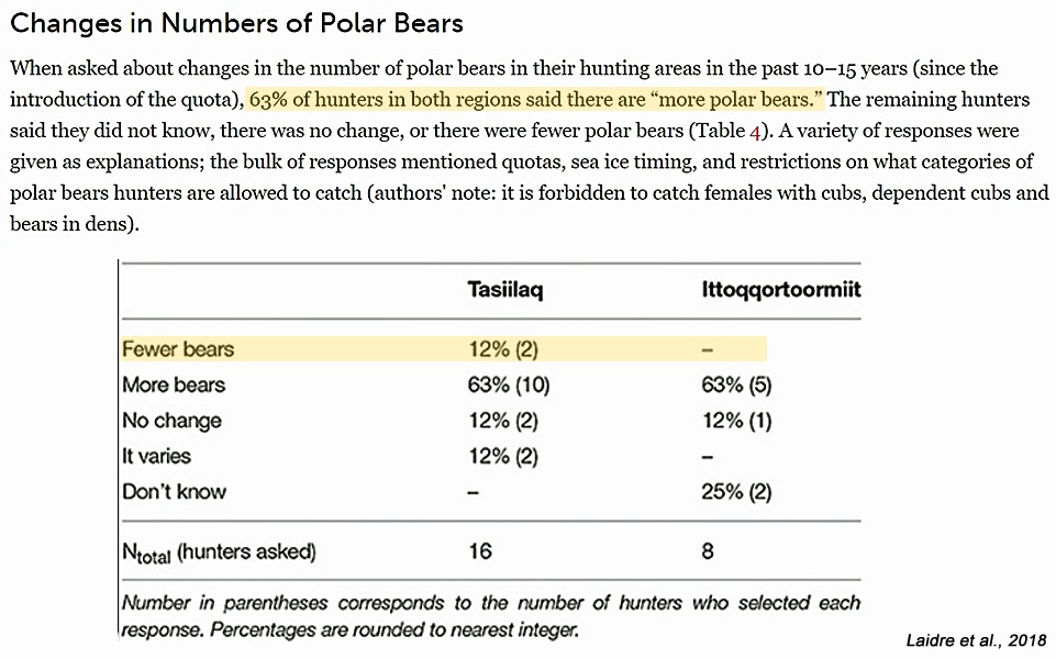
Florko et al., 2018     Decreasing sea ice conditions in western Hudson Bay and an increase in abundance of harbour seals (Phoca vitulina) in the Churchill River … We documented an increase in abundance over the study period; the maximum number of harbour seals observed hauled out at one time was 142 in 2016, compared to a maximum of 32 observed during monitoring activities conducted between 1996 and 2005. In addition, newly born harbour seal pups were observed at the haul-out site during the latter study years, an occurrence not observed from 1996 to 2005. We suggest that an increase in the abundance of harbour seals in Hudson Bay and potentially the entire Arctic may be observed if climate change related reductions in the duration of ice cover continue.

Feng et al., 2018     [E]nvironmental conditions in years with less ice cover were more favorable for C. glacialis development than those with more ice cover. The highest success rate (85.3%) occurred in 2012, coincident with the year of the lowest sea ice extent among the 35-year study period. Transition-zone annual mean temperature was negatively correlated with September-mean sea ice extent (r = −.92, p < .01), as was food availability (r = −.96, p < .01). Annual mean temperature and food for the transition-zone individuals also showed significant upward trends although temperature appeared to have much higher variability than food.  In the Chukchi Sea, significant increases in the biomass and abundance of zooplankton (particularly C. glacialis) were found in recent warm years as compared to the earlier cold years (Ershova et al., 2015). The strong positive correlation between mean developmental stage of C. glacialis and sea surface temperature from that study agreed with our modeling results, both suggesting that warmer temperatures sped up C. glacialis cohort developmental process.

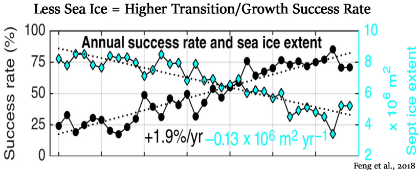
Yang et al., 2018     Adélie penguin populations as inferred from […] southern Cape Bird declined slightly from ∼1450 to ∼1600 AD, began to rise afterward and reached their highest level in ∼1700 AD, then declined with fluctuations to the lowest levels through ∼1900 AD. For the past 100 yr, Adélie penguin populations experienced a sharp rise and drop. Monitoring data have shown that Adélie penguins at Cape Bird had an increasing trend in the 1970s, likely linked with changes in sea-ice extent and polynya size, but also with variation in competition with minke whales (Ainley et al., 2005; Wilson et al., 2001). Our study suggests that the penguin populations increased in the 1960s as well, consistent with their research. … Over the past 500 yr at Cape Bird, Adélie penguin populations increased during the cold period (∼1600–1825 AD), which is inconsistent with the general pattern in other studies, for example, penguin populations increased when climate became warmer, and vice versa (Emslie et al., 2007; Huang et al., 2009; Sun et al., 2000). 

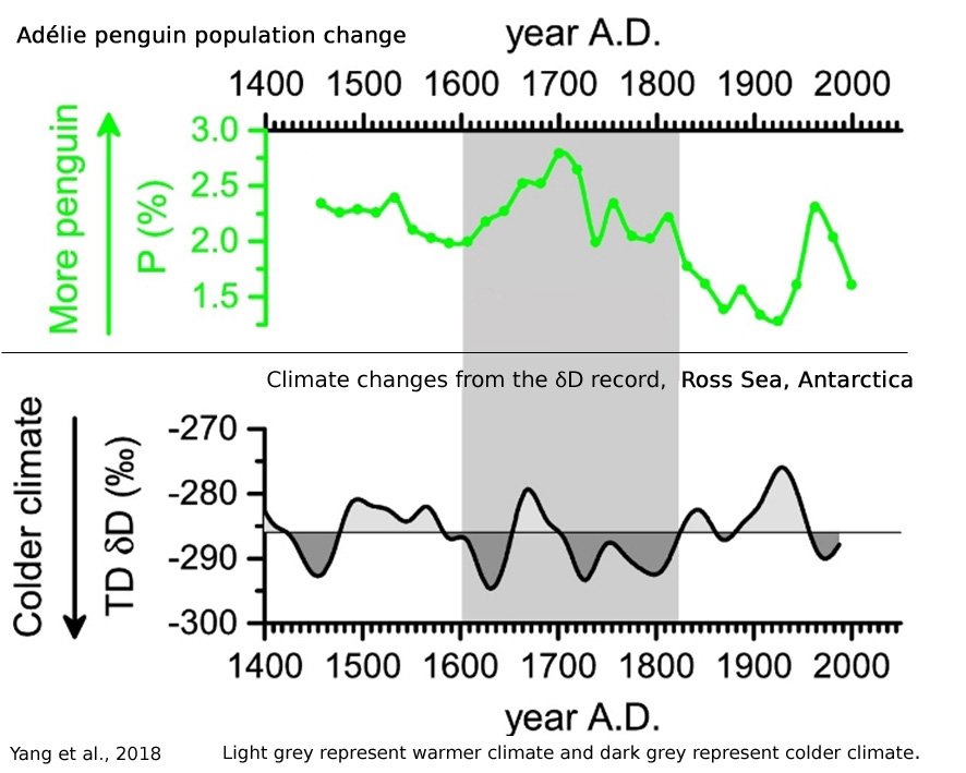
Foley et al., 2018     While dramatic increases in populations of King Penguins (Aptenodytes patagonicus) have been documented throughout their range, population changes on the island of South Georgia have not been assessed. We reconstructed time series of population size for six major colonies across South Georgia using historical data stretching back to 1883 and new population estimates derived from direct on-the-ground censuses and oblique, high-resolution digital photographs. We find evidence for a significant increase in the population of King Penguins at all colonies examined over the 124 years of available survey data.

Askeyev et al., 2018     The aim of this study was to investigate the impact of climate change on the population dynamics of ten species of Passeriformes in the Tartarstan Republic, Russia. Ravkin’s transect method was used to census fixed randomly selected plots spread over a large geographic area at least once every month for the past 26 years. Observers remained the same over the whole period. The abundance of nine species in the first half of the winter and four species in the second half of the winter showed significant increases during the study period. Unlike studies from countries in Western Europe, there were no significant decreases in these species. Significant changes in winter conditions, as well as during the breeding season, and an overall increase in annual temperatures are likely reasons for a significant increase in the number of birds in winter. Greater winter survival, an increase in the survival rate of fledglings and juveniles during the summer, and later onset of winter, are very important determinants of the winter population. Our findings show that numbers of birds in late winter are related to the severity of winter conditions. Our data do not support conclusions that the populations of forest bird species have decreased due to climate change.

Global Warming Saves Lives. Cold Kills.

Fu et al., 2018     We applied distributed-lag nonlinear models with case-crossover models to assess the effects of heat and cold on all medical causes of death for all ages from birth (n = 411,613) as well as on stroke (n = 19,753), ischaemic heart disease (IHD) (n = 40,003), and respiratory diseases (n= 23,595) among adults aged 30–69. We calculated the attributable risk fractions by mortality cause for extremely cold (0.4 to 13.8°C), moderately cold (13.8°C to cause-specific minimum mortality temperatures), moderately hot (cause-specific minimum mortality temperatures to 34.2°C), and extremely hot temperatures (34.2 to 39.7°C). We further calculated the temperature-attributable deaths using the United Nations’ death estimates for India in 2015. Mortality from all medical causes, stroke, and respiratory diseases showed excess risks at moderately cold temperature and hot temperature. For all examined causes, moderately cold temperature was estimated to have higher attributable risks (6.3% [95% empirical confidence interval (eCI) 1.1 to 11.1] for all medical deaths, 27.2% [11.4 to 40.2] for stroke, 9.7% [3.7 to 15.3] for IHD, and 6.5% [3.5 to 9.2] for respiratory diseases) than extremely cold, moderately hot, and extremely hot temperatures. In 2015, 197,000 (121,000 to 259,000) deaths from stroke, IHD, and respiratory diseases at ages 30–69 years were attributable to moderately cold temperature, which was 12- and 42-fold higher than totals from extremely cold and extremely hot temperature, respectively. The main limitation of this study was the coarse spatial resolution of the temperature data, which may mask microclimate effects. … We demonstrate that cold temperatures contributed to higher attributable risks of mortality than hot temperatures in India during 2001–2013, consistent with previous findings based on nonlinear temperature–mortality associations drawn from mostly high-income countries [2]. These previous findings reported an overall attributable risk of 7.29% (eCI 7.02 to 7.49) for cold temperature and 0.42% (0.39 to 0.44) for hot temperature, which are similar to our results for all ages (Table C in S1 Appendix). Among countries, our results are most comparable to those of Australia.

Vicedo-Cabrera et al., 2018     Table 1 summarizes the mortality and temperature data from the 305 locations distributed in 10 countries included in the study [during 1985-2009] (see also Table S2 in the Appendix). The data included nearly 75 million deaths, and countries contributed an average of 20.5 years to the time series data, ranging from 14 years (Brazil) to 27 years (Japan).   Heat-related AFs decreased in all countries (ranging from 0.45–1.66% to 0.15–0.93%, in the first and last 5-year periods, respectively) except in Australia, Ireland and UK. Different patterns were found for cold (where AFs ranged from 5.57–15.43% to 2.16–8.91%), showing either decreasing (Brazil, Japan, Spain, Australia and Ireland), increasing (USA), or stable trends (Canada, South Korea and UK). Heat-AF trends were mostly driven by changes in exposure-response associations due to modified susceptibility to temperature, whereas no clear patterns were observed for cold. … Cold temperatures exhibit larger attributable mortality (above 5%) compared to heat (around or below 1%) in all countries.  Cold-mortality impacts persisted throughout the study periods in most of the countries, although following different temporal patterns (Fig. S4).  Canada, Japan, Spain, Switzerland, South Korea and the USA show a decreasing trend in heat-attributable AFs, from 0.45–1.66% in the first 5-year sub-period to 0.15–0.93% in the last 5-year sub-period. Heat impacts remained stable in UK and Brazil at around 0.2–0.4% and 0.6–0.7%, respectively, whereas it increased in Australia from 0.05% to 0.67%.

Oudin Åström et al., 2018     Projections of temperature-related mortality rely upon exposure-response relationships using recent data. Analyzing long historical data and trends may extend knowledge of past and present impacts that may provide additional insight and improve future scenarios. We collected daily mean temperatures and daily all-cause mortality for the period 1901–2013 for Stockholm County, Sweden, and calculated the total attributable fraction of mortality due to non-optimal temperatures and quantified the contribution of cold and heat. Total mortality attributable to non-optimal temperatures varied between periods and cold consistently had a larger impact on mortality than heat. Cold-related attributable fraction (AF) remained stable over time whereas heat-related AF decreased. AF on cold days remained stable over time, which may indicate that mortality during colder months may not decline as temperatures increase in the future. More research is needed to enhance estimates of burdens related to cold and heat in the future.

Lee et al., 2018     This study investigated the change in risks of mortality from heat waves and cold spells over time, and estimated the temporal changes in mortality burden attributed to heat waves and cold spells in Korea and Japan. We collected time-series data covering mortality and weather variables from 53 communities in the two countries from 1992 to 2015. Two-stage time-series regression with a time-varying distributed lag model and meta-analysis was used to assess the impacts of heat waves and cold spells by period (1990s, 2000s, and 2010s). In total population, the risks of heat waves have decreased over time; however their mortality burden increased in the 2010s compared to the 2000s with increasing frequency. On the other hand, the risk and health burden of cold spells have increased over the decades.

Shaposhnikov and Revich, 2018     The impacts of increasing year-round temperatures on mortality from all non-accidental, all cardiovascular, and all non-cardiovascular causes were examined in the city of Akchangelsk in Russian North, where the climate change signal is expected to be stronger than the global average. Projections of future daily temperatures were made for IPCC B2, A1B, and A2 greenhouse gas emission scenarios using regional downscaling of the selected ensemble of 16 general circulation models. The distributed lag nonlinear models were used to estimate 30-day cumulative risks of the exposure to heat and cold. The projected changes in annual fractions of deaths attributed to nonoptimal temperatures are negative and not significant at 95% confidence level for all categories of mortality and emission pathways included in the study. The benefits of reduced cold-related mortality will most likely outweigh the negative impacts of higher heat-related mortality during the projection period 2045–2056. However, this situation may be reversed in the longer run.

Pascal et al., 2018     We investigated the lag structure of the mortality response to cold and warm temperatures in 18 French cities between 2000 and 2010. … The fraction of mortality attributable to cold and heat was estimated with reference to the minimum mortality temperature. … Results: Between 2000 and 2010, 3.9% [CI 95% 3.2:4.6] of the total mortality was attributed to cold, and 1.2% [1.1:1.2] to heat.

Scovronick et al., 2018     We conducted a time-series analysis using daily temperature data and a national dataset of all 8.8 million recorded deaths in South Africa between 1997 and 2013. Mortality and temperature data were linked at the district municipality level and relationships were estimated with a distributed lag non-linear model with 21 days of lag, and pooled in a multivariate meta-analysis.  We found an association between daily maximum temperature and mortality. Total attributable mortality was 3.4%, mostly from cold (3.0%) rather than heat (0.4%).

Longden et al., 2018     The importance of assessing the nature of the temperature-mortality relationship using different techniques and data from a range of climatic regions is important as previous studies, which includes Guo et al. (2016) and Gasparrini et al. (2017), have found net benefits from climate change that are associated with decreased cold temperature-related deaths in regions that are subject to extremely warm temperatures.

Bai et al., 2018     Between 1996 and 2013, we identified 1.4 million hospitalisations from CHD [coronary heart disease] and 355 837 from stroke across Ontario. On cold days with temperature corresponding to the 1st percentile of temperature distribution, we found a 9% increase in daily hospitalisations for CHD (95% CI 1% to 16%), 29% increase for AMI (95% CI 15% to 45%) and 11% increase for stroke (95% CI 1% to 22%) relative to days with an optimal temperature. High temperatures (the 99th percentile) also increased CHD hospitalisations by 6% (95% CI 1% to 11%) relative to the optimal temperature. These estimates translate into 2.49% of CHD [coronary heart disease] hospitalisations attributable to cold and 1.20% from heat. Additionally, 1.71% of stroke hospitalisations were attributable to cold.

Warming, Acidification Not Harming Oceanic Biosphere

Thor et al., 2018     Uptake of anthropogenic CO2 is changing the chemistry of the global ocean [1]. When entering the sea, CO2 reacts with water to form carbonic acid, and this ocean acidification (OA) has lowered the global ocean mean surface pH from 8.13 during the pre-industrial age to the present day 8.05. This trend is predicted to continue and current models estimate a further decrease of up to 0.4 pH units by the year 2100. [A pH unit change of 0.08 in 250 years, 0.0003 per year, vs. a projected pH unit change of 0.4 over the next 85 years.] … We incubated females at present day conditions (pHT 8.0) and year 2100 extreme conditions (pHT 7.5) during oogenesis and subsequently reciprocally transplanted laid eggs between these two conditions. Statistical tests showed no effects of maternal or direct exposure to OA [ocean acidification] at this level [7.5 pHT].

McCulloch et al., 2018     For example, over seasonal time-scales Porites corals from the Great Barrier Reef (GBR) have a large range in pHcf of ~8.3 to ~8.5, significantly greater (~×2 to ~×3) than that of reef-water (pHT ~8.01 to ~8.08), and an order of magnitude greater than that expected from ‘static’ laboratory experiments. Strong physiological controls, but of a different character, are found in corals grown in a Free Ocean Carbon Enrichment Experiment (FOCE) conducted in situ within the Heron Island lagoon (GBR). These corals exhibit near constant pHcf values regardless of external changes in temperature and seawater pH. This pattern of strong physiologically controlled ‘pH-homeostasis’, with elevated but constant pHcf has been found despite large natural seasonal variations in the pH (±0.15 pH units) of the lagoon waters, as well as the even larger super-imposed decreases in seawater pH (~0.25 pH units) designed to simulate year 2100 conditions. In natural reef environments we thus find that the processes influencing the up-regulation of pHcf in symbiont-bearing corals are subject to strong physiological controls, behaviour that is not well simulated in the current generation of aquaria-based experiments with fixed seawater pH and temperature.

Sswat et al., 2018     Over a period of 32 days, larval survival, growth in size and weight, and instantaneous growth rate were assessed in a crossed experimental design of two temperatures (10°C and 12°C) with two CO₂ levels (400 μatm and 900 μatm CO₂) at food levels mimicking natural levels using natural prey. Elevated temperature alone led to increased swimming activity, as well as decreased survival and instantaneous growth rate (G_i). The comparatively high sensitivity to elevated temperature in this study may have been influenced by low food levels offered to the larvae. Larval size, G_i and swimming activity were not affected by CO₂, indicating tolerance of this species to projected “end of the century” CO₂ levels. A synergistic effect of elevated temperature and CO₂ was found for larval weight, where no effect of elevated CO₂ concentrations was detected in the 12°C treatment, but a negative CO₂ effect was found in the 10°C treatment. Contrasting CO₂ effects were found for survival between the two temperatures. Under ambient CO₂ conditions survival was increased at 12°C compared to 10°C.

Hernandez et al., 2018     Decreased pH [ocean “acidification”] had a positive effect on short-term production of the studied species. Algae with tropical affinity increased their production at higher temperatures. Respiration rates were higher at the lower temperature treatments. Future pH and temperature conditions benefit tropical algal species. … The results suggest that biomass and productivity of the more tropical species in coastal ecosystems would be enhanced by future ocean conditions.

Gao et al., 2018     Ulva is increasingly viewed as a food source in the world. Here, Ulva rigida was cultured at two levels of temperature (14, 18 °C), pH (7.95, 7.55, corresponding to low and high pCO2), and nitrate conditions (6 μmol L−1, 150 μmol L−1), to investigate the effects of ocean warming, acidification, and eutrophication on food quality of Ulva species. High temperature increased the content of each amino acid. High nitrate increased the content of all amino acids except aspartic acid and cysteine. High temperature, pCO2, and nitrate also increased the content of most fatty acids. The combination of high temperature, pCO2, and nitrate increased the swelling capacity, water holding capacity, and oil holding capacity by 15.60%, 7.88%, and 16.32% respectively, compared to the control. It seems that the future ocean environment would enhance the production of amino acid and fatty acid as well as the functional properties of Ulva species.

Huang et al., 2018     When air CO₂ was elevated to 750 ppm, the inorganic carbon contents in media increased, thereby stimulating algal reproduction and photosynthesis. Moreover, the volumes of unicells and two‐celled colonies were enlarged under elevated CO₂ conditions. These physiological changes satisfied the material and energy demands for the formation of larger colonies. 

Schunter et al., 2018     Importantly, we find that altered gene expression for the majority of within-generation responses returns to baseline levels following parental exposure to elevated CO2 conditions. Our results show that both parental variation in tolerance and cross-generation exposure to elevated CO2 are crucial factors in determining the response of reef fish to changing ocean chemistry.

Baumann et al., 2018     Starvation rates in larval and juvenile Atlantic silversides (Menidia menidia) are unaffected by high CO2 conditions …  Contrary to expectation, we found that starvation rates were largely independent of the CO2 environment in this fish species. The one exception occurred at the lowest temperature and most extreme CO2 treatment, which resulted in slower not faster starvation in newly hatched larvae at high compared to ambient CO2 treatments.

Cross et al., 2018    Although information from long-term laboratory experiments is vital to reveal sensitivities of marine organisms, even they can still only predict responses from exposures of relatively short durations, of months or even a few years, to environmentally unrealistic conditions (Andersson et al., 2015; Riebesell & Gattuso, 2015). …  Here, we present data from a novel approach that assesses responses over a centennial timescale showing remarkable resilience to change in a species predicted to be vulnerable. Utilising museum collections allows the assessment of how organisms have coped with past environmental change. It also pro-vides a historical reference for future climate change responses. We evaluated a unique specimen collection of a single species of brachiopod (Calloria inconspicua) collected every decade from 1900 to 2014 from one sampling site. The majority of brachiopod shell characteristics remained unchanged over the past century. One response, however, appears to reinforce their shell by constructing narrower punctae (shell perforations) and laying down more shell. This study indicates one of the most calcium-carbonate-dependent species globally to be highly resilient to environmental change over the last 120 years and provides a new insight for how similar species might react and possibly adapt to future change.

Liu et al., 2018     The chlorophyll a (Chl a), carotenoid (Car), and phycobiliprotein (PB) contents responded significantly to increased temperature under normal CO2 and high CO2 concentrations. However, CO2 enrichment in the culture had no significant impact on Chl a and Car but decreased the PB contents in G. lemaneiformis. The growth rates of G. lemaneiformis were significantly improved by increasing temperature, especially under concurrent increasing CO2 levels. Additionally, short-term exposure to high temperature stimulated the irradiance-saturated maximum photosynthetic rate (P max), and this stimulation was preserved with exposure to the high temperature in long-term incubations, with such stimulation being much more pronounced under normal CO2 concentrations than high CO2 concentrations. Results suggest that increased temperature exerted more pronounced effects on the growth and photosynthesis of G. lemaneiformis than increased CO2 concentrations did. We proposed that the sea cultivation of G. lemaneiformis would benefit from the ongoing climate change (increasing atmospheric CO2 concentrations and sea surface temperatures) through enhanced growth and carbon sequestration.

Henkes et al., 2018     [T]ropical temperatures during the icehouse climate of the Carboniferous period were broadly similar to present (∼25–30°C), and suggests that benthic metazoans were able to thrive at temperatures of 35–40°C during intervals of the early and possibly the latest Paleozoic when CO2 levels were likely 5–10× higher than present-day values. … This Paleozoic clumped isotope record also suggests that marine animals thrived in water temperatures of 35–40°C for long intervals of time and across widespread regions of the oceans. Compelling evidence for sea surface temperatures of 30–35°C has also been presented for other warm intervals in Earth history, including the early Ordovician (summarized above), early to middle Triassic (Sun et al. 2012), and middle Eocene (Pearson et al., 2007).

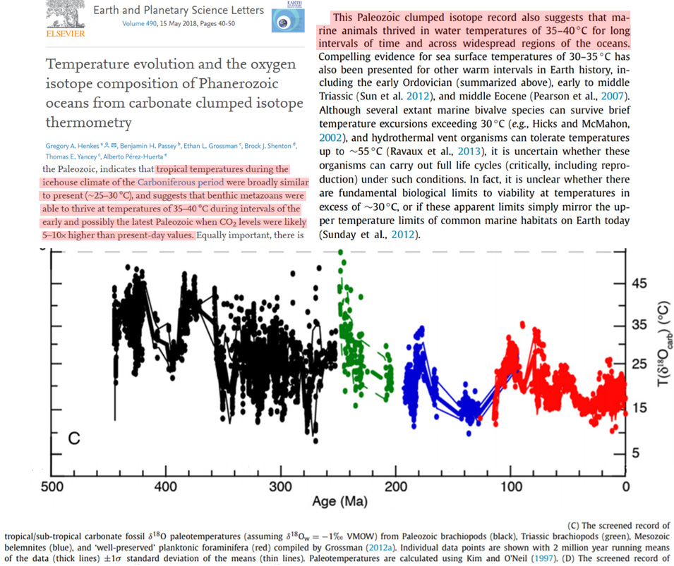
Coral Bleaching Is A Natural, Non-Anthropogenic Phenomenon

Kamenose and Hennige, 2018     Reconstructed bleaching was evident through the entire available record from 1575 to 2001. To determine any GBR-wide bleaching patterns, corals were pooled from all regions in the GBR spanning 15.13 to 22.23°S. Quantitative assessments of bleaching were conducted between 1620 and 2001 for frequency and 1640–2001 for prevalence. Outside of these periods, while we have documented historic bleaching, it is possible that the number of cores available drove the patterns observed. … Reconstructed bleaching frequency demonstrated three trends; (1) frequency increased from 1620 to 1753 ± 31 (years) reaching up to 6 years of each decade showing evidence of bleaching in at least 20% of coral cores. (2) Bleaching frequency decreased to 1820 ± 31 when only 1 year of every decade had evidence of bleaching in at least 20% of coral cores. (3) Bleaching frequency increased again from 1820 ± 31 to 2001. The 1890 and 1750 decades were notable for unusually high bleaching frequencies. In contrast to bleaching frequency, bleaching prevalence only demonstrated two trends; (1) a negative trend from 1640 – 1774 ± 78, with prevalence falling from 41 to 21%. 2) An increase in bleaching prevalence from 21% in 1774 ± 78 to 31 % in 2001.

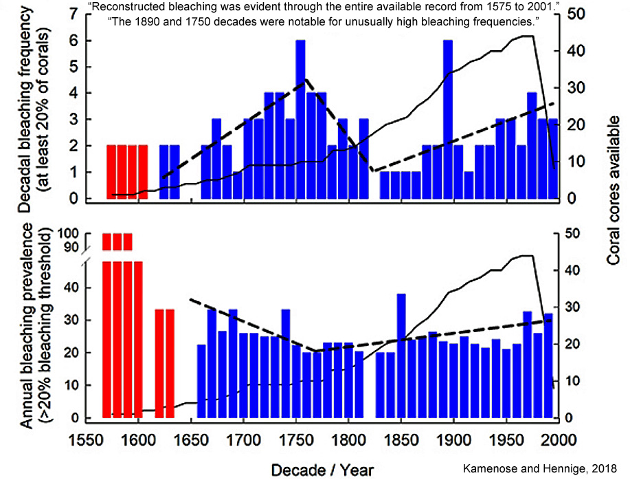
Xu et al., 2018     This study provides evidence that thermal coral bleaching events have occurred in the warmer mid-Holocene (where maximum monthly summer SST was 2 °C higher than at present) in Hainan island.  … We carried out this pilot study to explore the responses of corals to abnormally warm conditions in prehistoric periods. Four massive Porites coral fossils that died 3800 – 4200 years ago were collected from the Wenchang fringing reef, Hainan Island, NSCS. The reconstructed SST just prior to the mortality surfaces and growth discontinuities were higher than the [modern] maximum summer SSTs in the NSCS [Northern South China Sea]. This indicated that the corals’ deaths and interruptions in growth – which were observed to be in summer – were accompanied by an anomalously high SST [sea surface temperature]. Enhanced Δδ18O suggested increased evaporation and high-SSS conditions, attributable to warm sea surface temperatures. A significant negative shift in δ13C just prior to mortality surfaces and growth discontinuities indicated a reduced photosynthetic intensity of symbiotic zooxanthellae. Together, this evidence for increased SST and SSS and decreased photosynthetic intensity strongly suggest that the growth hiatuses and coral deaths observed were the results of severe coral bleaching.This in turn indicates that coral bleaching events under high SST conditions have already occurred in the mid-Holocene and are by no means a new ecological phenomenon of current global warming.

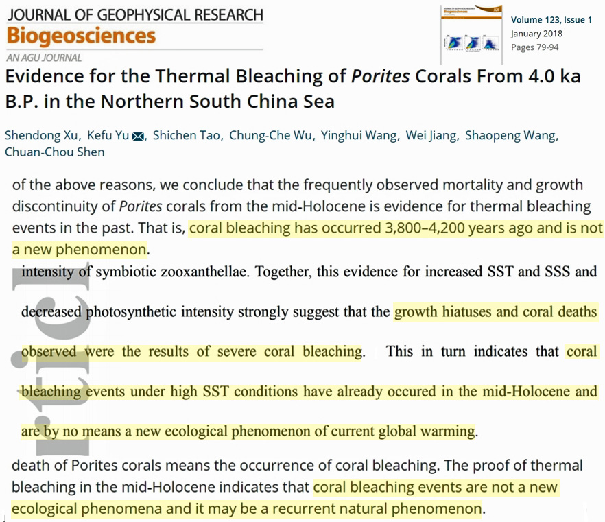
No Increasing Trends In Intense Hurricanes, Storms

Truchelut and Staeling, 2018     The extremely active 2017 Atlantic hurricane season concluded an extended period of quiescent continental United States tropical cyclone landfall activity that began in 2006, commonly referred to as the landfall drought. We introduce an extended climatology of U.S. tropical cyclone activity based on accumulated cyclone energy (ACE) and use this data set to investigate variability and trends in landfall activity. The [hurricane landfall] drought years between 2006 and 2016 recorded an average value of total annual ACE [accumulated cyclone energy] over the U.S. that was less than 60% of the 1900–2017 average. Scaling this landfall activity metric by basin-wide activity reveals a statistically significant downward trend since 1950, with the percentage of total Atlantic ACE expended over the continental U.S. at a series minimum during the recent drought period.

Klotzbach et al., 2018     Continental United States (CONUS) hurricane-related inflation-adjusted damage has increased significantly since 1900. However, since 1900 neither observed CONUS [Continental United States] landfalling hurricane frequency nor intensity show significant trends, including the devastating 2017 season.

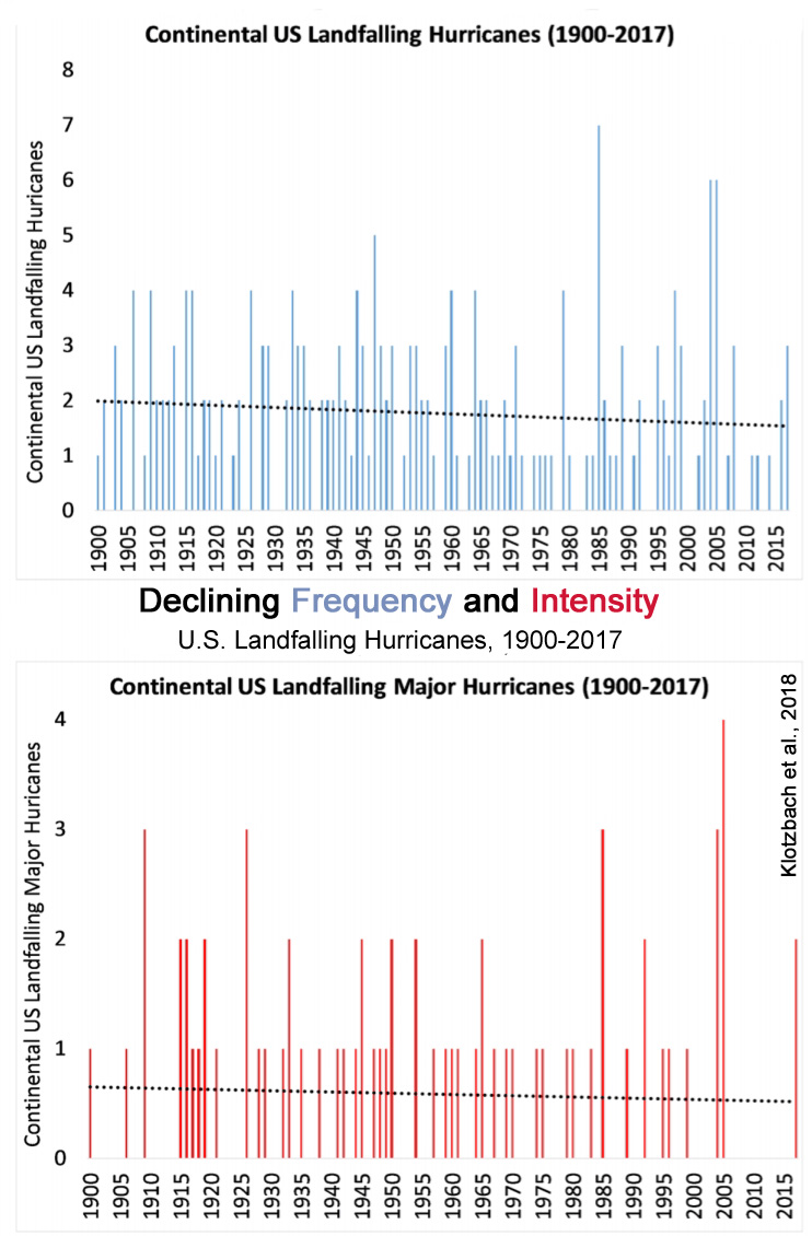
Zhang et al., 2018     Over the 1997–2014 period, the mean frequency of western North Pacific (WNP) tropical cyclones (TCs) was markedly lower (~18%) than the period 1980–1996. Here we show that these changes were driven by an intensification of the vertical wind shear in the southeastern/eastern WNP tied to the changes in the Walker circulation, which arose primarily in response to the enhanced sea surface temperature (SST) warming in the North Atlantic, while the SST anomalies associated with the negative phase of the Pacific Decadal Oscillation in the tropical Pacific and the anthropogenic forcing play only secondary roles.

Zhao et al., 2018     A vigorous debate has currently focused on the relationship between increasing TC [tropical cyclone] activity and increasing SST [sea surface temperatures] (Knutson et al. 2010). … [O]ver the WNP [Western North Pacific] basin, a significant decrease of TCF [tropical cyclone frequency] has been observed since 1998 (Liu and Chan 2013; Lin and Chan 2015; Zhao and Wang 2016). Global TCF [tropical cyclone frequency] has showed a similar reduction since the late 1990s (Maue 2011). Change of TCF over the past few decades does not appear to be consistent with changes in local SST. Observational analyses further pointed out that there is no significant correlation between the TCF [tropical cyclone frequency] and local SST [sea surface temperatures] over the WNP  [Western North Pacific] basin (Chan 2006; Yeh et al. 2010).

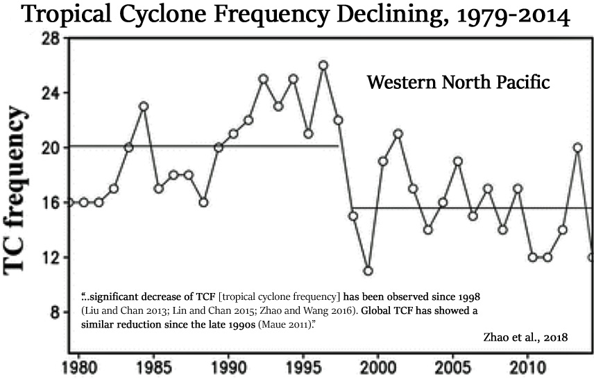
Aryal et al., 2018     TCs [tropical cyclones] contribute to ∼20–30% of AMs and POTs over Florida and coastal areas of the eastern United States, and the contribution decreases as we move inland. … The record length ranges from 50 to 153 years and a large number of 121 stations have discharge measurements from 1950 onwards. … We do not detect statistically significant trends in the magnitude or frequency of TC [tropical cyclone] floods.

Zou et al., 2018     The Tibetan Plateau (TP), one of the world’s most sensitive areas to climate change, became significantly warmer during recent decades. Since 1960 (1980), storm (hail) days have been decreasing by 6.2%/decade (18.3%/decade) in the region. … Based on 53‐year continuous weather records at 48 TP stations and reanalysis data, we show here for the first time that the consistent decline of storm days is strongly related to a drier midtroposphere since 1960. Further analysis demonstrated that fewer hail days are driven by an elevation of the melting level (thermodynamically) and a weaker wind shear (dynamically) in a warming climate.These results imply that less storm and hail may occur over TP when climate warms.

Hu et al., 2018     Tropical cyclone (TC) genesis frequency in the western North Pacific (WNP) during 1960–2014 shows a step-by-step decrease on interdecadal timescale, in accordance to the phase of the Interdecadal Pacific Oscillation (IPO). The environmental parameters responsible for the interdecadal change of TC genesis frequency were investigated. It was found that vertical wind shear especially the zonal wind shear plays a critical role, while other parameters such as sea surface temperature (SST), vertical velocity, divergence, humidity and maximum potential intensity cannot explain the step-by-step decrease of TC genesis frequency. … A further diagnosis shows that the interdecadal change of vertical wind shear is caused by SST and associated rainfall pattern changes across the Indo-Pacific Ocean. A stronger warming in the Indian Ocean/western Pacific from 1960–1976 to 1977–1998 led to enhanced convection over the Maritime Continent and thus strengthened vertical shear over the key TC genesis region in the WNP. A La Nina-like SST pattern change from 1977–1998 to 1999–2014 led to a strengthened Walker circulation in the tropical Pacific, which further enhanced the vertical shear and decreased TC genesis frequency in the WNP.

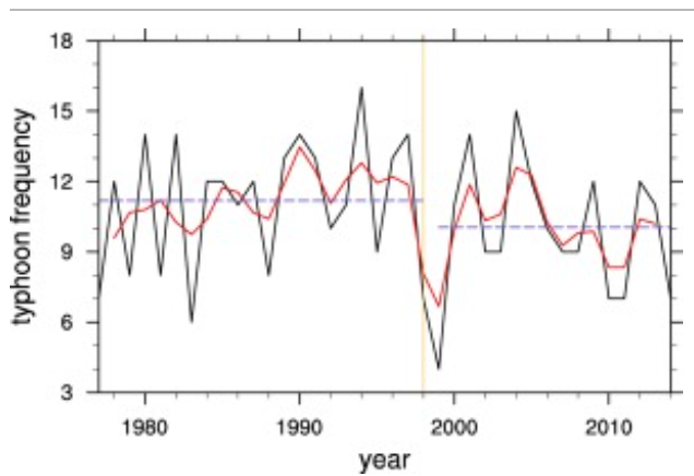
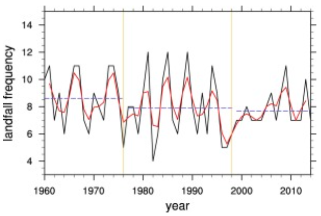
Weinkle et al., 2018     This analysis provides a major update to the leading dataset on normalized US hurricane losses in the continental United States from 1900 to 2017. Over this period, 197 hurricanes resulted in 206 landfalls with about US$2 trillion in normalized (2018) damage, or just under US$17 billion annually. Consistent with observed trends in the frequency and intensity of hurricane landfalls along the continental United States since 1900, the updated normalized loss estimates also show no trend. A more detailed comparison of trends in hurricanes and normalized losses over various periods in the twentieth century to 2017 demonstrates a very high degree of consistency.

No Increasing Trend In Drought/Flood Frequency, Severity 

Guo et al., 2018   In drought-prone regions like Central Asia, drought monitoring studies are paramount to provide valuable information for drought risk mitigation. In this paper, the spatiotemporal drought characteristics in Central Asia are analyzed from 1966 to 2015 using the Climatic Research Unit (CRU) dataset. Central Asia showed an overall wetting trend with a switch to drying trend since 2003.

Mangini et al., 2018     The main objective of this paper is to detect the evidence of statistically significant flood trends across Europe using a high spatial resolution dataset. … Anticipated changes in flood frequency and magnitude due to enhanced greenhouse forcing are not generally evident at this time over large portions of the United States for several different measures of flood flows. … Thus, similarly to the main findings of Archfield et al. (2016) for the US, the picture of flood change in Europe is strongly heterogeneous and no general statements about uniform trends across the entire continent can be made.

Zheng et al., 2018     For the extreme drought and flood events in total, more frequent of them occurred in the 1770s and 1790s, 1870s–1880s, 1900s–1920s and 1960s, among which the 1790s witnessed the highest frequency of extreme drought and flood events totally.

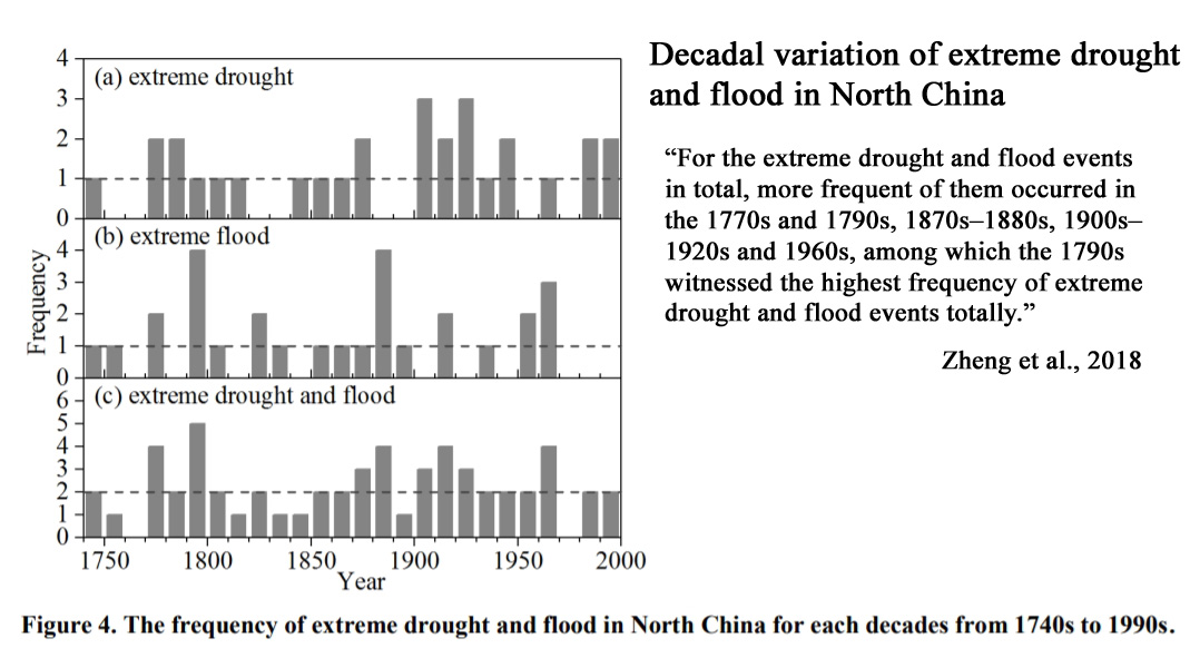
Schedel, Jr. and Schedel, 2018    Flood events on the U.S. East Coast are not more severe or frequent than in the past. However, because of sea-level rise, these events are starting from a higher baseline height. Thus, the same severity of a flood event today reaches a greater absolute height than an identical flood would have reached 50 or 100 years ago. Based on current data, the good news is that the apparent worsening of flood events is due to a single, primary cause: sea level rise. Flood events are not getting stronger or occurring more frequently than in the past. They are instead starting from a higher point, allowing them to reach higher levels more often. The bad news is that sea-level rise will be a fact of life for many years into the future. Communities need to start now to make informed plans and decisions about how best to adapt.

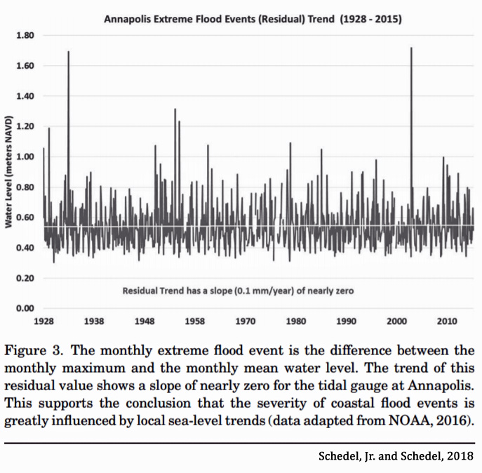
Valdés-Manzanilla, 2018     This study presents a chronology of historical and measured flood events in the Papaloapan River basin of Mexico during 450 years. Twenty-eight historical floods were recorded during the period 1550–1948 [7 per century] on this river and one flood event (1969) in the instrumental era (1949–2000) [2 per century], of which 14 were extraordinary floods and only 15 were catastrophic ones. There were several flood-rich decades during 1860–1870, 1880–1890, 1920–1930 and 1940–1950. Wavelet analysis found a significant flooding periodicity of 58 years. The wavelet coherence analysis found that flooding had an in-phase relationship with the Atlantic Multidecadal Oscillation and also with the Pacific Decadal Oscillation. Logistic regression corroborated that there exists a positive relationship between floods events and these two natural climatic oscillations. The logistic regression model predicted correctly 92% of flood events.

Ault and George, 2018     Several lines of evidence now suggest that the western US was hit by multiple megadroughts within the past thousand years. … Paleoclimate research has shown that long intervals of unbroken drought are not just a plot device used by mythmakers but rather a normal feature of climate in many parts of the world. Although the westward expansion of the US coincided with a climatic interval that has been, by and large, free of megadrought, the American West could soon slip into a decades-long drought, even without any unusual climate forcing. In physical climatology, there are two schools of thought regarding how megadroughts occur. The first posits that long-lived droughts are a consequence of external climate forcing: volcanic eruptions, fluctuations in the Sun’s output, small changes in Earth’s orbit, and other factors that influence our planet’s climate but are not affected by it. …  A second school of thought holds that the flurry of megadroughts could have been a mere coincidence. … The paleoclimate community still isn’t sure which explanation is correct. But the answer bears directly on our ability to gauge the odds of future megadroughts. If the medieval megadroughts that plagued the western US were caused by increased solar irradiance, that could imply that the region is particularly sensitive to changes in radiative forcing and temperature. Present-day climate change, marked by increasing surface temperatures and increased downward IR radiation, would therefore be expected to profoundly influence regional megadrought risks. But if megadroughts don’t require any particular external forcing, the risk of recurrence will depend strongly on the natural variations of the climate system.

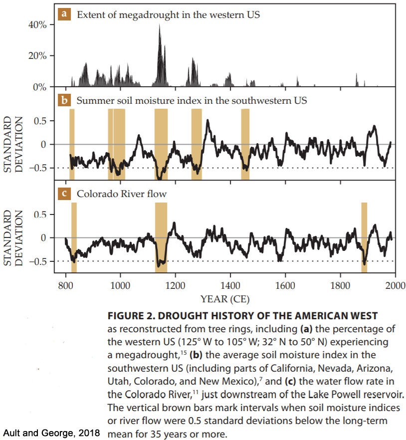
Zhao et al., 2018

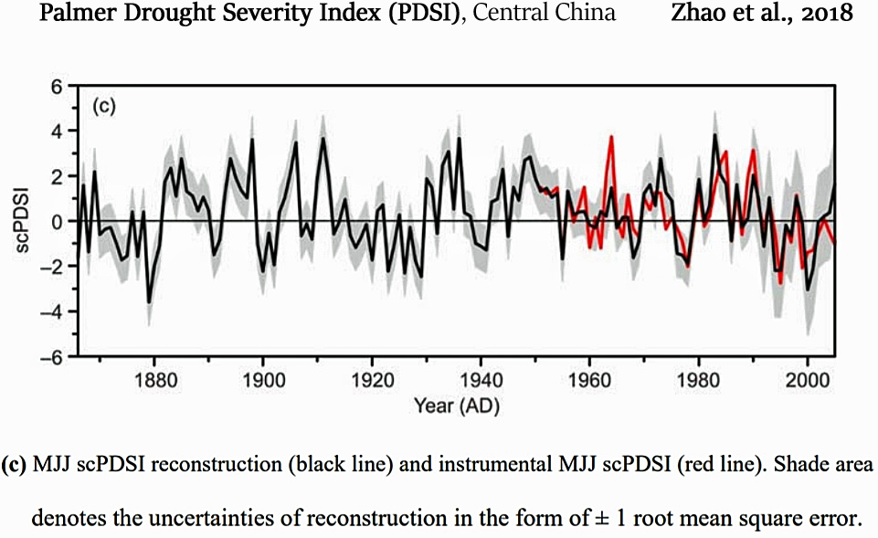
Natural CO2 Emissions A Net Source, Not A Net Sink

Biswas et al., 2018     The era of global warming and increased emission of greenhouse gases can be marked by the beginning of the industrial age. It is also true that under several conditions, natural ecosystems can be equally responsible for CO2 emission like any other anthropogenic activities which continuously release heat-trapping gases in the process of development. … East Kolkata Wetland (EKW) is an urban or peri-urban wetland located on the outskirts of the Kolkata City which performs multi-facet activities, carbon sink being one of them. The raw waste from the city is naturally treated in this wetland system, however, the aquaculture ponds situated in these wetlands which make use of this waste water for fishery is rarely studied. The present study aims to see whether the aquaculture ponds of EKW complex are acting as a source or a sink. Airwater carbon dioxide (CO2) flux was estimated for three consecutive seasons in a year and it was found that the system is acting as a CO2 source in all the three seasons.

Wang et al., 2018     We conducted a free‐water mass balance‐based study to address the rate of metabolism and net carbon exchange for the tidal wetland and estuarine portion of the coastal ocean and the uncertainties associated with this approach were assessed. We measured open water diurnal O2 and dissolved inorganic carbon (DIC) dynamics seasonally in a salt marsh‐estuary in Georgia, U.S.A. with a focus on the marsh‐estuary linkage associated with tidal flooding. We observed that the overall estuarine system was a net source of CO2 to the atmosphere and coastal ocean and a net sink for oceanic and atmospheric O2.

Li et al., 2018     Our calculated CO2 areal fluxes were in the upper-level magnitude of published data, demonstrating the importance of mountainous rivers and streams as a global greenhouse gas source, and urgency for more detailed studies on CO2 degassing, to address a global data gap for these environments. …  Rivers have been widely reported to be supersaturated in carbon dioxide (CO2) with respect to the atmosphere, and are a net source of atmospheric CO2 (Butman and Raymond, 2011; Raymond et al., 2013).

Rosentreter et al., 2018     Although the overall status of mangroves [creeks] is net autotrophic (Alongi, 2002), mangrove sediments and waters have been shown to be a large source of CO2 to the atmosphere due to large organic matter inputs from diverse sources such as the mangrove biomass itself, other terrestrial detritus, nutrients from land, microphytobenthos, phytoplankton and the exchange of organic matter with the open ocean (Lekphet et al., 2005; Borges et al., 2005; Bouillon and Boschker, 2006; Kristensen et al., 2008). … The vast majority of mangrove CO2 gas exchange studies found surrounding waters were supersaturated in CO2 with respect to the atmosphere, hence, a net source of CO2.

Spafford and Risk, 2018     Lakes may function as either sinks or sources of CO₂. … We quantified the net surface flux of CO₂ across a transect of the littoral zone [near shore area] of a small deep oligotrophic lake in eastern Nova Scotia, Canada, and examined potential drivers. The littoral zone [near shore area] was a net source for CO₂, on average emitting 0.171 ± 0.023 μmol CO₂ · m⁻² · s⁻¹, but we did observe significant temporal variation across diel and seasonal periods, as well as with distance from shore.

Global Fire Frequency Declining As CO2 Rises

Earl and Simmonds, 2018     We find that there is a strong statistically significant decline in 2001–2016 active fires globally linked to an increase in net primary productivity observed in northern Africa, along with global agricultural expansion and intensification, which generally reduces fire activity.

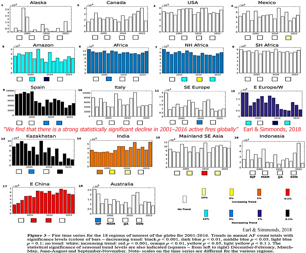
Ward et al., 2018     Globally, fires are a major source of carbon from the terrestrial biosphere to the atmosphere, occurring on a seasonal cycle and with substantial interannual variability. To understand past trends and variability in sources and sinks of terrestrial carbon, we need quantitative estimates of global fire distributions. … Global fire emissions of carbon increase by about 10% between 1700 and 1900, reaching a maximum of 3.4 Pg C yr−1 in the 1910s, followed by a decrease to about 5% below year 1700 levels by 2010. The decrease in emissions from the 1910s to the present day is driven mainly by land use change, with a smaller contribution from increased fire suppression due to increased human population and is largest in Sub‐Saharan Africa and South Asia. Interannual variability of global fire emissions is similar in the present day as in the early historical period, but present‐day wildfires would be more variable in the absence of land use change.

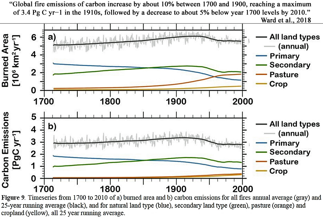
CO2 Changes Lag Temperature Changes By 1000+ Years

Koutavas et al., 2018     The EEP [eastern equatorial Pacific] stack shows persistent covariation with Antarctic temperature on orbital and millennial timescales indicating tight coupling between the two regions. This coupling however cannot be explained solely by CO2 forcing because in at least one important case, the Marine Isotope Stage (MIS) 5e–5d glacial inception, both regions cooled ∼5–6.5 thousand years before CO2 decreased. More likely, their covariation was due to advection of Antarctic climate signals to the EEP by the ocean. … . The discovery that atmospheric CO2 covaries with Antarctic temperature and global ice volume (Lorius et al., 1990; Lüthi et al., 2008; Petit et al., 1999) has propelled CO2 to the forefront as climatic “globalizer”. However, the processes governing CO2 variability are themselves poorly understood, and likely require an oceanic/climatic trigger in the first place (Adkins, 2013; Ferrari et al., 2014; Sigman et al., 2010). Antarctic ice core records are furthermore ambiguous with regard to the causal relationship between CO2 and temperature. Phase relationships show CO2 lagging behind temperature in the obliquity band (Jouzel et al., 2007) and across some major transitions (Caillon et al., 2003; Fischer et al., 1999; Kawamura et al., 2007; WAIS Divide Project Members, 2013), most prominently during the Marine Isotope Stage (MIS) 5e–5d boundary, i.e. the last glacial inception. Antarctic cooling at this time was associated with a major Milankovitch signal, and appears to have transpired almost entirely before the change in CO2 concentration. It remains unclear whether the temperature lead was restricted to Antarctica or was broader.

Uemura et al., 2018     Precise knowledge of the relationship between changes in temperature, atmospheric CO2 and solar insolation is essential to understanding Earth’s climate system. The values of a temperature proxy, the hydrogen isotopic composition (δD), in the Antarctic EDC ice core have varied in parallel with CO2 concentrations over the past 800 thousand years (kyr; r2 = 0.82). However, δD [temperature] apparently leads CO2 variations. For example, during the last termination (TI), the start of Antarctic warming has been estimated to be synchronous with CO2 increase or to lead CO2 increases by 800 ± 600 years on the East Antarctic Plateau. The lead is ca. 2000 years at a West Antarctic site. Over the past 420 kyr, the Vostok ice core shows that the Antarctic δD temperatures lead the CO2 variations by 1.3 ± 1.0 kyr. During the lukewarm interglacials (430–650 kyr BP), Antarctic δD [temperature] leads CO2 by 1900 years, and the correlation between CO2 and δD is weaker (r2 = 0.57), as determined from the EDC core. … Although the mechanisms underlying the coupling and the phase lags remain unclear, the Southern Ocean region, rather than Antarctica, is thought to play the central role in regulating CO2 variations. A box model, for example, estimated a ca. 60% increase in CO2 during TI that is attributable to direct and indirect temperature effects, such as changes in sea ice cover and vertical mixing in the Southern Ocean. On millennial time scales, a multi-proxy study suggests that an antiphased hemispheric temperature response to ocean circulation changes resulted in Antarctic temperatures leading global temperatures and CO2 during TI [the last glacial termination].  … [O]ur data suggest that the lead in Antarctic δD temperatures (i.e. temperature without correcting for source effects) over CO₂ is partly attributable to the effects of the moisture source on δD temperatures over the past 720 kyr in the obliquity band. These results suggest that the importance of moisture source effects for the obliquity signal in δD. Thus, the source effect must be considered in future research about the relationship between Antarctic temperatures and CO₂. … Within the obliquity frequency band, our analyses suggest that temperature variations in Antarctica have led ocean temperatures throughout the past 720 kyr. This phenomenon is most likely explained by the strong influence of local AMI on ΔT_. … During TI [the last glacial termination], CO₂ rose at ~18 kyr BP, which is related to the melting of the Northern Hemisphere ice sheet and the subsequent weakening of the Atlantic meridional overturning circulation (AMOC). Thus, the timing at which CO₂ begins to rise during a termination would be determined by when the Northern Hemisphere ice sheet begins to melt. When eccentricity is small, the summer insolation maxima are small. Thus, if obliquity rises beyond the threshold of melting, a moderate climate forcing could cause warming enough that the southern margin of the North American ice sheet begin to retreat.

Du et al., 2018     During the last deglaciation (19,000–9,000 years ago), atmospheric CO2 increased by about 80 ppm. Understanding the mechanisms responsible for this change is a central theme of palaeoclimatology, relevant for predicting future CO2 transfers in a warming world. Deglacial CO2 rise hypothetically tapped an accumulated deep Pacific carbon reservoir, but the processes remain elusive as they are underconstrained by existing tracers. … The timing of neodymium isotope changes suggests that deglacial acceleration of Pacific abyssal circulation tracked Southern Hemisphere warming, sea-ice retreat and increase of mean ocean temperature. The inferred magnitude of circulation changes is consistent with deep Pacific flushing as a significant, and perhaps dominant, control of the deglacial rise of atmospheric CO2.

Global Losses/Deaths From Weather Disasters Declining

Bouwer and Jonkman, 2018     Global mortality from storm surges is decreasing … Changes in society’s vulnerability to natural hazards are important to understand, as they determine current and future risks, and the need to improve protection. Very large impacts including high numbers of fatalities occur due to single storm surge flood events. Here, we report on impacts of global coastal storm surge events since the year 1900, based on a compilation of events and data on loss of life. We find that over the past, more than eight thousand people are killed and 1.5 million people are affected annually by storm surges. The occurrence of very substantial loss of life (>10 000 persons) from single events has however decreased over time. Moreover, there is a consistent decrease in event mortality, measured by the fraction of exposed people that are killed, for all global regions, except South East Asia.

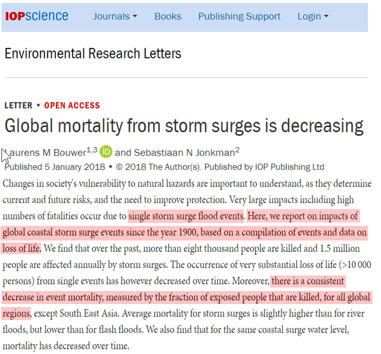
Pielke, 2018     Since 1990 the world has seen a decrease in overall and weather-related disaster losses as a proportion of global GDP. This trend has occurred even as disaster losses have increased in absolute terms. The primary factor driving the overall increase in disaster losses is societal, mainly growth in populations and settlements at risk to the consequences of extreme events (IPCC, 2012).

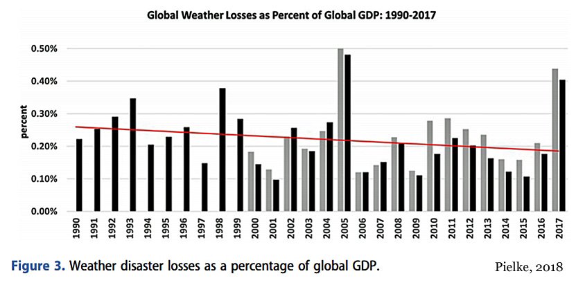
No AGW Changes To Hydrological Cycle Detectable

Nguyen et al., 2018     Little dispute surrounds the observed global temperature changes over the past decades. As a result, there is widespread agreement that a corresponding response in the global hydrologic cycle must exist. However, exactly how such a response manifests remains unsettled. Here we use a unique recently developed long-term satellite-based record to assess changes in precipitation across spatial scales. … Our results show opposing trends at different scales, highlighting the importance of spatial scale in trend analysis. Furthermore, while the increasing global temperature trend is apparent in observations, the same cannot be said for the global precipitation trend according to the high-resolution dataset, PERSIANN-CDR, used in this study. … Figure 2 shows the changes in precipitation volume over oceans and continents during the past 3 decades. As shown in Figs. 2b and 2c, fluctuations are present in the total amount of precipitation that has fallen over land and ocean; however, no significant long-term volumetric change is observed for either case.  … As shown, the warm temperate regions in North America and East Asia, as well as the equatorial regions in Africa, have been experiencing statistically significant negative trends in their mean annual precipitation. On the contrary, arid regions over Africa are observing a positive precipitation trend. In general, warm temperate climate regions have decreasing trends while arid and polar climate regions have increasing trends in precipitation. Africa shows the clearest precipitation trends according to climate zones, where arid regions have a significant increase and the equatorial region has a significant decreasing trend. … Figure 5 shows the precipitation trends over 237 global major basins. Globally, 20 basins have significant increasing trends and 20 basins have significant decreasing trends in precipitation.

The take-home message from our study using the new 33+ years [1983-2015] of high-resolution global precipitation dataset is that there seems not to be any detectable and significant positive trends in the amount of global precipitation due to the now well-established increasing global temperature. While there are regional trends, there is no evidence of increase in precipitation at the global scale in response to the observed global warming.

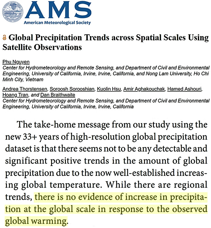
Shi et al., 2018     Here, we average four tree-ring width chronologies from the southeastern Tibetan Plateau (TP) over their common intervals and reconstruct the variability in regional relative humidity (RH) from the previous May to the current March over 1751–2005. In contrast to the summer drying associated with centennial-scale warming and the weakening of the Asian summer monsoon, our RH [relative humidity] reconstruction shows no significant centennial trend from the 1820s through the 2000s.

Silva Junior et al., 2018     The aim of this study was to analyse spatiotemporal trends in rainfall along the Brazilian Legal Amazon between 1998 and 2015. … No evidence of significant rainfall trends (p ≤ 0.05) for annual or monthly (except for September, which showed a significant negative trend) averages was found. … The annual pixel-by-pixel analysis showed that 92.3% of the Brazilian Amazon had no rainfall trend during the period analysed, 4.2% had significant negative trends (p ≤ 0.05), and another 3.5% had significant positive trends (p ≤ 0.05).

Chen et al., 2018     Beyond the general expectation of warming tendency, winter surface air temperature over central Eurasia, parts of North America, and eastern China has exhibited cooling trends during the past two decades, bringing more frequent and severe (even record-breaking) cold waves there [Chen et al., 2017, Liu et al., 2015, McCusker et al., 2016]. Nonetheless, views on the underlying mechanisms for the resurgence of cold extremes, including connection with sea ice losses, Arctic amplification, changes in northern hemisphere circulations, and the relationship with low-frequency sea surface temperature modes of variability (e.g., Pacific Decadal Oscillation—PDO—and Atlantic Multidecadal Oscillation—AMO) still diverge markedly or even are completely opposing [McCusker et al., 2016, Cohen et al., 2014, Sigmond and Fyfe, 2016]. Thus, a better consensus on physical explanations for recent changes in cold extremes calls for more compelling evidence. Exact mechanism understandings would be pivotal for attribution and projection for cold extremes in a warming climate. … The confidence for drought changes over large sections of the world remains low [Field et al., 2012, p. 171]. Greve et al. [2014] and Sheffield et al., [2012] confirmed and further reinforced such low confidence, showing that over much of the global continents, robust dryness tendencies failed to be detected. Thus, the AR5 projections [Stocker et al., 2013, p. 20] that “the contrast in precipitation between wet and dry regions and between wet and dry seasons will increase” (summarized as a “dry gets drier” pattern) does not emerge as a robust feature in observational records, especially after adjusting the definition of dry and wet areas [Greve and Seneviratne, 2015]. … The IPCC AR4 reported that “it is likely that an increase had occurred in intense tropical cyclone activity since 1970 in some regions” [Solomon et al., 2007, p. 239]. But this message was contradicted by the SREX and a World Meteorological Organization assessment [Knutson et al., 2010], which found that, with the exception of the Atlantic Basin, there is low confidence in any observed long-term trend in tropical cyclone activity in other ocean basins, after accounting for past changes in observational system capabilities.

Zhang et al., 2018     Since the surface temperature has changed globally in recent decades, it is reasonable to ask whether PW [precipitable water] has also changed in the past decades. … The global PWs [precipitable water] have been changing in the past 60 years and, to some extent, strongly in recent 10 years. Based on the analysis of the long-term accumulation of radiosonde observations, it is found that PWs at Australian stations present statistically significant decreasing trends in the last 60 years, while PWs at most stations in the US have increasing trends, which is consistent with previous studies. In light of the good performance of the comparisons between two observational data sets, COSMIC data can be a complement to the radiosonde observations due to world-wide measurements. We pay close attention to the global PW [precipitable water] changes in the most recent decade. It is found that PWs [precipitable water] show uptrends over land and downtrends over oceans in the last 10 years, implying the widespread increase of water vapor in the troposphere over land.

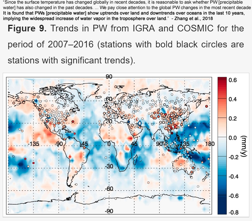
Tabari and Willems, 2018      [C]limate change results are highly model dependent so that even opposite climate change signals may be achieved from different types of climate models. This is mainly due to the fact that climate models with different resolutions and physics provide different representations of surface heterogeneities and mesoscale climatological structures. … We consider a climate change signal to be robust where at least 70% of the models agree on the direction of change. … In contrast to the projected increase in extreme precipitation, there is no robust change in precipitation totals on the global scale. Nevertheless, at the seasonal scale, “wet season becomes wetter, dry season becomes drier” paradigm for precipitation totals has been found in the literature, following a similar physical reasoning explaining the “wet regions get wetter, dry regions get drier”, or the rich-get-richer mechanism. Yet, some researchers believe that “dry gets drier, wet gets wetter” paradigm has been overestimated and a large part of the land area experience an opposite paradigm. Such contradicting results are likely connected to the type of data/model used and the transition of humid regions towards drier conditions or vice versa under future climate conditions.

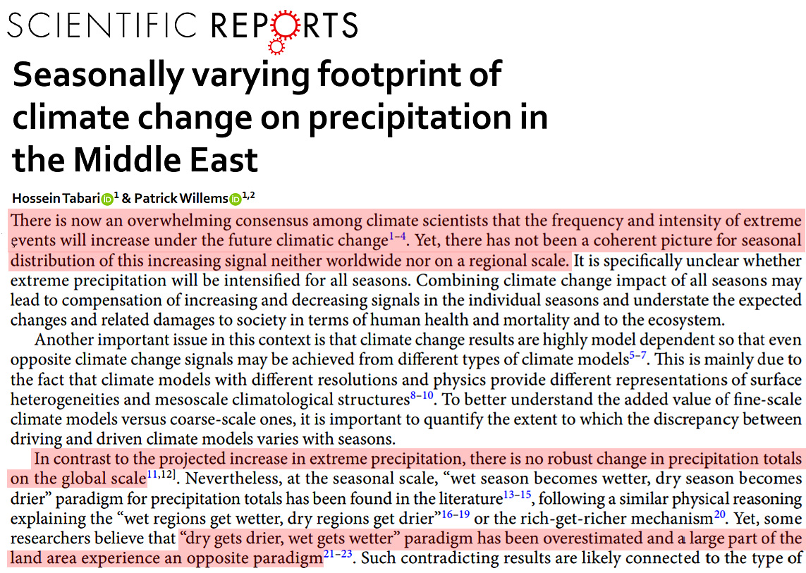
Peak Oil As Myth

Zapivalov, 2018     Hydrocarbons are reported to occur in all strata of the Earth’s crust and are supposed to occur in the cosmic space, too. … Oil-and-gas accumulations are traced in all types of rocks and at all stratigraphic levels both onshore and offshore. In fact, we live in a hydrocarbon civilization. Our planet is actually a large overall petroleum polygon.  New evidence and facts refuted the myth of “Peak Oil”. Oilfields can be discovered in most unexpected places and conditions. The oil recovery rates depend on various natural, technogenic, and market fluctuations including human factor. A great variety of hydrocarbon sources, both conventional and unconventional, have been discovered and are still being discovered; innovative methods and technologies for hydrocarbon production and utilization are being created; on the whole it shows that Peak Oil is dead. The era of hydrocarbon civilization will never end!

Ragheb, 2018     Two schools of thought exist about the origin of petroleum: a Western school suggesting that its origin is biogenic resulting from the decay of organic biological matter and stored in sedimentary basins near the Earth’s surface, and a Ukrainian-Russian school proposing that it is abiogenic with an inorganic origin deep within the Earth’s crust dating back to the time of the formation of the Earth.  The first suggestion implies a finite resource, whereas the second implies an almost unlimited one.  Each school dismisses the other one, leading to interesting discussions and discourses. … An argument for the existence of abiogenic petroleum is that the deepest fossil ever found has been about 16,000 feet below sea level, yet petroleum can be extracted from wells drilled down to 30,000 feet and more.  The argument is advanced that if a fossil was once living matter, it had to be on the surface.  If it did turn into petroleum, at or near the surface, and since petroleum has a lower density than water it would be expected to rise on top of water not go under it.  The counter-argument is that these deep deposits may have resulted from crustal movements or were buried by bolide impacts.

Konga, 2018     Consensus on the creation and origin of petroleum currently held by western science points to ancient microorganisms, plant matter and their subsequent burial over millions of years after which immense pressure and temperature caused by the material collecting on top of them resulted in transformation of solid, liquid and gas formations known as coal, oil and natural gas. This type of theory is referred to as biogenic or Western theory on the creation and origin of oil (Summers, 2015). However, there is a growing number of scientists and researchers challenging such a theory, indicating that organic compounds are extremely common in space rock and atmospheres of other planets in our solar system (Bansal, 2015), suggesting that these compounds must be abiogenic in origin rather than biogenic. … The opposing group of abiogenic theory supporters, also called Russian-Ukrainian group explain inorganic origin of oil because of chemical reactions of minerals rather than by decay of organic matter, further deducting that oil is a renewable resource found in immense quantities in presently unreachable depths (Ragheb, 2018). Hydrocarbons are a chemical compound consisting of a combination of hydrogen and carbon atoms, together in great quantities making up the composition of oil (EIA, 2017b). … Popularity of biogenic theory can be attributed to the 17th and 18th century scientific understanding of carbon-based compounds and importance of life in their creation (Summers, 2015). Additionally, different types of organic matter and residue was found in various depths and layers of rock formations deep underground, which combinedwith extreme pressure, temperature and other factors could have resulted in huge concentrated stores of oil, as extraction of oil from fossilised organic matter is proved true (Heinberg, 2018). … Although it is widely supported fact that oil can be retrieved from fossilised organisms (Penner, 2018) and is conjointly backed by decades of data and technological development, some newer research has proven that part of the chemistry suggested by the abiogenic theory supporters to be surprisingly valid and worth investigating.

Miscellaneous

Temperature Data Sets Are ‘Remarkably Different’, Produce ‘Conflicting Results’ With ‘Large Uncertainties’

Rao et al., 2018     Land Surface Air Temperature Data Are Considerably Different Among BEST‐LAND, CRU‐TEM4v, NASA‐GISS, and NOAA‐NCEI … Several groups routinely produce gridded land surface air temperature (LSAT) data sets using station measurements to assess the status and impact of climate change. The Intergovernmental Panel on Climate Change Fifth Assessment Report suggests that estimated global and hemispheric mean LSAT trends of different data sets are consistent. However, less attention has been paid to the intercomparison at local/regional scales, which is important for local/regional studies. In this study we comprehensively compare four data sets at different spatial and temporal scales, including Berkley Earth Surface Temperature land surface air temperature data set (BEST‐LAND), Climate Research Unit Temperature Data Set version 4 (CRU‐TEM4v), National Aeronautics and Space Administration Goddard Institute for Space Studies data (NASA‐GISS), and data provided by National Oceanic and Atmospheric Administration National Center for Environmental Information (NOAA‐NCEI). The mean LSAT [land surface air temperature] anomalies are remarkably different because of the data coverage differences, with the magnitude nearly 0.4°C for the global and Northern Hemisphere and 0.6°C for the Southern Hemisphere. This study additionally finds that on the regional scale, northern high latitudes, southern middle‐to‐high latitudes, and the equator show the largest differences nearly 0.8°C. These differences cause notable differences for the trend calculation at regional scales. At the local scale, four data sets show significant variations over South America, Africa, Maritime Continent, central Australia, and Antarctica, which leads to remarkable differences in the local trend analysis. For some areas, different data sets produce conflicting results of whether warming exists. Our analysis shows that the differences across scales are associated with the availability of stations and the use of infilling techniques. Our results suggest that conventional LSAT data sets using only station observations have large uncertainties across scales, especially over station‐sparse areas. … The relative difference of trends estimated from different data sets can reach nearly 90% for different regions and time periods. CRU-TEM4v generally appears to have the largest grid box scale differences, while NASA-GISS has the smallest differences compared to BEST-LAND. The uncertainty of the LSAT [land surface air temperature] trend estimation caused by the data set differences (i.e., RMSD) ranges from 0.035 to 0.086°C per decade for the long-term trend (i.e., 1901–2017) to 0.097–0.305°C per decade for recent decades (i.e., 1981–2017). … In developing future LSAT data sets, the data uncertainty caused by limited and unevenly distributed station observations must be reduced.

Large Regions Of The World Ocean Have Been Cooling…Just 0.02°C Change Since 1994

Wunsch, 2018    Lower-bounds on uncertainties in oceanic data and a model are calculated for the 20-year time means and their temporal evolution for oceanic temperature, salinity, and sea surface height, during the data-dense interval 1994–2013. … Trends are estimated as … 0.0011 ±  0.0001 °C/y [whole ocean temperature, 0.011°Cper decade], with formal 2-standard deviation uncertainties. The temperature change corresponds to a 20-year average ocean heating rate of  0.48 ±0.1 W/m2 of which 0.1 W/m2 arises from the geothermal forcing. … The mean slope implies a change over 20 years [1994-2013] of 0.0213 ± 0.0014 °C … Annual mean temperature anomalies integrated to different depths including the bottom in °C. Two standard deviation bars are derived from bootstrapping the full temperature difference field each year. Ttot is integrated top-to-bottom; T100m, T700m, T3600m are integrated to 100, 700, and 3600 m, respectively. Tabyss is integrated from 3600 m to the bottom. Cooling in the region below 3600 m was discussed by Wunsch and Heimbach (2014).

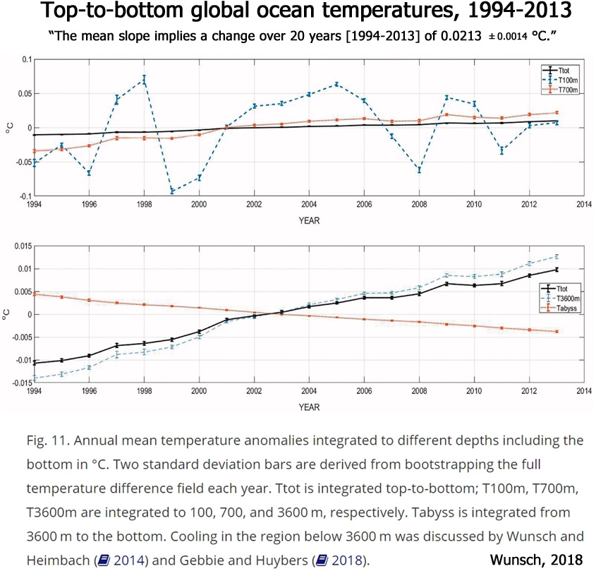
Climate Change Is Not A Problem…It’s Unframeable Philosophically

Campbell et al., 2018     Climate Change Is Not a Problem: Speculative Realism at the End of Organization … In this paper, we trace the compounding and escalation of frames to try and encompass the reality of climate change. These frames capture significant aspects, revealing new contours and extreme organizational challenges. However, what if climate change is unframeable? We locate three ontological dimensions of climate change – its unboundedness, incalculability and unthinkability – that make this case. This means that climate change is not a problem that organizations can encompass, divide or draw lines around – some ‘thing’ that can be recuperated into existing institutional, infrastructural and interpersonal frameworks. Instead, it is calling forth forms of organization without any precedent. We argue that the philosophy of speculative realism, specifically the work of Quentin Meillassoux, reveals climate change as a new World for which we do not have categories.

CO2 Growth Rate Follows Temperature Change

Chylek et al., 2018     We analyze monthly tropical near surface air temperature and Mauna Loa Observatory carbon dioxide (CO2) data within 1960–2016 to identify different carbon cycle responses for two El Nino types: El Ninos originating in the central tropical Pacific (CP El Nino) and El Ninos originating in the eastern tropical Pacific (EP El Nino). We find significant differences between the two types of El Nino events with respect to time delay of the CO2 rise rate that follows the increase in tropical near surface air temperatures caused by El Nino events. The average time lag of the CP El Nino is 4.0 ±1.7 months, while the mean time lag of EP El Nino is found to be 8.5±2.3 months. The average lag of all considered 1960–2016 El Ninos is 5.2±2.7 months. In contrast the sensitivity of the CO2 growth rate to tropical near surface air temperature increase is determined to be about the same for both El Nino types equal to 2.8±0.9 ppm yr−1K−1 (or 5.9±1.9 GtC yr−1K−1). Our results should be useful for the understanding of the carbon cycle and constraining it in climate models.

Exposure to 15,000 ppm CO2 Has No Detectable Effect On Human Cognition

Rodeheffer et al., 2018     Submarines routinely operate with higher levels of ambient carbon dioxide (CO2) (i.e., 2000 – 5000 ppm) than what is typically considered normal (i.e., 400 – 600 ppm). … The objective of this study was to determine if submariner decision-making performance is impacted by acute exposure to levels of CO2 routinely present in the submarine atmosphere during sea patrols. (1) METHODS: Using a subject-blinded balanced design, 36 submarine-qualified sailors were randomly assigned to receive 1 of 3 CO2 exposure conditions (600, 2500, or 15,000 ppm). After a 45-min atmospheric acclimation period, participants completed an 80-min computer-administered SMS test as a measure of decision making. (2) RESULTS: There were no significant differences for any of the nine SMS measures of decision making between the CO2 exposure conditions. (3) DISCUSSION: In contrast to recent research demonstrating cognitive deficits on the SMS test in students and professional-grade office workers, we were unable to replicate this effect in a submariner population-even with acute CO2 exposures more than an order of magnitude greater than those used in previous studies that demonstrated such effects.

63% (Not 97%) Of German Climate Scientists Agree With IPCC ‘Consensus’

Post and Ramirez, 2018     The [131] German climate scientists largely confirm anthropogenic climate change. Almost two-thirds (63%) believe that “the climatic development in the past 50 years was predominantly influenced by human behavior,” and about a third (30%) believe it was “equally influenced by human behavior and natural factors.”Only one (1%) of the 131 climate scientists believe that it was “predominantly influenced by natural factors.” The rest (6%) did not answer the question or thinks that “this is hard to say.”

Ozone ‘Hole’ Still Widening Since 1998 (Despite CFC Ban) 

Ball et al, 2018     Here we report evidence from multiple satellite measurements that ozone in the lower stratosphere between 60° S and 60° N has indeed continued to decline since 1998. We find that, even though upper stratospheric ozone is recovering, the continuing downward trend in the lower stratosphere prevails, resulting in a downward trend in stratospheric column ozone between 60° S and 60° N. We find that total column ozone between 60° S and 60° N appears not to have decreased only because of increases in tropospheric column ozone that compensate for the stratospheric decreases. The reasons for the continued reduction of lower stratospheric ozone are not clear; models do not reproduce these trends, and thus the causes now urgently need to be established.

Arctic Methane Emissions Natural, Not Anthropogenic

Wallmann et al., 2018     Gas hydrate dissociation off Svalbard induced by isostatic rebound rather than global warming … Methane seepage from the upper continental slopes of Western Svalbard has previously been attributed to gas hydrate dissociation induced by anthropogenic warming of ambient bottom waters. Here we show that sediment cores drilled off Prins Karls Foreland contain freshwater from dissociating hydrates. However, our modeling indicates that the observed pore water freshening began around 8 ka BP when the rate of isostatic uplift outpaced eustatic sea-level rise. The resultant local shallowing and lowering of hydrostatic pressure forced gas hydrate dissociation and dissolved chloride depletions consistent with our geochemical analysis. Hence, we propose that hydrate dissociation was triggered by postglacial isostatic rebound rather than anthropogenic warming.

Switching To Natural Gas ‘Clearest Means’ To Reduce CO2 Emissions

Anderson et al., 2018     Before considering the future, it is worth examining just how far we’ve already come without any federal CO2 regulation (for existing power plants) in the U.S. Figure 1 illustrates historical CO2 emissions and natural gas prices from 2005 through 2017 (estimated). During that period, emissions have declined from nearly 2.7 billion tons to approximately 1.9 billion tons (∼30%), while revealing a strong link to natural gas prices. To be sure, while other factors (such as renewable energy incentives) also had an impact, the clearest means by which to reduce CO2 emissions has been to reduce the cost of generating electricity with less CO2-emitting fuels (i.e., substituting natural gas for coal). So successful have market forces been under the existing regulatory framework to date that estimated 2017 CO2 emission levels are already at the CPP’s 2025 target (albeit without accounting for electricity demand growth between 2017 and 2025), well exceeding the AEO’s own Reference Case projections for 2025.

The ‘Fakegate’ Scandal & AGW Advocates’ Unethical Hyping Of Climate Threats 

Olson, 2018      [O]pinion polls and other research show a public that frequently perceives climate science and associated AGW threats as complicated, uncertain and temporally and spatially distant (Anghelcev et al., 2015; Bennett et al., 2016; Gordon et al., 2011). Thus climate scientists, celebrities, public policymakers and other AGW social marketers face a daunting task in convincing a lackadaisical and often skeptical public to support AGW mitigating behaviors and policies. The difficulty of this marketing assignment has also led to the utilization of ethically questionable tactics that hype the severity, immediacy and certainty of AGW threats (O’Neil and Nicholson-Cole, 2009; Rogers, 1975; Rosenberg et al., 2010).

For example, the past 25 years have witnessed a large number of greatly exaggerated predictions regarding the speed and scope of temperature increases and AGW dangers from a variety of AGW “endorsers,” which have fortunately proven to be false alarms (Bastasch, 2015; Grundmann, 2011; Michaels, 2008; Newman, 2014).  Another ethically questionable example is provided by the Climategate scandal involving members of the climate science community and their attempts to increase public certainty regarding the methods and predictions of “mainstream” climate models by blocking the publication of research not supportive of the AGW paradigm (Curry, 2014; Grundmann, 2011).

The Fakegate scandal that is the focus of the current research is different than other AGW scandals and ethical missteps, however, because the protagonist publicly admitted to the intentional use of ethically questionable tactics for the purposes of favorably influencing public opinion regarding the AGW cause. Fakegate started with the theft of internal strategy and donor documents from the Heartland Institute, a libertarian think tank and dangerous AGW “competitor” owing to their efforts to educate the public regarding climate model uncertainties and the high economic and political costs of AGW mitigation (Hoffman, 2011). … An analysis of the writing style, content details and errors in the fake document led several bloggers to speculate that the thief and fake document author was Peter Gleick, a climate researcher, environmental think tank president, chairman of a scientific association ethics committee and frequent blogger on climate science and AGW threats (Greenhut, 2012). These publicly discussed suspicions led Gleick to confess and apologize for his use of deception in posing as a Heartland board member to acquire and disseminate the internal documents.

Failures provide valuable learning opportunities, and the Fakegate failure demonstrates that social marketers who are unwilling or unable to honestly and persuasively debate the scientific validity and “greater good” of their cause, should not resort to ethically questionable persuasion tactics if they hope to win widespread and lasting trust and support for their social marketing objectives. The current study also makes a contribution through its close examination of AGW skeptic arguments that have typically been ignored or dismissed (Hoffman, 2011; Koteyko et al., 2013). In contrast to the scientific ignorance commonly attributed to skeptics, the sophistication and apparent validity of their viewpoints regarding scientific progress and the high costs of AGW mitigation suggest that skeptics more than deserve the respect, transparency and inclusion that social marketing ethical guidelines promote, but which many AGW social marketers have failed to follow.

‘Stable Or Increasing’ Species Richness, -0.02°C Century-Scale Cooling (California)

MacLean et al., 2018     A century of climate and land‐use change cause species turnover without loss of beta diversity in California’s Central Valley Climate and land‐use changes are thought to be the greatest threats to biodiversity, but few studies have directly measured their simultaneous impacts on species distributions. We used a unique historic resource—early 20th‐century bird surveys conducted by Joseph Grinnell and colleagues—paired with contemporary resurveys a century later to examine changes in bird distributions in California’s Central Valley, one of the most intensively modified agricultural zones in the world and a region of heterogeneous climate change. … At the community level, we found no significant change in average occupancy or in species richness per site. This result contradicts expectations that occupancy and richness should decrease at sites experiencing anthropogenic land‐use and climate change (Distler et al., 2015; McKinney, 2002; Newbold et al., 2015; Wiens, Stralberg, Jongsomjit, Howell, & Snyder, 2009). … This counterintuitive pattern of stable or increased site‐level species richness has been documented elsewhere (Dornelas et al., 2014; Sax & Gaines, 2003) but is unusual for a study region like ours that has undergone dramatic increases in urbanization and agriculture during the century between our surveys (Cardinale, 2011; Frishkoff et al., 2016; Karp et al., 2017; Karp, Ziv, Zook, Ehrlich, & Daily, 2011).  … Historic surveys occurred between 1912 and 1923 (late March through June). … We conducted modern resurveys during the breeding seasons (April through June) of 2015 and 2016.  The average (±1 SE) maximum temperature across all sites did not change significantly (historic [1912-’23]: 31.9 ± 1.5°C; modern [2015-’16]: 31.7 ± 1.5°C), but change varied greatly among sites from +1.1°C to −2.3°C. Both patterns were similar to trends in maximum temperature that occurred throughout California during the 20th century (Rapacciuolo et al., 2014). Mean annual precipitation increased slightly from 3.4 ± 2.9 to 4.1 ± 3.3 cm, which was less than the increase of 2.7 cm average across the entire state.

Has The ‘Little Ice Age’ Returned in Japan?

Collins, 2018     Evidence that the long-predicted “Little Ice Age” has started is now accumulating rapidly. This is the opposite phenomenon from “Anthropogenic Global Warming” (AGW) to prepare for which Japan spends several Trillion Yen/year. Although there are many uncertainties about the Earth’s climate, it is clear that, contrary to AGW predictions, the Earth’s atmosphere has not warmed at all for 20 years. Moreover, the increase in recent years in Japan of “Guerilla Rainstorms” followed by “Guerilla Snowstorms” and now the coldest winter in 50 years are as predicted by Russian astrophysicists, in contrast to AGW advocates’ predictions. … Recent major advances in the technology used to produce coal, oil and natural gas, combined with growing acceptance of the theory of “Non-Abiotic” Oil and Gas, contradict the long-standing idea that “supplies of oil and gas will soon run out” which mass-media have been spreading for the past 30 years. Consequently humans’ ever-growing energy demand no longer seems a major problem, and so it is no longer possible to argue that SPS is urgently needed to supply electricity after the exhaustion of “fossil fuels”, which has been the main argument for developing “Solar Power Satellites” (SPS) since they were first proposed in 1968.

A Decline In CO2 Below 450 ppm May Have Triggered Species Extinctions

Faith et al., 2018     Human ancestors have been proposed as drivers of extinctions of Africa’s diverse large mammal communities. Faith et al. challenge this view with an analysis of eastern African herbivore communities spanning the past ∼7 million years (see the Perspective by Bobe and Carvalho). Megaherbivores (for example, elephants, rhinos, and hippos) began to decline about 4.6 million years ago, preceding evidence for hominin consumption of animal tissues by more than 1 million years. Instead, megaherbivore decline may have been triggered by declining atmospheric carbon dioxide and expansion of grasslands. … Because C4 grasses are favored at lower CO2 concentrations [Ehleringer et al., 1997], the Plio-Pleistocene CO2 decline (Fig. 2A) is likely an important abiotic mechanism [Levin, 2015]. For example, at high temperatures, such as those inferred from Turkana Basin paleosol carbonates (>30°C) (28), C4 grasses are expected to expand when atmospheric CO2 concentrations fall below ~450 parts per million [Ehleringer et al., 1997]. The expansion of C4 grasslands and associated decline of megaherbivores are consistent with long-term decline of CO2 (Fig. 2), likely facilitated by episodes of aridity (i.e., positive water deficit) that occurred across the interval (Fig. 2C).

(press release)   “Our analyses show that there is a steady, long-term decline of megaherbivore diversity beginning around 4.6 million years ago. This extinction process kicks in over a million years before the very earliest evidence for human ancestors making tools or butchering animal carcasses and well before the appearance of any hominin species realistically capable of hunting them, like Homo erectus,” says Faith.

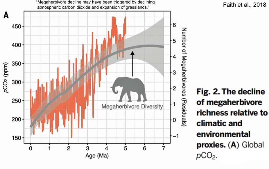
‘Perhaps Half’ Of Peer-Reviewed Science ‘Has Significant Flaws’

Lacrombe and Ridd, 2018     Research science used to inform public policy decisions, herein defined as “Policy-Science”, is rarely subjected to rigorous checking, testing and replication. Studies of biomedical and other sciences indicate that a considerable fraction of published peer-reviewed scientific literature, perhaps half, has significant flaws. To demonstrate the potential failings of the present approaches to scientific Quality Control (QC), we describe examples of science associated with perceived threats to the Great Barrier Reef (GBR), Australia.

Equilibrium Climate Sensitivity 1.66 K, Models Are ‘Inconsistent With Observed Warming’

Lewis and Curry, 2018     Using an 1869–82 base period and a 2007–16 final period, which are well matched for volcanic activity and influence from internal variability, medians are derived for ECS of 1.50 K (5%–95% range: 1.05–2.45 K) and for TCR of 1.20 K (5%–95% range: 0.9–1.7 K). These estimates both have much lower upper bounds than those from a predecessor study using AR5 data ending in 2011. Using infilled, globally complete temperature data give slightly higher estimates: a median of 1.66 K for ECS (5%–95% range: 1.15–2.7 K) and 1.33 K for TCR (5%–95% range: 1.0–1.9 K). These ECS estimates reflect climate feedbacks over the historical period, assumed to be time invariant. Allowing for possible time-varying climate feedbacks increases the median ECS estimate to 1.76 K (5%–95% range: 1.2–3.1 K), using infilled temperature data. Possible biases from non–unit forcing efficacy, temperature estimation issues, and variability in sea surface temperature change patterns are examined and found to be minor when using globally complete temperature data. These results imply that high ECS and TCR values derived from a majority of CMIP5 climate models are inconsistent with observed warming during the historical period.

Scientists Confused About Venus: Heat Loss Mechanism Estimates Off By Factor Of Two

O’Rourke and Smrekar, 2018     We searched for but failed to find systematic differences in plate thickness as functions of the geologic setting or extent of tectonic fractures. In general, we calculated heat flows that are larger than the global average on present‐day Earth—roughly twice typical values predicted for Venus, which may cool slowly or even heat up absent plate tectonics. Therefore, we conclude that coronae are sites of above average heat flow on Venus and in fact contribute a significant portion of the total heat loss budget.

(press release)      How does Venus, a planet similar in size to the Earth, lose heat? This question is at the heart of a long-standing conundrum of how these two planets of similar make up became so starkly different.  … Their analysis indicates that the heat loss from most coronae exceeds the average expected on Venus, often by a factor of two or more. While coronae only cover approximately four percent of the surface of the planet, O’Rourke and Smrekar find that they may account for 25 percent or more of the total heat loss. Thus, coronae are a crucial component of how Venus loses heat and how its surface and interior evolves.