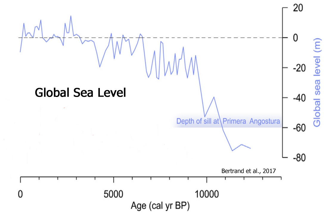
Lack Of Anthropogenic/CO2 Signal In Sea Level Rise (39)
No Net Warming During 20th (21st) Century (13)
A Warmer Past: Non-Hockey Stick Reconstructions (60)
Abrupt, Degrees-Per-Decade Natural Global Warming (7)
A Model-Defying Cryosphere, Polar Ice (34)
Antarctic Ice Melting In High Geothermal Heat Flux Areas (4)
Recent Cooling In The North Atlantic, Southern Ocean (10)
Part 3. Natural Climate Change Observation, Reconstruction
Lack Of Anthropogenic/CO2 Signal In Sea Level Rise (38)
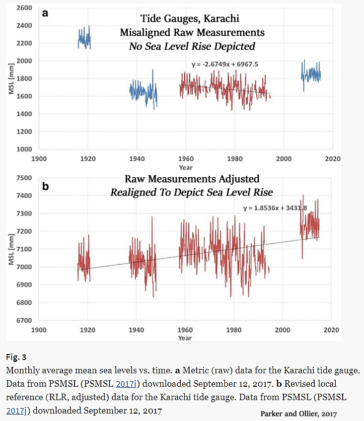
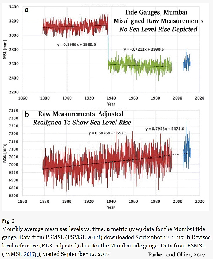
Parker and Ollier, 2017 [L]ocal sea-level forecasts should be based on proven local sea-level data. Their naïve averaging of all the tide gauges included in the PSMSL surveys showed ‘‘relative’’ trends of about + 1.04 mm/year (570 tide gauges of any length). By only considering the 100 tide gauges with more than 80 years of recording, the average trend was only + 0.25 mm/year [2.5 centimeters per century]. … The loud divergence between sea-level reality and climate change theory—the climate models predict an accelerated sea-level rise driven by the anthropogenic CO2 emission—has been also evidenced in other works such as Boretti (2012a, b), Boretti and Watson (2012), Douglas (1992), Douglas and Peltier (2002), Fasullo et al. (2016), Jevrejeva et al. (2006), Holgate (2007), Houston and Dean (2011), Mörner 2010a, b, 2016), Mörner and Parker (2013), Scafetta (2014), Wenzel and Schröter (2010) and Wunsch et al. (2007) reporting on the recent lack of any detectable acceleration in the rate of sea-level rise. The minimum length requirement of 50–60 years to produce a realistic sea-level rate of rise is also discussed in other works such as Baart et al. (2012), Douglas (1995, 1997), Gervais (2016), Jevrejeva et al. (2008), Knudsen et al. (2011), Scafetta (2013a, b), Wenzel and Schröter (2014) and Woodworth (2011). … [T]he information from the tide gauges of the USA and the rest of the world when considered globally and over time windows of not less than 80 years […] does not support the notion of rapidly changing mass of ice in Greenland and Antarctica as claimed by Davis and Vinogradova (2017). The sea levels have been oscillating about a nearly perfectly linear trend since the start of the twentieth century with no sign of acceleration. There are only different phases of some oscillations moving from one location to another that do not represent any global acceleration. …The global sea-level acceleration is therefore in the order of + 0.002 ± 0.003 mm/year², i.e. + 2 ÷ 3 μm/year², well below the accuracy of the estimation. This means that the sea levels may rise in the twenty-first century only a few centimeters more than what they rose during the twentieth century. This is by no means alarming.
Parker and Ollier, 2017 The tide gauge result of Aden is perfectly consistent not only with the tide gauge results for Karachi and Mumbai. It is also consistent with the multiple lines of evidence, tide gauges, coastal morphology, stratigraphy, radiocarbon dating, archaeological remains, and historical documentation, for a stable sea level of about zero mm/year experienced over the last 50 years in all the key sites of the Indian Ocean (Mörner 2007, 2010, 2014, 2015a, b, 2016a, b). … Contrary to the adjusted data from tide gauges and the unreliable satellite altimeter data, properly examined data from tide gauges and other sources such as coastal morphology, stratigraphy, radiocarbon dating, archaeological remains, and historical documentation indicate a lack of any alarming sea-level rise in recent decades for all the Indian Ocean. In both cases, it was shown that the latest positive trends in the PSMSL RLR [revised local reference, adjusted] data are only the result of arbitrary alignments, and alternative and more legitimate alignments reveal very stable sea-level conditions. The metric (raw) data show misaligned results. The metric data are the data as originally provided, or suffering from historical adjustments. What are more dangerous are the corrections recently introduced to the past to magnify the sea-level trend or the acceleration. … While the metric data do not tell us, which is the correct trend, they tell us that the alignments made to produce the RLR [revised local reference, or adjusted data] are very likely wrong, because they are inconsistent with the individual measurements components, none of which showing any sign of increasing sea levels, and because the adjustments are always in the direction to produce a large rise in sea level.
Mörner, 2017 Coastal morphology, stratigraphy, radiocarbon dating, archaeological remains, historical documentation, and tide gauge records allowed us to establish a very firm and detailed record of the changes in sea level in Goa over the last 500 years. It is an oscillation record: a low level in the early 16th century, a ~50-cm high[er than now] level in the 17th century, a level below present sea level in the 18th century, a ~20-cm high level in the 19th and early 20th centuries, a ~20-cm fall in 1955–1962, and a virtually stable level over the last 50 years. This sea level record is almost identical to those obtained in the Maldives and in Bangladesh. The Indian Ocean seems to lack records of any alarming sea-level rise in recent decades; on the contrary, 10 sites analyzed indicate a sea level remaining at about 60.0, at least over the last 50 years or so.
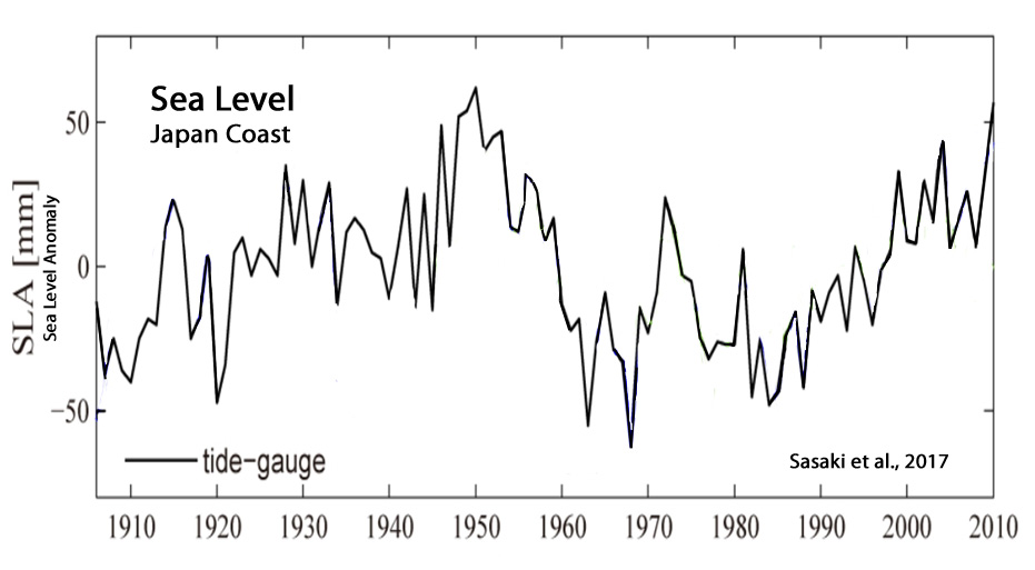
Sasaki et al., 2017 Sea level variability around Japan from 1906 to 2010 is examined using a regional ocean model, along with observational data and the CMIP5 historical simulations. The regional model reproduces observed interdecadal sea level variability, e.g., high sea level around 1950, low sea level in the 1970s, and sea level rise during the most recent three decades, along the Japanese coast. Sensitivity runs reveal that the high sea level around 1950 was induced by the wind stress curl changes over the North Pacific, characterized by a weakening of the Aleutian Low. In contrast, the recent sea level rise is primarily caused by heat and freshwater flux forcings. That the wind-induced sea level rise along the Japanese coast around 1950 is as large as the recent sea level rise highlights the importance of natural variability in understanding regional sea level change on interdecadal timescales.
Montecino et al., 2017 Our estimation of the SLC in the Chilean coast revealed an overall increase in sea level. The sea level in Chile does not strictly follow the global trend of the past two decades (~3 mm year−1), but rather a slight agreement (from 1.2 to 0.6 mm year−1) from Arica up to Puerto Montt approximately, with the exception of PTAR and PWIL TGs, where we found a decrease of −0.9 and −0.8 mm year−1, respectively.
Rani et al., 2017 In the present study, an attempt has been made to understand the variability of mean sea level (MSL) over east and west coast of India during 1973–2010. … The observations also reveal an increase of 1.353 mm/year on the east coast and observed a total 0.372 mm/ year on the west coast.
Parekh et al., 2017 The rate of sea level rise over the Arabian Sea is about 0.5–3 mm/year, whereas over the Bay of Bengal, it is 0.75–6 mm/year. Major contributors to these changes in the Indian Ocean are steric effect and short-term climate variability such as El Niño–Southern Oscillation (ENSO) and the Indian Ocean Dipole. This affirms that sea level trends over north Indian Ocean get modulated by inter-annual and decadal scale natural climate variability. The inter-annual variability is stronger than decadal variability, which in turn is stronger than the long-term sea level trend. Sea level change in the Indian Ocean is about 1.5 mm/year in the past sixty years or so, whereas the global sea level trends are a bit higher.
McAneney et al., 2017 Global averaged sea-level rise is estimated at about 1.7 ± 0.2 mm year−1 (Rhein et al. 2013), however, this global average rise ignores any local land movements. Church et al. (2006) and J. A. Church (2016; personal communication) suggest a long-term average rate of relative (ocean relative to land) sea-level rise of ∼1.3 mm year. …The data show no consistent trend in the frequency of flooding over the 122-year [1892-2013] duration of observations despite persistent warming of air temperatures characterized in other studies. On the other hand, flood frequencies are strongly influenced by ENSO phases with many more floods of any height occurring in La Niña years. … In terms of flood heights, a marginal statistically significant upward trend is observed over the entire sequence of measurements. However, once the data have been adjusted for average sea-level rise of 1.3 mm year−1 over the entire length of the record, no statistically significance remains, either for the entire record, or for the shortened series based on higher quality data. The analysis of the uncorrected data shows how the choice of starting points in a time series can lead to quite different conclusions about trends in the data, even if the statistical analysis is consistent. … In short, we have been unable to detect any influence of global warming at this tropical location on either the frequency, or the height of major flooding other than that due to its influence on sea-level rise.
Zerbini et al., 2017 Our study focuses on the time series of Alicante, in Spain, Marseille, in France, Genoa, Marina di Ravenna (formerly Porto Corsini), Venice and Trieste, in Italy. After removing the vertical land motions in Venice and Marina di Ravenna, and the inverted barometer effect at all the sites, the linear long period sea-level rates were estimated. The results are in excellent agreement ranging between + 1.2 and + 1.3 mm/year for the overall period from the last decades of the 19th century till 2012. The associated errors, computed by accounting for serial autocorrelation, are of the order of 0.2–0.3 mm/year for all stations, except Alicante, for which the error turns out to be 0,5 mm/year. … Our estimated rates for the northern Mediterranean, a relatively small regional sea, are slightly lower than the global mean rate, + 1.7 ± 0.2 mm/year, recently published in the IPCC AR5 (Intergovernmental Panel on Climate Change 5th Assessment Report) (Church et al., 2013), but close enough, if uncertainties are taken into account. It is known that Mediterranean stations had always had lower trends than the global-average ones. Our regional results, however, are in close agreement with the global mean rate, + 1.2 mm/year, published by Hay et al. (2015) which is currently being discussed by the oceanographic community
Watson, 2017 The analysis in this paper is based on a recently developed analytical package titled ‘‘msltrend,’’ specifically designed to enhance estimates of trend, real-time velocity, and acceleration in the relative mean sea-level signal derived from long annual average ocean water level time series. Key findings are that at the 95% confidence level, no consistent or compelling evidence (yet) exists that recent rates of rise are higher or abnormal in the context of the historical records available across Europe, nor is there any evidence that geocentric rates of rise are above the global average. It is likely a further 20 years of data will distinguish whether recent increases are evidence of the onset of climate change–induced acceleration.
Mörner, 2017 [T]he stratigraphic and morphological records documented in the coastal area of the islands of Garaidhoo and Lhosfushi in the South Male Atoll, provide sea level information partly of a rapid sea level rise from about ±0 in the 12th century to about +60 cm [above present] in the 13th century [+6 mm/yr], and partly of three subsequent levels of +50 – 60 cm in the 17th century, +20 cm in the 19th and 20th centuries and then a fall to present sea level in the 1970s, which is in full agreement with records from other sites in the Indian Ocean (and even in the Fiji Islands according to new data).
Bezdek, 2017 Land subsidence in the Chesapeake Bay region was first documented over four decades ago by Holdahl and Morrison who reported results of geodetic surveys completed between 1940 and 1971 and found land surfaces across the region were sinking at an average rate of 2.8 mm/yr. with rates ranging from 1.1 to 4.8 mm/yr. … … [G]lobal average sea levels have been rising at about 1.8 mm/yr. Although rates of absolute sea-level rise (rise due just to increases in ocean volume) can vary substantially from one location to another and change over time, the global average rate of 1.8 mm/yr. from 1961 to 2003 is a widely accepted global benchmark rate. … [T]he difference between average subsidence rate of about 3.1 mm/yr and the average estimated sea-level rise computed in the Chesapeake Bay area of about 3.9 mm/yr. is 0.8 mm/year. These data indicate that land subsidence has been responsible for most of the relative sea-level rise measured in the Chesapeake Bay region over the past half-century. … Sea level rise due to climate change is a contentious issue with profound geographic and economic implications, and there is little doubt that water intrusion is a serious problem in much of the Chesapeake Bay region. However, the critical question is whether this water intrusion is the result of climate-induced sea level rise or is being caused by other factors. Our findings indicate that the water intrusion problems in the region are due not to “sea level rise”, but, rather, primarily to land subsidence due to groundwater depletion and, to a lesser extent, subsidence from glacial isostatic adjustment. We conclude that water intrusion may thus continue even if sea levels actually decline.
Eghbert et al., 2017 In September 2015, altimetry data show that sea level was at its lowest in the past 12 years [Indonesia], affecting corals living in the bathymetric range exposed to unusual emersion. In March 2016, Bunaken Island (North Sulawesi) displayed up to 85% mortality on reef flats dominated by Porites, Heliopora and Goniastrea corals with differential mortality rates by coral genus. … [R]apid sea level fall could be more important in the dynamics and resilience of Indonesian reef flat communities than previously thought. This study reports coral mortality in Indonesia after an El Niño-induced sea level fall. The fact that sea level fall, or extremely low tides, induces coral mortality is not new, but this study demonstrates that through rapid sea level fall, the 2015–2016 El Niño has impacted Indonesian shallow coral reefs well before high sea surface temperature could trigger any coral bleaching. Sea level fall appears as a major mortality factor for Bunaken Island in North Sulawesi, and altimetry suggests similar impact throughout Indonesia.
Munshi, 2017 Detrended correlation analysis of a global sea level reconstruction 1807-2010 does not show that changes in the rate of sea level rise are related to the rate of fossil fuel emissions at any of the nine time scales tried. The result is checked against the measured data from sixteen locations in the Pacific and Atlantic regions of the Northern Hemisphere. No evidence could be found that observed changes in the rate of sea level rise are unnatural phenomena that can be attributed to fossil fuel emissions. These results are inconsistent with the proposition that the rate of sea level rise can be moderated by reducing emissions. It is noted that correlation is a necessary but not sufficient condition for a causal relationship between emissions and acceleration of sea level rise.
Parker and Ollier, 2017 We show that the sea level rises estimate by a local panel for California as well as the IPCC for the entire world are up to one order of magnitude larger than what is extrapolated from present sea level rise rates and accelerations based on tide gauge data sets. These extrapolations are consistent with present temperature warming rates and accelerations of different global temperature data sets (University of Alabama in Huntsville UAH and Remote Sensing Systems RSS) and IPCC Assessment Report (AR) 5 Representative Concentration Pathway (RCP) 8.5 sensitivity. As the evidence from the measurements does not support the IPCC expectations or the even more alarming predictions by the local California panel, these claims and the subsequent analyses are too speculative and not suitable for rigorous use in planning or policy making.
Mörner, 2017 Global tide gauge data sets may vary between +1.7 mm/yr to +0.25 mm/yr depending upon the choice of stations. At numerous individual sites, available tide gauges show variability around a stable zero level. Coastal morphology is a sharp tool in defining ongoing changes in sea level. A general stability has been defined in sites like the Maldives, Goa, Bangladesh and Fiji. In contrast to all those observations, satellite altimetry claim there is a global mean rise in sea level of about 3.0 mm/yr. In this paper, it is claimed that the satellite altimetry values have been “manipulated”. In this situation, it is recommended that we return to the observational facts, which provides global sea level records varying between ±0.0 and +1.0 mm/yr; i.e. values that pose no problems in coastal protection.
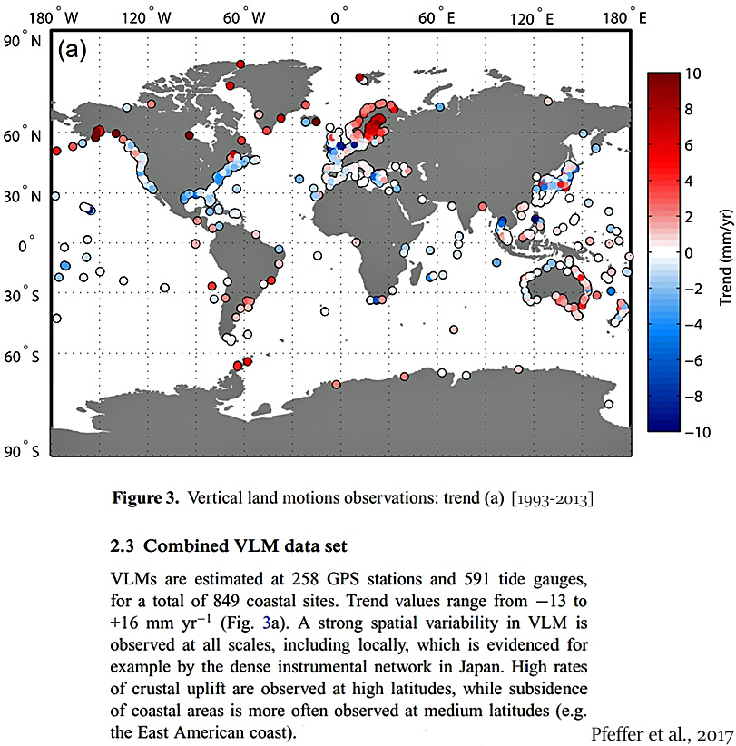
Pfeffer et al., 2017 VLMs contribute actively to the sea-level changes felt by coastal populations, as they can amplify, diminish or counteract the effects of climate-induced signals (e.g. Pfeffer & Allemand 2016). In many cases, for example, Torres Islands (Ballu et al. 2011), western Tropical Pacific (Becker et al. 2012), southern Europe(Woppelmann & Marcos ¨ 2012) or Indian Ocean (Palanisamy et al. 2014), VLMs[vertical land motions] have been recognized as a dominant component of the total relative sea-level variations observed at coasts. … VLMs are estimated at 258 GPS stations and 591 tide gauges, for a total of 849 coastal sites. Trend values range from −13 to +16 mm yr−1 (Fig. 3a). A strong spatial variability in VLM is observed at all scales, including locally, which is evidenced for example by the dense instrumental network in Japan. High rates of crustal uplift are observed at high latitudes, while subsidence of coastal areas is more often observed at medium latitudes (e.g. the East American coast).
Holocene Sea Levels Much Higher When CO2 Levels Much Lower
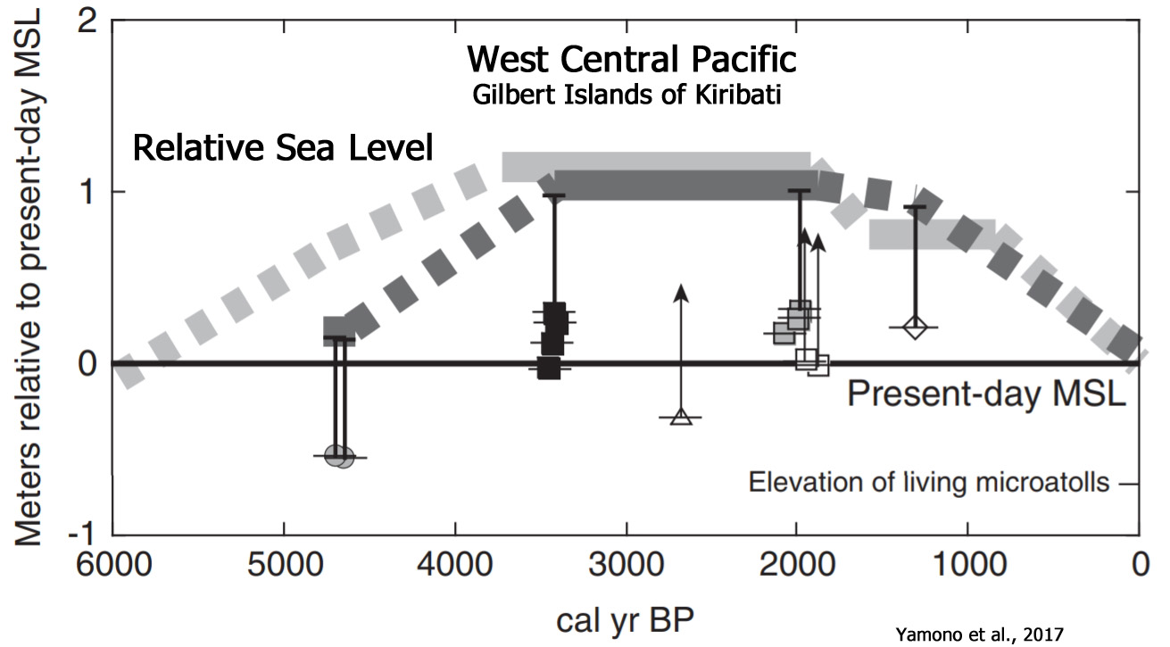
Yamono et al., 2017 New coral microatoll data allow presenting an updated late Holocene sea-level curve for the Gilbert Islands of Kiribati. Examination of build-up elevation and spatial distribution of microatolls, along with radiocarbon age data from coral samples, suggest an approximately 1 m sea-level high stand [above present], possibly lasting from ~3500 to 1900 cal yr BP. … By radiocarbon dating fossil corals and Tridacna shells at several locations, Schofield (1977) showed that in the late Holocene, sea level in this region was approximately 2.4 m higher than at present, and also suggested that sea-level oscillations have occurred, with six transgressions during the last 5000 yr.
Cooper et al., 2017 Whitepark Bay is located on the paraglacial north coast of Northern Ireland. … After deglaciation sea-level fell to a low of -30 m by ca. 13.5 ka cal yr BP (Cooper et al., 2002; Kelley et al., 2006) before rising to a mid-Holocene highstand of 2-3 m above present around 6 cal kay r BP (Carter, 1982; Orford et al., 2006).
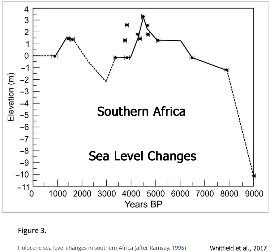
Whitfield et al., 2017 The estuarine lagoon would have been deeper than the present-day Groenvlei [Southern Africa], especially during the mid-Holocene sea level highstand about 4,500 BP when the sea level was 3.5 m higher than present (Ramsay, 1995), and the lagoon would have been fully tidal in synchrony with the main Swartvlei Estuary to the west. … A subsequent rise in sea level to +1.5 m [above present] about 1,600 years BP (Ramsay, 1995) would have been insufficient to breach the stabilized dune field that was isolating Groenvlei from the Swartvlei Estuary.
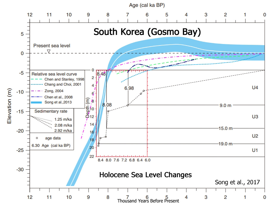
Song et al., 2017
Lecea et al., 2017 Ramsay (1995) produced a 9 kyr BP record of sea-level changes from the South African east coast, that showed sea levels reached a high stand of +3.5 m [above present] at 4.65 kyr BP. Similar high stands have been recorded elsewhere in the Southern Hemisphere, on the west coast of South Africa (0 – 3 m [above present], Compton, 2001), in south Australia (1 – 3 m [above present], Belperio et al., 2002), south- and north-east Australia (1.7 m [above present], Baker et al., 2001; 2 m [above present], Larcombe et al., 1995, respectively) and Brazil (2.1 m [above present], Angulo et al., 2006). In South Africa this was followed by a drop below present level before rising to another high stand at 1.6 kyr BP (Compton, 2001; Ramsey, 1995). … In Mozambique, Norström et al., (2012) identified a sea-level highstand ~3 m above present at ~ 6.6 kyr BP.

Das et al., 2017 In the absence of any evidence of land-level changes, the study suggests that at around 6 ka to 3 ka [6,000 to 3,000 years ago], the sea was approximately 2 m higher than present.
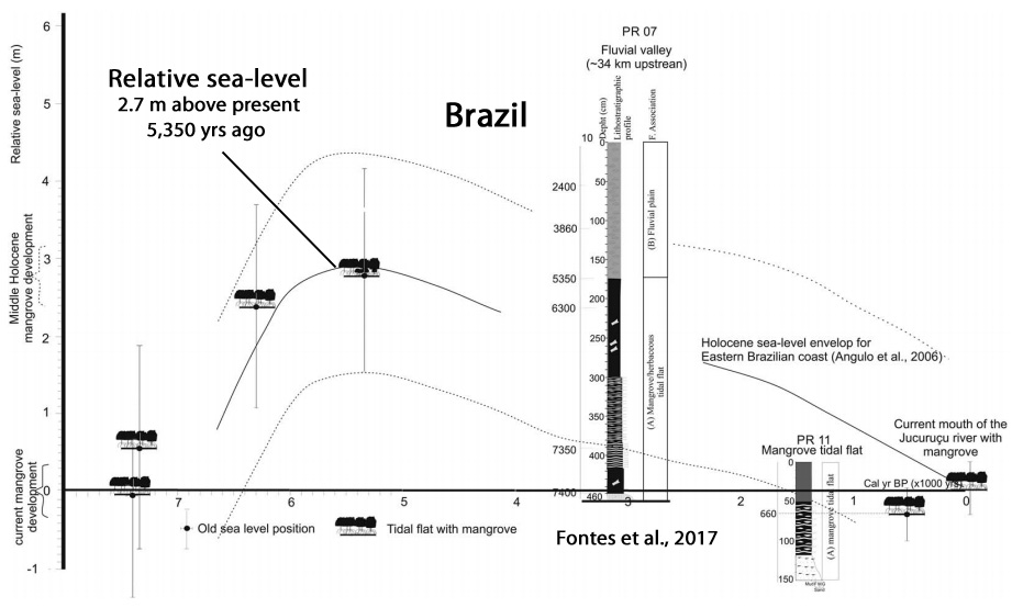
Fontes et al., 2017 During the early-middle Holocene there was a rise in RSL [relative sea level] with a highstand at about 5350 cal yr BP [calendar years before present] of 2.7 ± 1.35 m [higher than present], which caused a marine incursion along the fluvial valley.
Yoon et al., 2017 Songaksan is the youngest eruptive centre on Jeju Island, Korea, and was produced by a phreatomagmatic eruption in a coastal setting c. 3.7 ka BP [3,700 years before present]. The 1 m thick basal portion of the tuff ring shows an unusually well-preserved transition of facies from intertidal to supratidal, from which palaeo-high-tide level and a total of 13 high-tide events were inferred. Another set of erosion surfaces and reworked deposits in the middle of the tuff ring, as high as 6 m above present mean sea level, is interpreted to be the product of wave reworking during a storm-surge event that lasted approximately three tidal cycles. … The reworked deposits alternate three or four times with the primary tuff beds of Units B and C and occur as high as 6 m above present mean sea level or 4 m above high-tide level (based on land-based Lidar terrain mapping of the outcrop surface).
Bini et al., 2017 The main conclusion is that the relative sea-level between c. 7000 and 5300 cal. yr BP was in the range of c. 2–4 m a.s.l. [above present mean sea level], with a mean value of c. 3.5 m a.s.l. … Initial glacio-hydro-isostatic models of the Patagonian coast [Argentina] suggested that the shoreline could be characterized by currently raised beaches, which started to form as soon as ice-sheet melting ceased (Clark et al., 1978). A more recent model (Milne and Mitrovica, 2008) predicted that RSLs [relative sea levels] might have exceeded present by c. 5 m at 6000 cal. yr BP. [T]he altimetric and chronological data of the valleymouth terraces show a highstand between c. 7000 and 6600 cal. yr BP at c. 4 m a.s.l. [4 meters above present mean sea level], followed by a progressive fall to c. 2–2.5 m between 6200 and 5300 cal. yr BP.
Marwick et al., 2017 (full paper) Sinsakul (1992) has summarised 56 radiocarbon dates of shell and peat from beach and tidal locations to estimate a Holocene sea level curve for peninsula Thailand that starts with a steady rise in sea level until about 6 k BP, reaching a height of +4 m amsl (above [present] mean sea level). Sea levels then regressed until 4.7 k BP, then rising again to 2.5 m amsl at about 4 k BP. From 3.7 k to 2.7 k BP there was a regressive phase, with transgression starting again at 2.7 k BP to a maximum of 2 m amsl at 2.5 k BP. Regression continued from that time until the present sea levels were reached at 1.5 k BP. … Tjia (1996) collected over 130 radiocarbon ages from geological deposits of shell in abrasion platforms, sea-level notches and oyster beds and identified a +5 m [above present] highstand at ca. 5 k BP in the Thai-Malay Peninsula. … Sathiamurthy and Voris (2006) summarise the evidence described above as indicating that between 6 and 4.2 k BP, the sea level rose from 0 m to +5 m [above present] along the Sunda Shelf [+2.8 mm/yr], marking the regional mid-Holocene highstand. Following this highstand, the sea level fell gradually and reached the modern level at about 1 k BP.
May et al., 2017 [T]he mid-Holocene sea-level highstand of Western Australia [was] at least 1–2 m above present mean sea level. … Between approximately 7000 and 6000 years BP, post-glacial RSL [relative sea level] reached a highstand of 1-2 m above the present one, followed by a phase of marine regression (Lambeck and Nakada, 1990; Lewis et al., 2013).
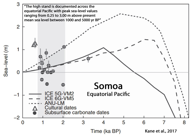
Kane et al., 2017 The high stand is documented across the equatorial Pacific with peak sea-level values ranging from 0.25 to 3.00 m above present mean sea level (MSL) between 1000 and 5000 yr BP (Fletcher and Jones, 1996; Grossman et al., 1998; Dickinson, 2003; Woodroffe et al., 2012). Woodroffe et al. (2012) argues that Holocene sea-level oscillations of a meter or greater are likely to have been produced by local rather than global processes.
Meltzner et al., 2017 Half-metre sea-level fluctuations on centennial timescales from mid-Holocene corals of Southeast Asia … RSL [relative sea level] history between 6850 and 6500 cal years BP that includes two 0.6 m fluctuations, with rates of RSL change reaching 13±4 mm per year. … Here RSL rose to an initial peak of +1.9 m [above present] at 6,720 cal years BP, then fell rapidly to a lowstand of +1.3 m, remaining at about that level for ∼100 years, before rising to a second peak at +1.7 m shortly after 6,550 cal years BP. Around 6,480 cal years BP, RSL appears to have fallen again to +1.3 m before rising to a third peak at +1.6 m or higher. … The peak rate of RSL rise, averaged over a 20-year running time window over the period of study (∼6,850–6,500 cal years BP), is +9.6±4.2 mm per year (2σ); the peak rate of RSL fall is −12.6±4.2 mm per year. … To put the ∼0.6 m mid-Holocene fluctuations in context, annual mean sea level in some modern tide-gauge records is seen to change by as much as 0.2–0.3 m on interannual timescales, and the interannual s.d. of sea surface height between 1979 and 2013 approached 0.1 m in some portions of the western Pacific. The central dome of each microatoll grew during a period when RSL was high; RSL then fell rapidly, killing the upper portions of the corals; RSL then stabilized at a lower elevation, forming a series of low concentric annuli ∼0.6 m higher than present-day analogues; RSL [relative sea level] then rose ∼0.6 m in less than a century, allowing the coral to grow upward to 1.2 m higher than modern living corals.
Khan et al., 2017 Only Suriname and Guyana [Caribbean] exhibited higher RSL [relative sea level] than present (82% probability), reaching a maximum height of ∼1 m [above present] at 5.2 ka [5,200 years ago]. … Because of meltwater input, the rates of RSL [relative sea level] change were highest during the early Holocene, with a maximum of 10.9 ± 0.6 m/ka [1.09 meters per century] in Suriname and Guyana and minimum of 7.4 ± 0.7 m/ka [0.74 meters per century] in south Florida from 12 to 8 ka [12,000 to 8,000 years ago].
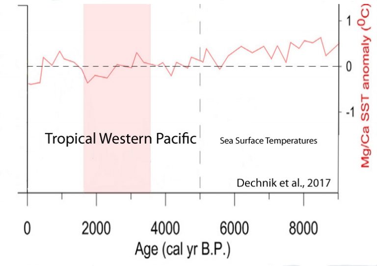
Dechnik et al., 2017 [I]t is generally accepted that relative sea level reached a maximum of 1–1.5 m above present mean sea level (pmsl) by ~7 ka [7,000 years ago] (Lewis et al., 2013) … Over the last few decades, the global decline of modern reefs has been linked to environmental and climatic changes in response to anthropogenic activities. However, recent geological and ecological research on fossil reefs in the Great Barrier Reef (GBR) and wider Indo-Pacific identified intervals of significant reef “turn-off” in response to natural environmental forces earlier in their development during the mid- to late Holocene. … Increased upwelling, turbidity and cyclone activity in response to increased sea-surface temperature (SST’s), precipitation and El-Nino Southern Oscillation variability have been ruled out as possible mechanisms of reef turn-off for the mid-outer platform reefs. Rather, a fall (~0.5 m) in relative sea level at 4–3.5 ka is the most likely explanation for why reefs in the northern and southern regions turned off during this time. … Similar hiatuses in Holocene reef growth were identified in Japan from about 5.9 to 5.8 ka, 4.4 to 4.0 ka and from 3.3 to 3.2 ka. They were attributed to oscillating sea level and relatively cold sea-surface temperatures.
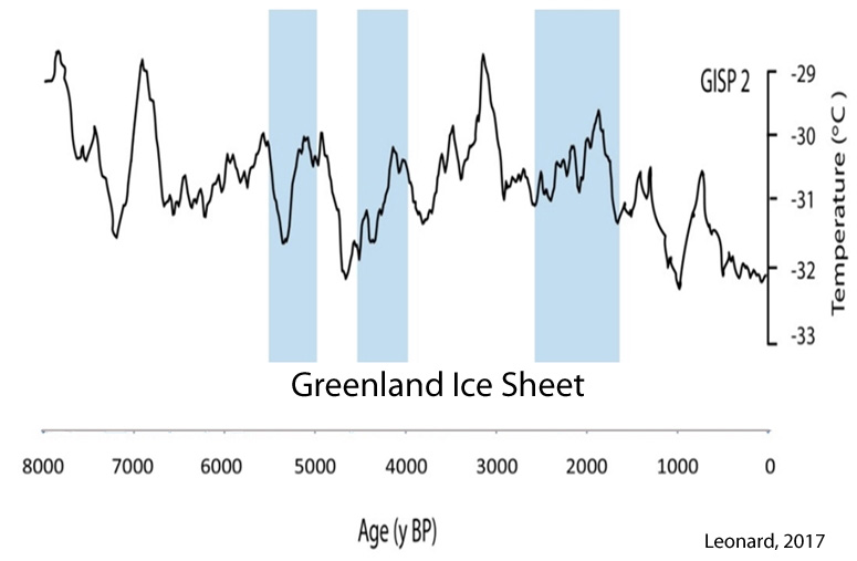
Leonard, 2017 The resultant palaeo-sea-level reconstruction revealed a rapid lowering of RSL of at least 0.4 m from 5500 to 5300 yBP following a RSL [relative sea level] highstand of ~0.75 m above present from ~6500 to 5500 yBP. RSL then returned to higher levels before a 2000-yr hiatus in reef flat corals after 4600 yBP. The RSL oscillations at 5500 yBP and 4600 yBP coincide with both substantial reduction in reef accretion and wide spread reef “turn-off”, respectively, thereby suggesting that oscillating sea level was the primary driver of reef shut down on the GBR.
Guo et al., 2017 The upper 250 meter-long sediment core of Site U1391 (1085 m water depth) retrieved from the Portuguese margin in the Northeast Atlantic Ocean was adopted for the benthic foraminiferal analyses to disclose the variations in Mediterranean Outflow Water (MOW) intensity over the last ~ 0.9 Ma [900,00 years]. The strongest MOW [Mediterranean Outflow Water] intensity during MIS 11 [400,000 years ago] confirms the climatic influence of waving sea level on the MOW current by its +20 m high-stand above the present sea level.
Cronin et al., 2017 Rates and patterns of global sea level rise (SLR) following the last glacial maximum (LGM) are known from radiometric ages on coral reefs from Barbados, Tahiti, New Guinea, and the Indian Ocean, as well as sediment records from the Sunda Shelf and elsewhere. … Lambeck et al. (2014) estimate mean global rates during the main deglaciation phase of 16.5 to 8.2 kiloannum (ka) [16,500 to 8,200 years ago] at 12 mm yr−1 [+1.2 meters per century] with more rapid SLR [sea level rise] rates (∼ 40 mm yr−1) [+4 meters per century] during meltwater pulse 1A ∼ 14.5–14.0 ka [14,500 to 14,000 years ago].
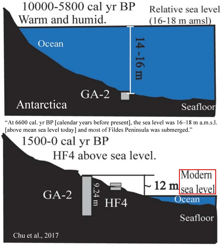
Chu et al., 2017 During 10 000–5800 cal. yr BP, Fildes Peninsula was warm and humid, grounded glaciers retreated and icefree regions were formed. At 6600 cal. yr BP, the sea level was 16–18 m a.m.s.l. [above mean sea level today] and most of Fildes Peninsula was submerged.
Miklavič et al., 2017 Holocene relative sea level history from phreatic overgrowths on speleothems (POS) on Minami Daito Island, Northern Philippine Sea… The results show that SL [sea level] reached its Holocene maximum between ca. 5.1 and 4.6 ka cal BP [4,600 to 5,100 years ago], after which it remained more or less stable till the present day, with a possible minor sea-level drawdown of ca. 30–35 cm…. The mid Holocene highstand is commonly assumed to have been ca. 3 m above the modern SL [sea level], although the observed heights range between +0.5 m and +4 m.
Abdul et al., 2017 We find that sea level tracked the climate oscillations remarkably well. Sea-level rise was fast in the early Allerød (25 mm yr-1), but decreased smoothly into the Younger Dryas (7 mm yr-1) when the rate plateaued to <4 mm yr-1here termed a sea-level “slow stand”. No evidence was found indicating a jump in sea level at the beginning of the Younger Dryas as proposed by some researchers. Following the “slow-stand”, the rate of sea-level rise accelerated rapidly, producing the 14 ± 2 m sea-level jump known as MWP-1B; occurred between 11.45 and 11.1 kyr BP with peak sea-level rise reaching 40 mm yr-1 [+4 meters per century].
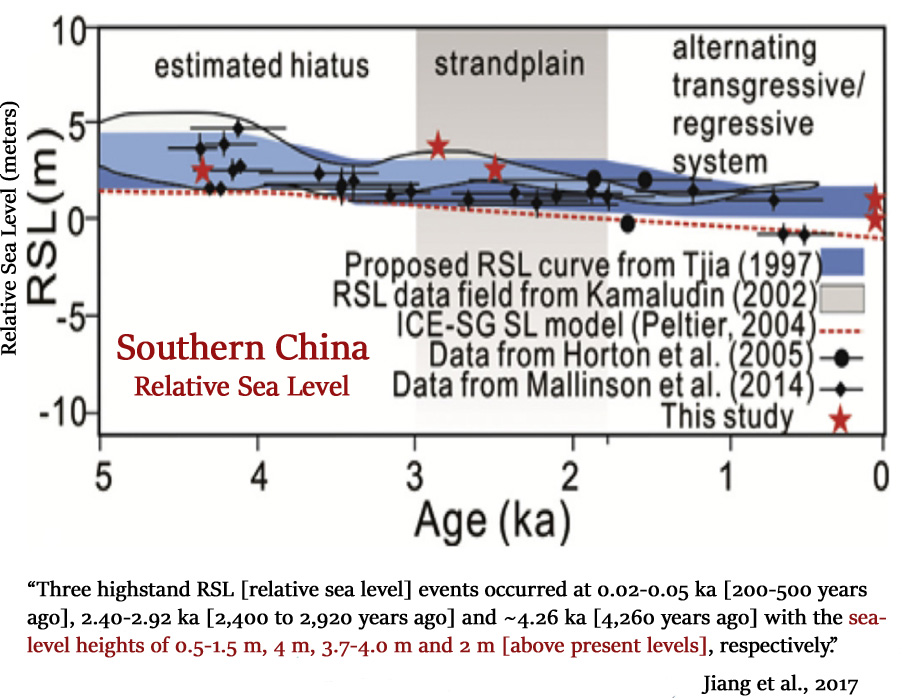
Jiang et al., 2017 [T]hree coastal sediments with 4 m, 3.7 m, and 2 m higher than present sea-level were deposited at 2.40 ± 0.05 ka, 2.92 ± 0.17 ka, and 4.26 ± 0.10 ka, respectively [2,400, 2,920, and 4,260 years before present], which indicate that the height of highstand relative sea-level are higher than both mean global sea-level eustacy and those records offshore southern China. … In conclusion, a beach ridge and two marine terraces sediments have been dated at eastern Hainan Island. They were well bleached and can be taken as good indicators of paleo-RSL [relative sea level] highstand records of late Holocene. Three highstand RSL [relative sea level] events occurred at 0.02-0.05 ka [200-500 years ago], 2.40-2.92 ka [2,400 to 2,920 years ago] and ~4.26 ka [4,260 years ago] with the sea-level heights of 0.5-1.5 m, 4 m, 3.7-4.0 m and 2 m [above present levels], respectively. The height of highstand RSLs are higher than both mean global sea-level euastacy and those of offshore southern China.
No Net Warming During 20th (21st) Century (12)
Zywiec et al., 2017
Flannery et al., 2017 The early part of the reconstruction (1733–1850) coincides with the end of the Little Ice Age, and exhibits 3 of the 4 coolest decadal excursions in the record. However, the mean SST estimate from that interval during the LIA is not significantly different from the late 20th Century SST mean. The most prominent cooling event in the 20th Century is a decade centered around 1965. This corresponds to a basin-wide cooling in the North Atlantic and cool phase of the AMO.

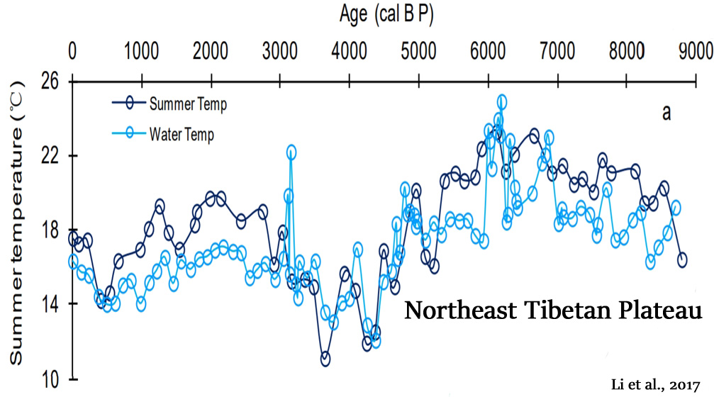
Li et al., 2017
Lan et al., 2017 Here, we present a new reconstruction of the temperature and precipitation change over the past two millennia based on grain size of a welldated glacial lake sediment core in the central of southern Tianshan Mountains. The results show that the glacial lake catchment has experienced cold-wet climate conditions during the Dark Age Cold Period (~300-600 AD; DACP) and the Little Ice Age (~1300-1870 AD; LIA), whereas warm-dry conditions during the Medieval Warm Period (~700-1270 AD; MWP). … The results show that the centennial HCA [High Central Asia] temperature changes not only significantly correlate with those in China (Yang et al., 2002a) and northwestern China (He et al., 2013), but also with those in Northern Hemisphere (Moberg et al., 2005; Ljungqvist, 2010), implying that the centennial HCA [High Central Asia] temperature changes may have similar driving forces with those in Northern Hemisphere at least over the past two millennia, like solar forcing (Bond et al., 2001; Gray et al., 2010; Moffa-Sanchez et al., 2014) and volcanic eruption (Schurer et al., 2014; Sigl et al., 2015; Stoffel et al., 2015), etc.
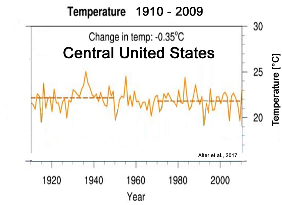
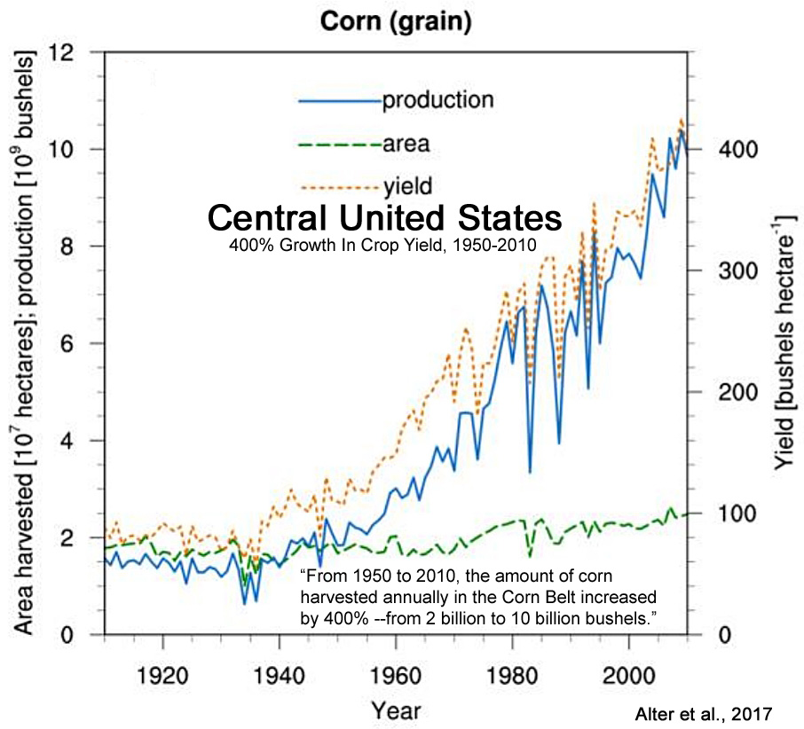
Alter et al., 2017 In the central United States … observational data indicate that rainfall increased, surface air temperature decreased, and surface humidity increased during the summer over the course of the 20th century concurrently with increases in both agricultural production and global GHG emissions. … Results of both regional climate model simulations and observational analyses suggest that much of the observed rainfall increase – as well as the decrease in temperature and increase in humidity – is attributable to agricultural intensification in the central United States, with natural variability and GHG emissions playing secondary roles. Thus, we conclude that 20th-century land-use changes contributed more to forcing observed regional climate change during the summer in the central United States than increasing GHG emissions. … From 1910- 1949 (pre-agricultural development, pre-DEV) to 1970-2009 (full agricultural development, full-DEV), the central United States experienced large-scale increases in rainfall of up to 35% and decreases in surface air temperature of up to 1°C during the boreal summer months of July and August … which conflicts with expectations from climate change projections for the end of the 21st century (i.e., warming and decreasing rainfall) (Melillo et al., 2014). … [T]he CMIP5 [climate model] results instead show an increase in temperature and a much subdued increase in specific humidity, which may be due to GHG-induced warming and subsequent increases in the water vapor holding capacity of the atmosphere, respectively. Thus, it seems that GHG emissions do not contribute greatly to the regional changes in summer climate that have been observed in the central United States. … Over the last century, the world has experienced unprecedented growth in cropland area and productivity (Ramankutty & Foley, 1999; Pielke et al., 2011). As part of this expansive agricultural development, the Corn Belt of the central United States – one of the most productive agricultural areas in the world (Guanter et al., 2014; Mueller et al., 2016) – experienced major increases in both corn and soybean production. For example, from 1950 to 2010, the amount of corn harvested annually in the Corn Belt increased by 400%, from 2 billion to 10 billion bushels (NASS, 2016).
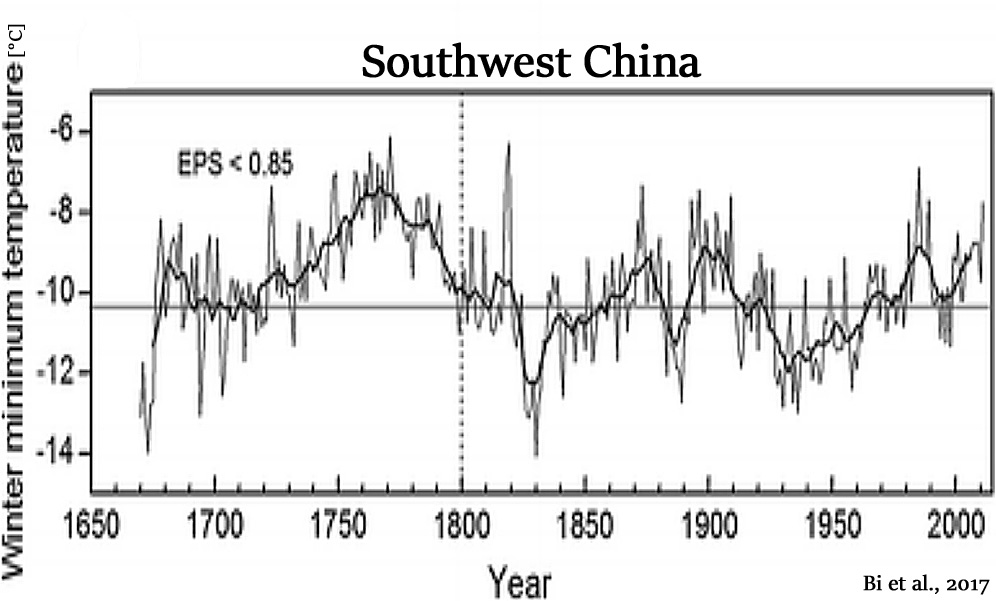
Bi et al., 2017 [T]he MWT [minimum winter temperature] values and rate of warming over the past seven decades [southwest China] did not exceed those found in the reconstructed temperature data for the past 211 years. … Larger scale climate oscillations of the Western Pacific and Northern Indian Ocean as well as the North Atlantic Oscillation probably influenced the region’s temperature in the past.
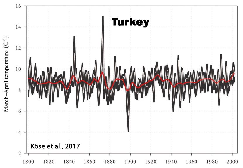
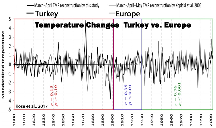
Köse et al., 2017 The reconstruction is punctuated by a temperature increase during the 20th century; yet extreme cold and warm events during the 19th century seem to eclipse conditions during the 20th century. We found significant correlations between our March–April spring temperature reconstruction and existing gridded spring temperature reconstructions for Europe over Turkey and southeastern Europe. … During the last 200 years, our reconstruction suggests that the coldest year was 1898 and the warmest year was 1873. The reconstructed extreme events also coincided with accounts from historical records. … Further, the warming trends seen in our record agrees with data presented by Turkes and Sumer (2004), of which they attributed [20th century warming] to increased urbanization in Turkey. Considering long-term changes in spring temperatures, the 19th century was characterized by more high-frequency fluctuations compared to the 20th century, which was defined by more gradual changes and includes the beginning of decreased DTRs [diurnal temperature ranges] in the region (Turkes and Sumer, 2004).
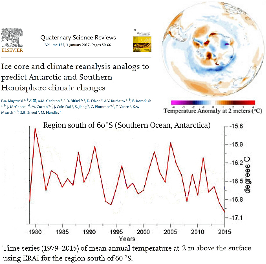
Mayewski et al., 2017
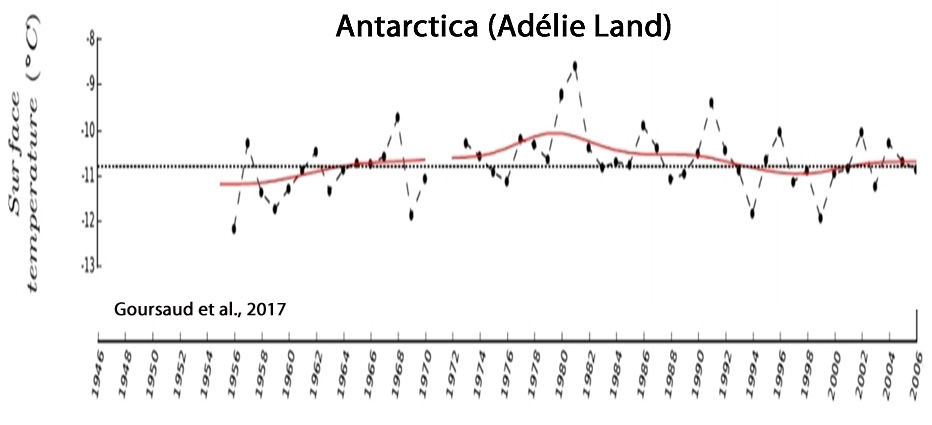
Goursaud et al., 2017
Imada et al., 2017 Since the late 1990s, land surface temperatures over Japan have increased during the summer and autumn, while global mean temperatures have not risen in this duration (i.e., the global warming hiatus). In contrast, winter and spring temperatures in Japan have decreased.
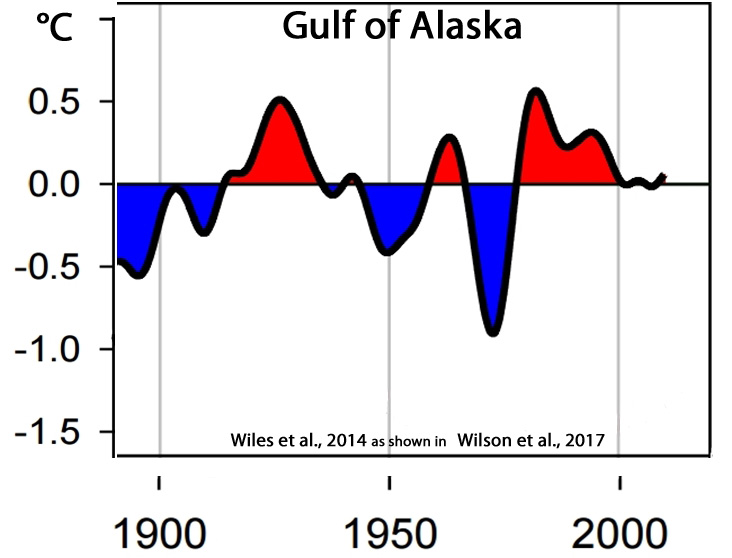
Wilson et al., 2017

Fernández-Fernández et al., 2017 The abrupt climatic transition of the early 20th century and the 25-year warm period 1925–1950 triggered the main retreat and volume loss of these glaciers since the end of the ‘Little Ice Age’. Meanwhile, cooling during the 1960s, 1970s and 1980s altered the trend, with advances of the glacier snouts. Between the ‘Little Ice Age’ and the present day, the mean annual air temperature and mean ablation season air temperature increased by 1.9°C and 1.5°C, respectively, leading to a 40–50 m rise in the equilibrium line altitude (ELA) of the glaciers during this period. … The retreat rate intensified in the period 2000–2005 compared with 1994–2000, but did not reach the rates recorded before 1946. … In the second half of the 20th century, the retreat decelerated considerably, reflected in the lowest values around 1985 (5.2 m yr−1) and a trend shift in 1994, with an advance observed in Gljúfurárjökull. The trend then altered again and Gljúfurárjökull retreated in the years 1994–2005. … During the period 1898–1946, the snout of Gljúfurárjökull retreated 635 m, almost two-thirds of the total distance from the LIA maximum (1898–1903) to 2005, at an average rate of 13.2 m yr−1. … The trend in Western Tungnahryggsjökull during the first half of the 20th century was a more rapid retreat, showing the highest average rates of the whole period (19.5 m yr−1). By 1946, this glacier had retreated almost 90% of the total recorded between the LIA maximum (1868) and 2005. … Just as in the glaciers described above, the retreat of the Eastern Tungnahryggsjökull from its LIA position was more intense during the first half of the 20th century, and in 1946 its snout was only 200 m from its current position. … The 2000 aerial photograph shows that an advance of at least 41 m had taken place since 1985. Nevertheless, between 2000 and 2005, the snout retreated 17 m, even more slowly than Western Tungnahryggsjökull. [Between 1985 and 2005, the Eastern Tungnahryggsjökull glacier did not retreat, but instead advanced by a net total of 24 meters.]

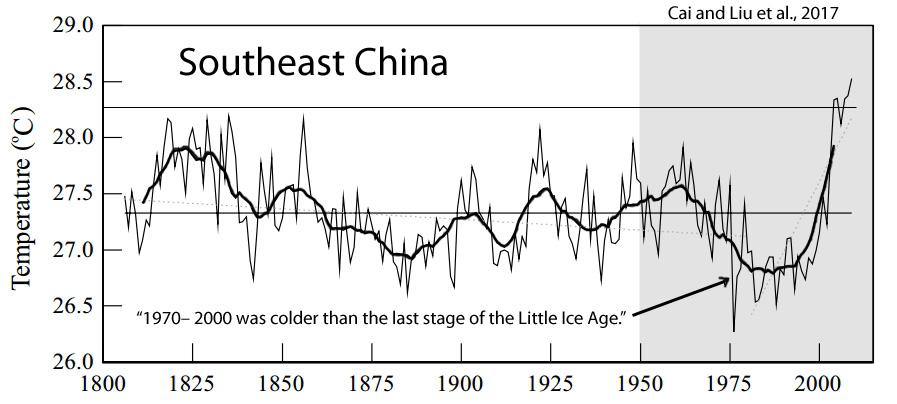
Cai and Liu et al., 2017 2003– 2009 was the warmest period in the reconstruction. 1970– 2000 was colder than the last stage of the Little Ice Age (LIA).
Warmer Past/Non-Hockey Stick Reconstructions (60)
![]()
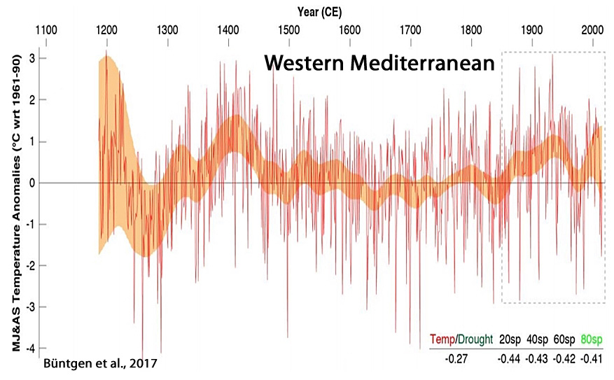
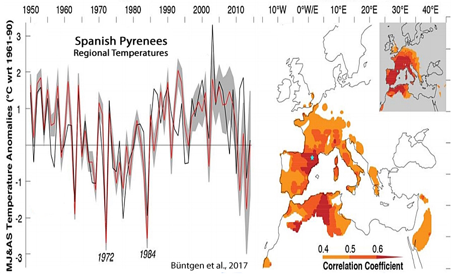
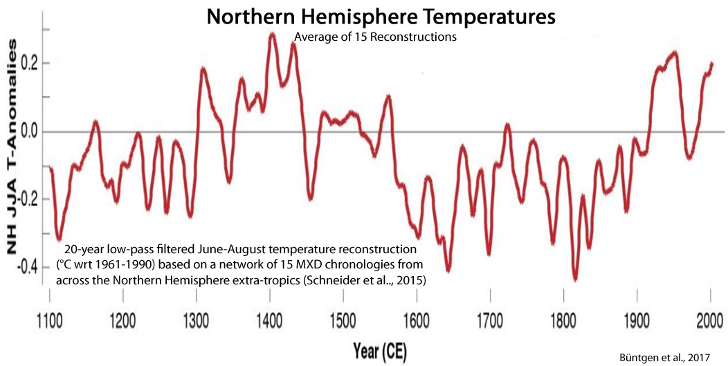
Büntgen et al., 2017 Spanning the period 1186-2014 CE, the new reconstruction reveals overall warmer conditions around 1200 and 1400, and again after ~1850. The coldest reconstructed summer in 1258 (-4.4°C wrt 1961-1990) followed the largest known volcanic eruption of the CE. The 20th century is characterized by pronounced summer cooling in the 1970s, subsequently rising temperatures until 2003, and a slowdown of warming afterwards. Little agreement is found with climate model simulations that consistently overestimate recent summer warming and underestimate pre-industrial temperature changes. … [W]hen it comes to disentangling natural variability from anthropogenically affected variability the vast majority of the instrumental record may be biased. … Although the causes of the recently measured slowdown in global and regional warming during the last decade are still debated (Karl et al. 2015; Fyfe et al. 2016), our study provides the first long-term proxy evidence for this temperature decline over the western Mediterranean basin. This finding is in line with local, regional and sub-continental meteorological observations, and consistent with the observations by Gleisner et al. (2015) that the post-2003 pause in rising mean surface temperatures is most strongly expressed at mid-latitudes. … The reconstructed long-term variability exceeds the pre-industrial multi-decadal to centennial variability in four state-of-the-art climate model simulations. This mismatch between the proxy reconstructions and the four model simulations is in line with a general tendency of state-of-the-art climate model simulations to underestimate the amplitude of reconstructed natural low-frequency temperature variability during the last millennium (Bothe et al. 2013; Fernández-Donado et al. 2013; Phipps et al. 2013; Luterbacher et al. 2016; Ljungqvist et al. 2012). Such disagreement might indicate that the role of internal unforced variability is greater than expected (Goosse 2017; Matsikaris et al. 2016), and/or that the climate sensitivity to the prescribed forcings needs adjustment. … [S]tate-of-the-art climate models are usually driven by a relatively dampened amplitude of long-term changes in solar activity (Schmidt et al. 2011,2012).
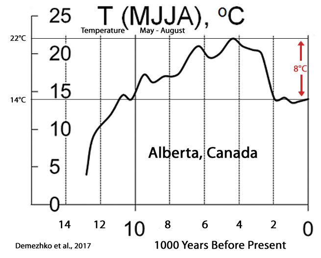
Demezhko et al., 2017 Temperature and heat flux changes at the base of Laurentide ice sheet inferred from geothermal data … The temperature curve reveals a sharp rise in the early Holocene (12−10-ka BP) and a relatively stable warm climate of interglacial, while the heat flux began to increase about 2 ka earlier, reached a maximum at the beginning of the Holocene, and then decreased. … GSTH [ground surface temperature histories] reconstructed under SD=0.02 W/(m K) reveals major climatic events of the last 100 ka including the Last Glacial Maximum around 20 ka BP with a minimum temperature −2.7°C, the Holocene Climatic Optimum around 5 ka BP with the maximal temperature+8.4°C, and subsequent cooling to the contemporary mean surface temperature +4°C. [Surface temperatures were 4.4°C higher than present 5,000 years ago]. … GST [ground surface temperature] and SHF [surface heat flux] histories differ substantially in shape and chronology. Heat flux changes ahead temperature changes by 500–1000 years. … These results (Fig. 4d) indicate an abrupt increase of summer (from May to August) temperatures between 12 and 10 ka BP, relative stabilization 10–7 ka BP, another increase after 7 ka BP, and rapid decline to modern values after 3 ka BP. … The amount of heat accumulated by the Earth in the last glacial cycle is a small fraction (<1%) of the heat released due to insolation changes. At the same time, the amount of heat spent on glacier melting is comparable with heat coming due to insolation.
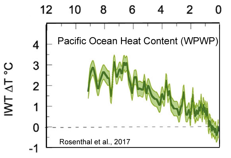
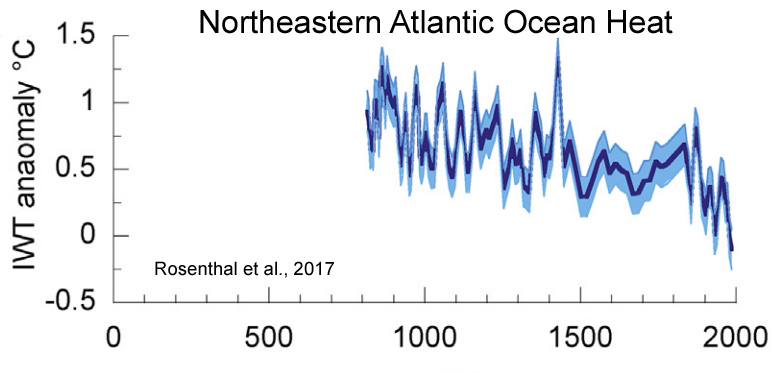
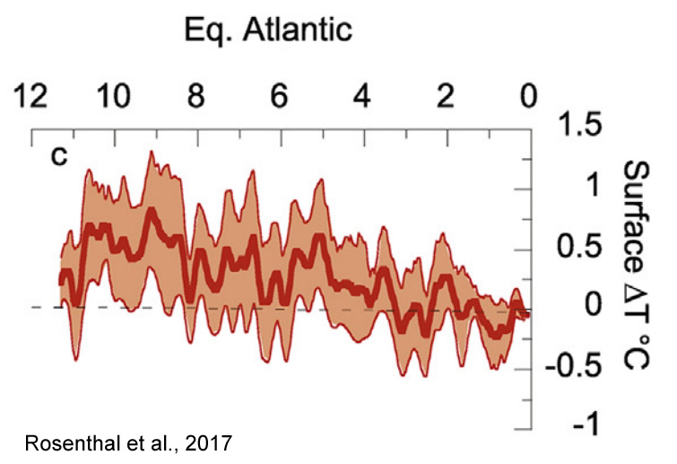
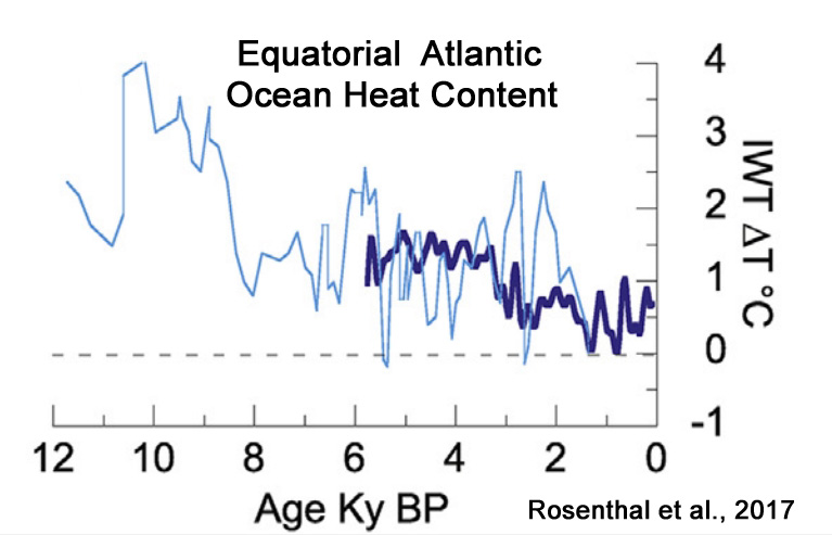
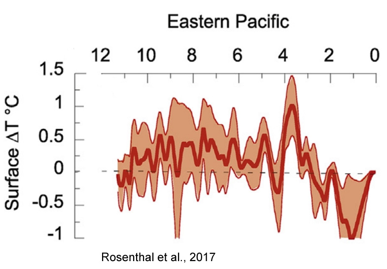
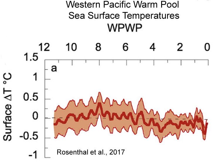
Rosenthal et al., 2017 Here we review proxy records of intermediate water temperatures from sediment cores and corals in the equatorial Pacific and northeastern Atlantic Oceans, spanning 10,000 years beyond the instrumental record. These records suggests that intermediate waters [0-700 m] were 1.5-2°C warmer during the Holocene Thermal Maximum than in the last century. Intermediate water masses cooled by 0.9°C from the Medieval Climate Anomaly to the Little Ice Age. These changes are significantly larger than the temperature anomalies documented in the instrumental record. The implied large perturbations in OHC and Earth’s energy budget are at odds with very small radiative forcing anomalies throughout the Holocene and Common Era. … The records suggest that dynamic processes provide an efficient mechanism to amplify small changes in insolation [surface solar radiation] into relatively large changes in OHC.
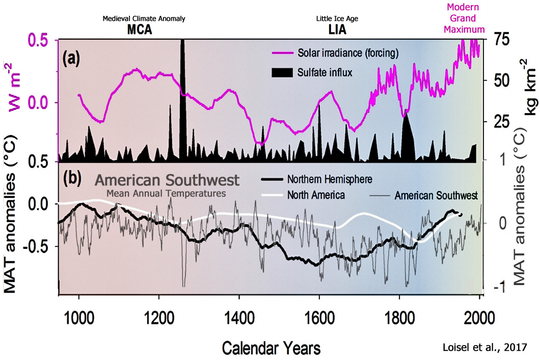
Loisel et al., 2017 The Medieval Climate Anomaly (MCA, ~950–1400 CE) is often used as an analog for 21stcentury hydroclimate because it represents a warm (and arid) period. The MCA appears related to general surface warming in the Northern Hemisphere, prolonged La Niña conditions, and a persistent positive North Atlantic Oscillation mode. It has been referred to as a stable time interval with ‘quiet’ conditions in regards to low perturbation by external radiative forcing. In this study, we demonstrate that the Little Ice Age (LIA, ~1400–1850 CE) might be more representative of future hydroclimatic variability than the conditions during the MCA megadroughts for the American Southwest, and thus provide a useful scenario for development of future water-resource management and drought and flood hazard mitigation strategies.
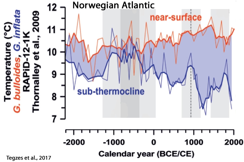
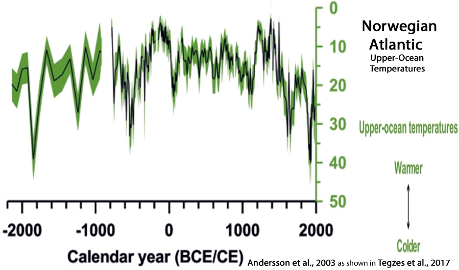
Tegzes et al., 2017 The objective of this study was to investigate northward oceanic heat transport in the NwASC [Norwegian Atlantic Slope Current] on longer, geologically meaningful time scales. To this end, we reconstructed variations in the strength of the NwASC over the late-Holocene using the sortable-silt method. We then analysed the statistical relationship between our palaeo-flow reconstructions and published upper-ocean hydrography proxy records from the same location on the mid-Norwegian Margin. Our sortable-silt time series show prominent multi-decadal to multi-centennial variability, but no clear long-term trend over the past 4200 years. … [O]ur findings indicate that variations in the strength of the main branch of the Atlantic Inflow may not necessarily translate into proportional changes in northward oceanic heat transport in the eastern Nordic Seas.
Guillet et al., 2017

Werner et al., 2017 During the MCA, the contrast between reconstructed summer temperatures over mid- and high-latitudes in Europe and the European/North Atlantic sector of the Arctic shows a very dynamic expression of the Arctic amplification, with leads and lags between continental and more marine and extreme latitude settings. While our analysis shows that the peak MCA [Medieval Climate Anomaly] summer temperatures were as high as in the late 20th and early 21st century, the spatial coherence of extreme years over the last decades seems unprecedented at least back until 750 CE. However, statistical testing could not provide conclusive support of the contemporary warming to supersede the peak of the MCA in terms of the pan-Arctic mean summer temperatures.

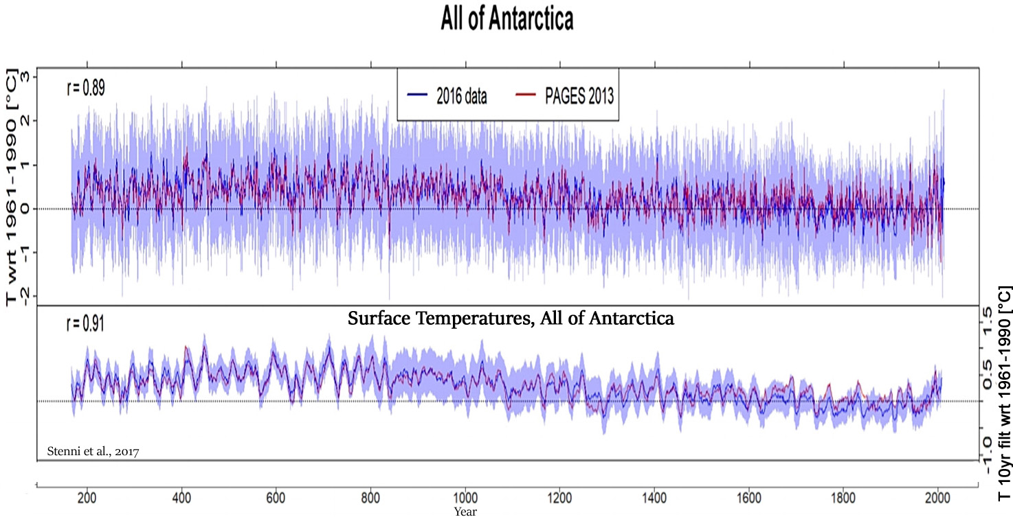
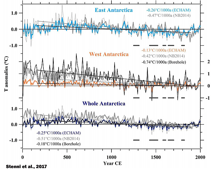
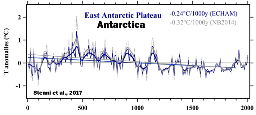
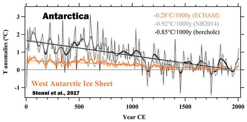
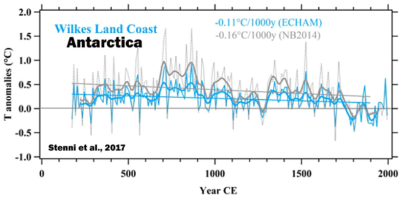
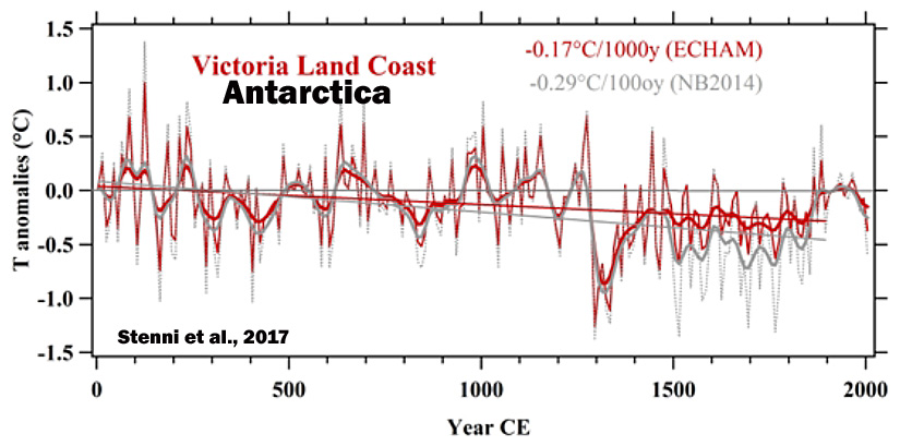
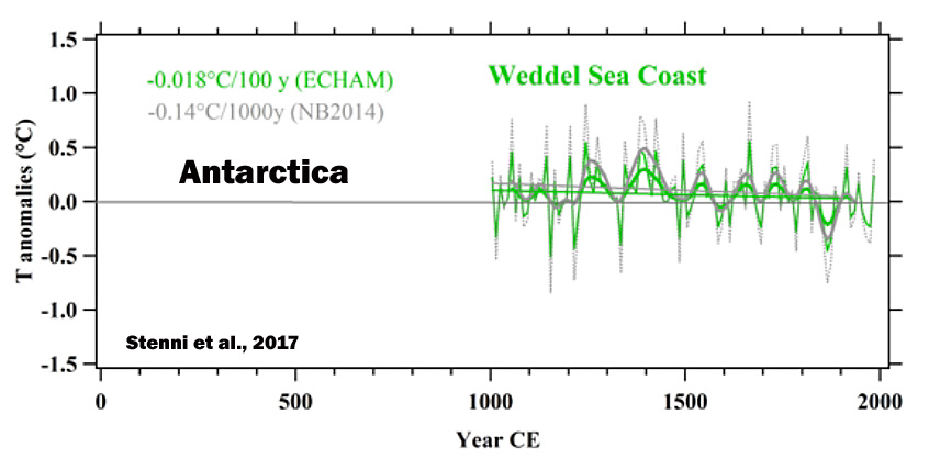
Stenni et al., 2017 Within this long-term cooling trend from 0-1900 CE we find that the warmest period occurs between 300 and 1000 CE, and the coldest interval from 1200 to 1900 CE. … A recent effort to characterize Antarctic and sub-Antarctic climate variability during the last 200 years also concluded that most of the trends observed since satellite climate monitoring began in 1979 CE cannot yet be distinguished from natural (unforced) climate variability (Jones et al., 2016), and are of the opposite sign [cooling, not warming] to those produced by most forced climate model simulations over the same post-1979 CE interval. … While changes in the SAM have been related to the human influence on stratospheric ozone and greenhouse gases (Thompson et al., 2011), major gaps remain in identifying the drivers of multi-centennial Antarctic climate variability. For instance, the influence of solar and volcanic forcing on Antarctic climate variability remains unclear. This is due to both the lack of observations and to the lack of confidence in climate model skill for the Antarctic region (Flato et al., 2013). … Our new continental scale reconstructions, based on the extended database, corroborates previously published findings for Antarctica from the PAGES2k Consortium (2013): (1) Temperatures over the Antarctic continent show an overall cooling trend during the period from 0 to 1900CE, which appears strongest in West Antarctica, and (2) no continent-scale warming of Antarctic temperature is evident in the last century.
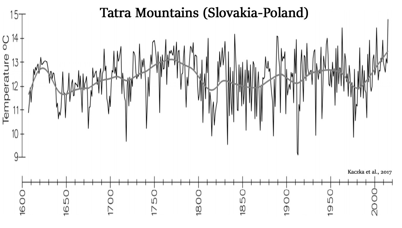
Kaczka et al., 2017
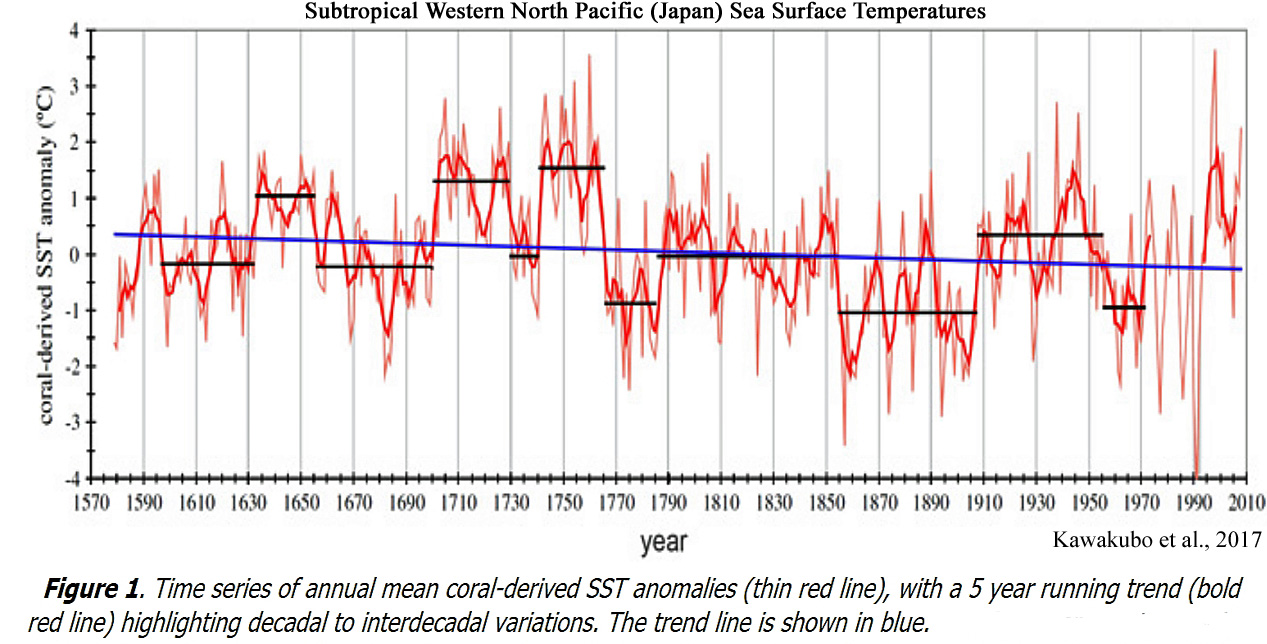
Kawakubo et al., 2017
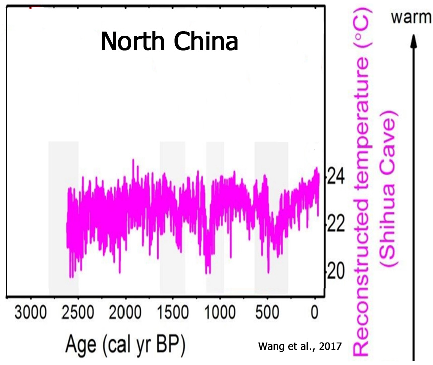
Wang et al., 2017 Our results show that: (1) the mean annual temperature (TANN) was relatively high from 4000-2700 cal yr BP, decreased gradually from 2700-1270 cal yr BP, and then fluctuated drastically during the last 1270 years. (2) A cold climatic event in the Era of Disunity, the Sui-Tang Warm Period (STWP), the Medieval Warm Period (MWP) and the Little Ice Age (LIA) can all be recognized in the paleotemperature record, as well as in many other temperature reconstructions in China.
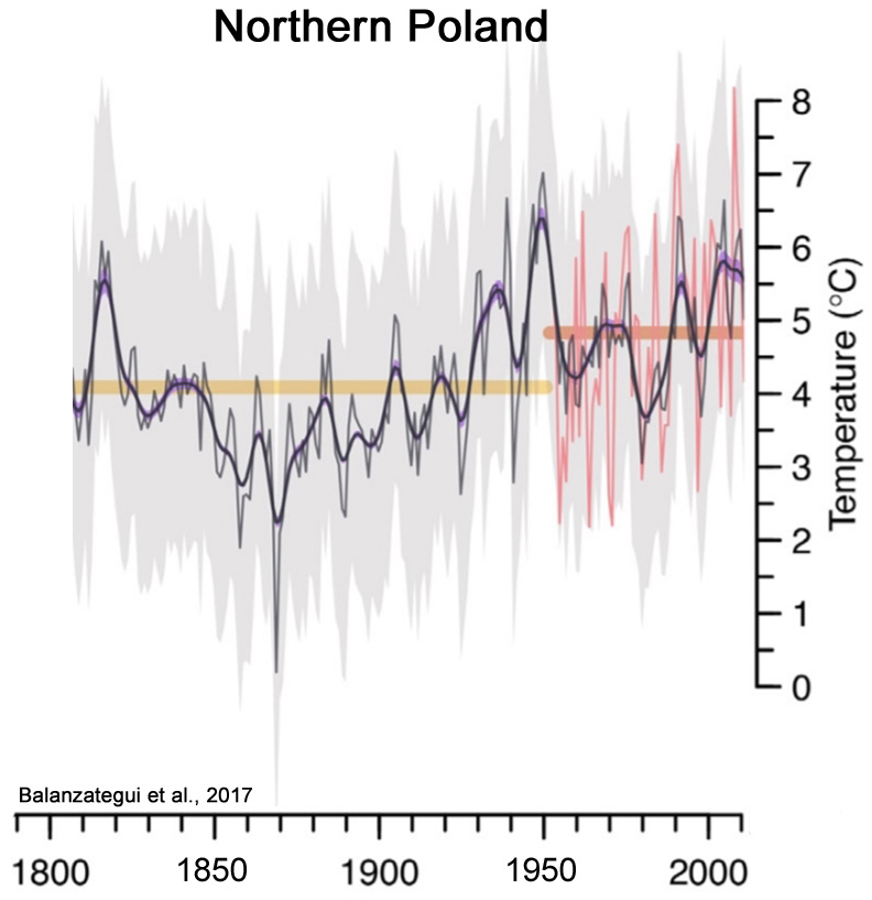
Balanzategui et al., 2017
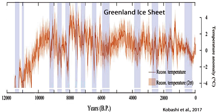
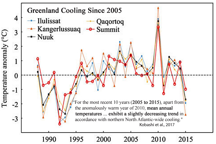
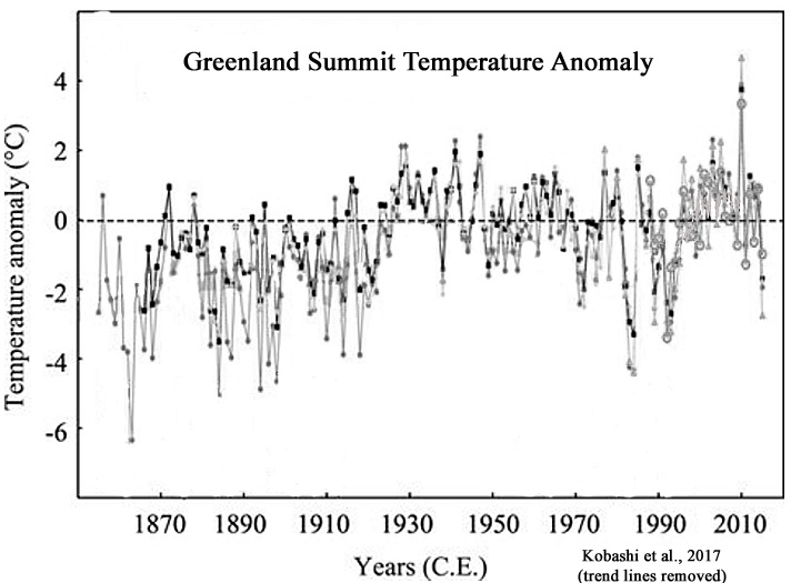
Kobashi et al., 2017 After the 8.2 ka event, Greenland temperature reached the Holocene thermal maximum with the warmest decades occurring during the Holocene (2.9 ± 1.4 °C warmer than the recent decades) at 7960 ± 30 years B.P. … For the most recent 10 years (2005 to 2015), apart from the anomalously warm year of 2010, mean annual temperatures at the Summit exhibit a slightly decreasing trend in accordance with northern North Atlantic-wide cooling. The Summit temperatures are well correlated with southwest coastal records (Ilulissat, Kangerlussuaq, Nuuk, and Qaqortoq).
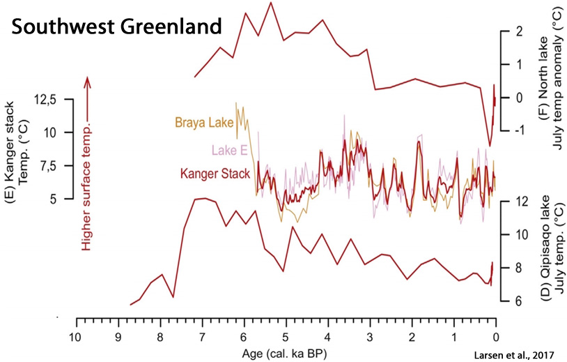
Larsen et al., 2017 [K]nowledge remains sparse of GICs [glaciers and ice caps] fluctuations in Greenland and whether they survived past warmer conditions than today, e.g. the Holocene Thermal Maximum (HTM) ~8-5 cal. ka BP and the Medieval Climate Anomaly (MCA) ~1200-950 C.E. Only a few available studies have provided continuous records of Holocene glacier fluctuations in east Greenland (Lowell et al., 2013; Levy et al., 2014; Balascio et al., 2015) and west Greenland (Schweinsberg et al., 2017). These records show that local GICs [glaciers and ice caps] were significantly reduced and most likely completely absent during the HTM [Holocene Thermal Maximum].
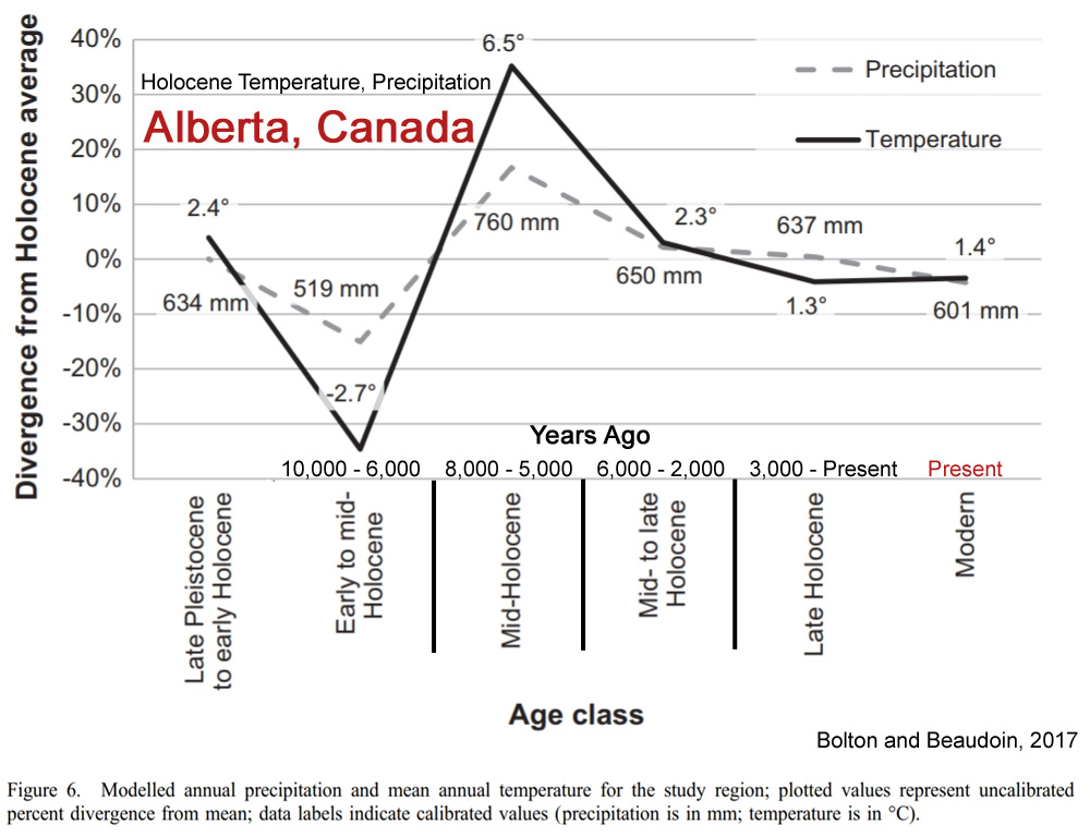
Bolton and Beaudoin, 2017 Major late Holocene fluctuations include intervals of warmer (e.g. Medieval Warm Period) and cooler (e.g. Little Ice Age) climate. … The modern period [21st century] had temperature and precipitation values which were about 4% less than the Holocene average (Figure 6).
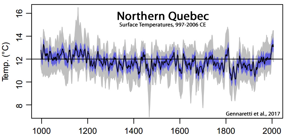
Gennaretti et al., 2017
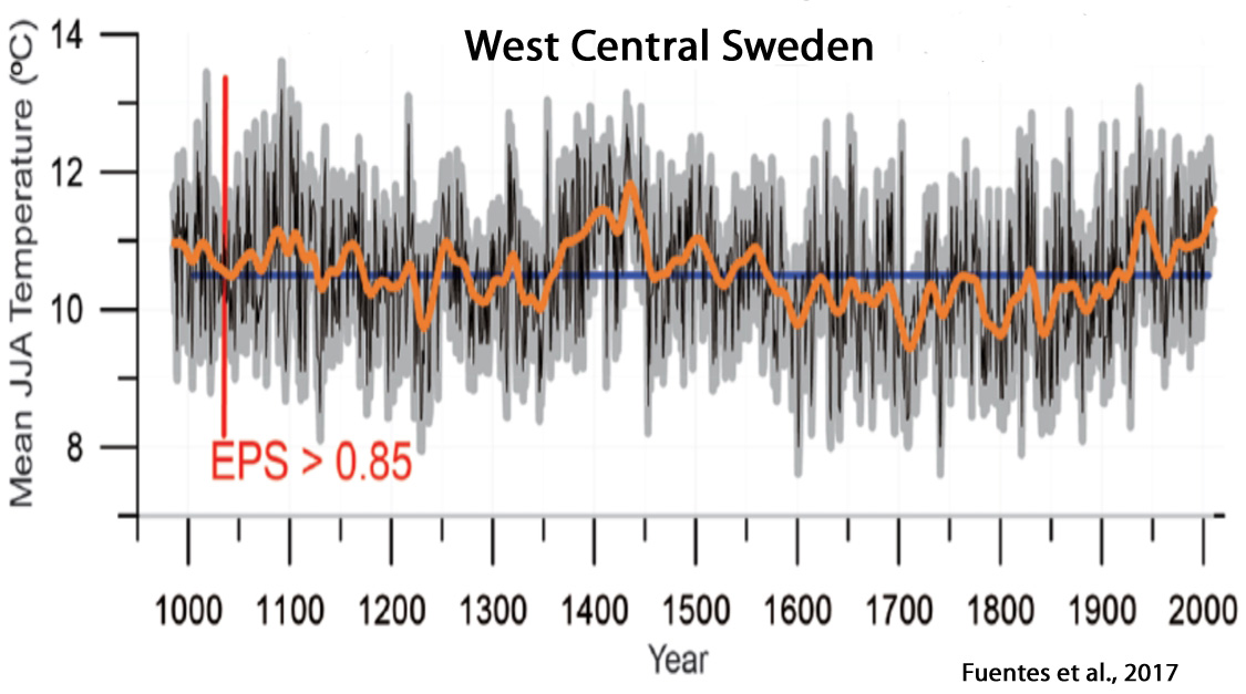
Fuentes et al., 2017 The summer (June through August) temperature reconstruction, extending back to 1038 CE, exhibits three warm periods in 1040–1190 CE, 1370–1570 CE and the 20th century and one extended cold period between 1570 and 1920 CE.
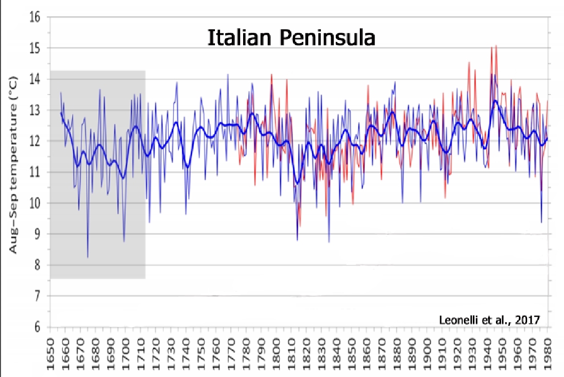
Leonelli et al., 2017
![]()
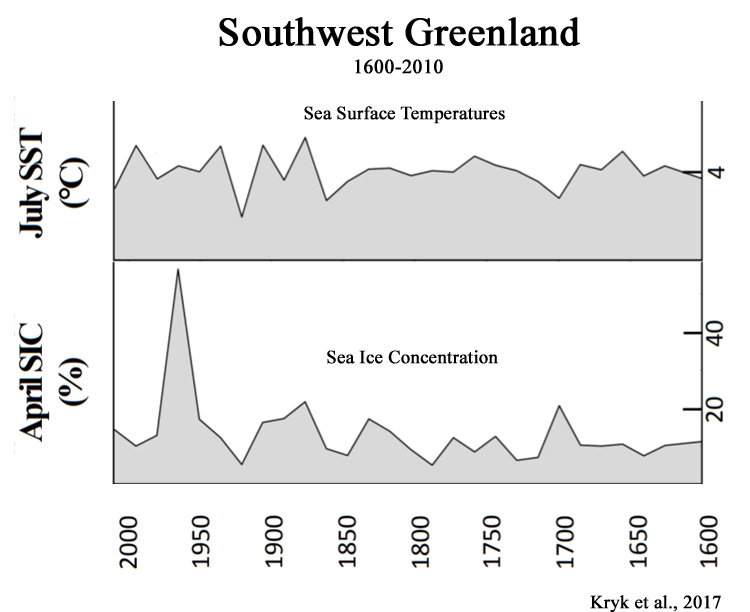
Kryk et al., 2017 Our study aims to investigate the oceanographic changes in SW Greenland over the past four centuries (1600-2010) based on high-resolution diatom record using both, qualitative and quantitative methods. July SST during last 400 years varied only slightly from a minimum of 2.9 to a maximum of 4.7 °C and total average of 4°C. 4°C is a typical surface water temperature in SW Greenland during summer. … The average April SIC was low (c. 13%) [during the 20th century], however a strong peak of 56.5% was recorded at 1965. This peak was accompanied by a clear drop in salinity (33.2 PSU).
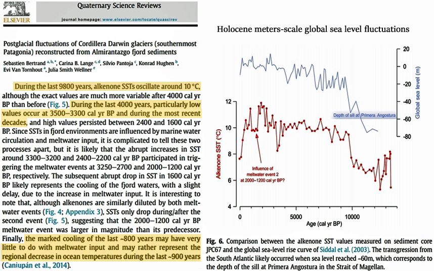
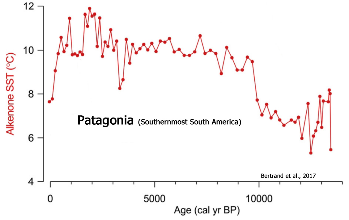
Bertrand et al., 2017 During the last 4000 years, particularly low [sea surface temperature] values occur at 3500-3300 cal yr BP and during the most recent decades, and high values persisted between 2400 and 1600 cal yr BP. … [I]t is likely that the abrupt increases in SST around 3300-3200 and 2400-2200 cal yr BP participated in triggering the meltwater events at 3250-2700 and 2000-1200 cal yr BP, respectively. … [T]he marked cooling of the last ~800 years may have very little to do with meltwater input and may rather represent the regional decrease in ocean temperatures during the last ~900 years (Caniupan et al., 2014).
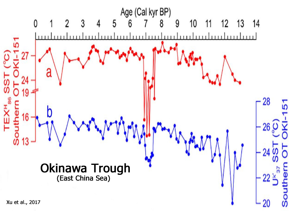
Xu et al., 2017 A significant drop in SSTs occurred at 7.6–6.9 kyr BP (centered on 7.3 kyr BP), indicating that the 7.3 kyr BP cold event was widely recorded in the Okinawa Trough. However, the TEXH 86-based SSTs dropped approximately 14 °C, and the amplitude of this SST drop was far greater than the one that occurred during the YD period.
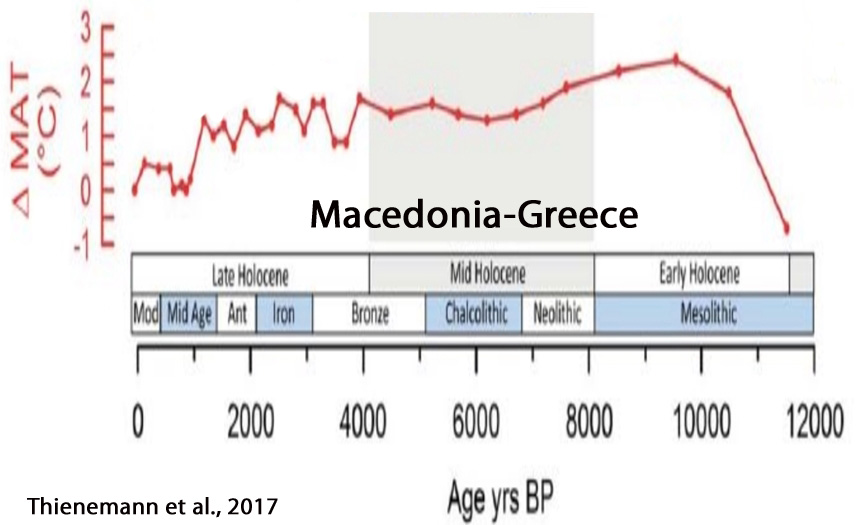
Thienemann, 2017
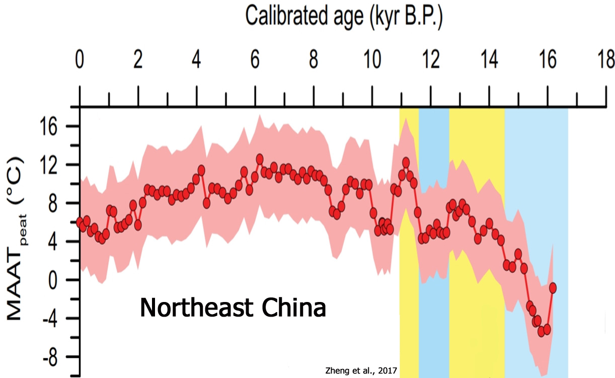
Zheng et al., 2017 From 11.5 to 10.7 ka [11,500 to 10,700 years ago], corresponding to the Preboreal event, MAATpeat indicates even higher [temperature] values, from 7.0 to 12 °C. MAATpeat continued to vary during the Holocene. From 10.7 to 6.0 ka, temperatures rose stepwise, with 2 cool events at 10.6–10.2 and 8.6 ka, before reaching maximum values of ~11 °C during the early Holocene from 8.0 to 6.0 ka. Following the early Holocene, temperatures at Hani gradually decreased to values of ~5 °C, close to the observed temperature at Hani across the past 60 yr (4–7.5 °C). [Modern temperatures are about 5-6°C colder than 6,000 to 8,000 years ago.]
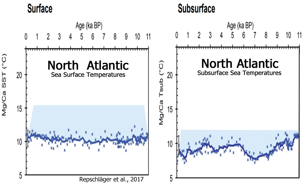
Repschläger et al., 2017 Shorter periodic climatic cycles, with average duration of about 1500 years, are observed in many Holocene climate records, and are superimposed on the long-term trend. The causes of these cycles are controversially discussed, with hypotheses ranging from meltwater pulses induced by variations in solar irradiance to internal ocean–ice–atmosphere feedback mechanisms or volcanism (e.g., Andrews and Giraudeau, 2003; Bond et al., 2001; Campbell et al., 1998; Schulz et al., 2004; Viau et al., 2006; Wanner, 2008). Due to the wide range of feedback mechanisms, involving northern hemispheric oceanic and atmospheric circulation, climate patterns with strong local differences are observed for the Holocene. Therefore, identification and understanding of the importance of the different driving forces and stabilizing mechanisms for the Holocene climate remains challenging.
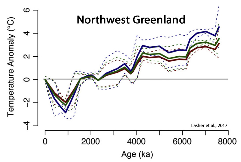
Lasher et al., 2017 This paper presents a multi proxy lake record of NW Greenland Holocene climate. … Summer temperatures (2.5–4 °C warmer than present) persisted until ∼4 ka [4,000 years ago] … Continual cooling after 4 ka led to coldest temperatures after 1.2 ka, with temperature anomalies 2-3°C below present. Approximately 1000 km to the south, a 2-3°C July temperature anomaly (relative to [warmer than] present) between 6 and 5 ka was reported based upon chironomid assemblages near Illulisat and Jakobshavn (Axford et al., 2013). Across Baffin Bay on northeastern Baffin Island, HTM summer temperatures were an estimated ~5°C warmer than the pre-industrial late Holocene and 3.5°C warmer than present, based upon chironomid assemblages (Axford et al., 2009; Thomas et al., 2007). … Following deglaciation, the GrIS [Greenland Ice Sheet] retreated behind its present margins (by as much as 20-60 km in some parts of Greenland) during the HTM [Holocene Thermal Maximum] (Larsen et al., 2015; Young and Briner, 2015).
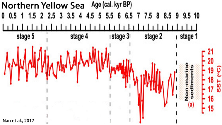
Nan et al., 2017
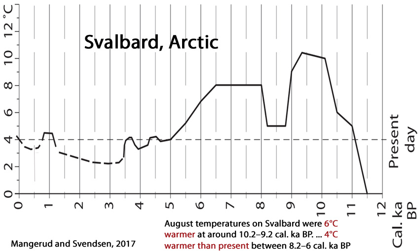
Mangerud and Svendsen, 2017 Shallow marine molluscs that are today extinct close to Svalbard, because of the cold climate, are found in deposits there dating to the early Holocene. The most warmth-demanding species found, Zirfaea crispata, currently has a northern limit 1000 km farther south, indicating that August temperatures on Svalbard were 6°C warmer at around 10.2–9.2 cal. ka BP, when this species lived there. … After 8.2 cal. ka, the climate around Svalbard warmed again, and although it did not reach the same peak in temperatures as prior to 9 ka, it was nevertheless some 4°C warmer than present between 8.2 and 6 cal. ka BP. Thereafter, a gradual cooling brought temperatures to the present level at about 4.5 cal. ka BP. The warm early-Holocene climate around Svalbard was driven primarily by higher insolation and greater influx of warm Atlantic Water, but feedback processes further influenced the regional climate.
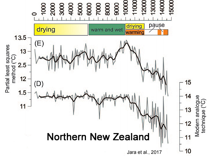
Jara et al., 2017
Lemmen and Lacourse, 2017 Between ~10,500 and 8000 cal year BP, inferred temperatures increase to ~16–18 °C, or up to ~3.7°C higher than inferred modern temperatures. This early Holocene warm period is followed by generally cooler inferred temperatures in the middle and late Holocene.
Browne et al., 2017
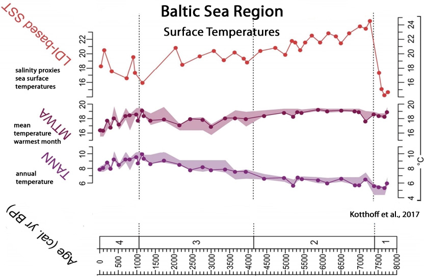
Kotthoff et al., 2017
Zhang et al., 2017 [S]ummer temperature variability at the QTP [Qinghai-Tibetan Plateau] responds rapidly to solar irradiance changes in the late Holocene.
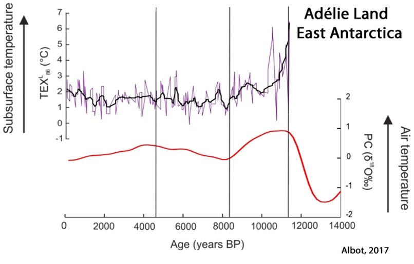
Albot, 2017 Growing paleoclimatic evidence suggests that the climatic signals of Medieval Warm Period and the Little Ice Age events can be detected around the world (Mayewski et al., 2004; Bertler et al., 2011). … [T]he causes for these events are still debated between changes in solar output, increased volcanic activity, shifts in zonal wind distribution, and changes in the meridional overturning circulation (Crowley, 2000; Hunt, 2006).
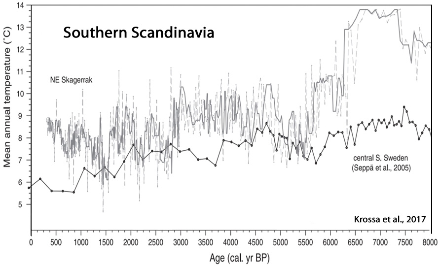
Krossa et al., 2017
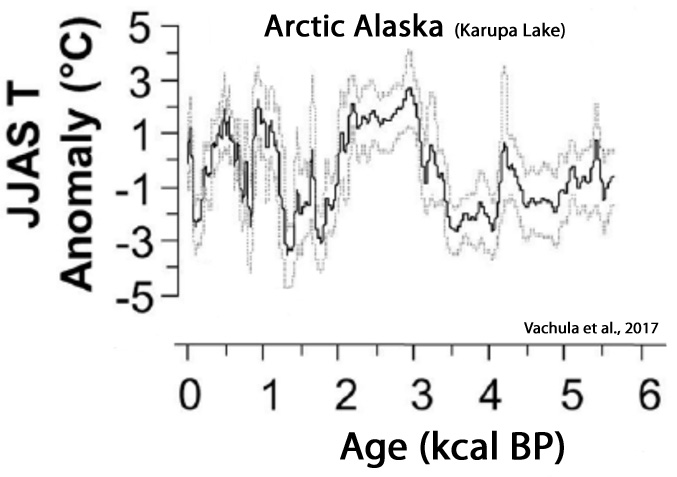
Vachula et al., 2017
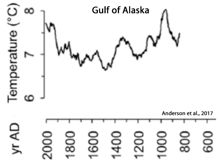
Anderson et al., 2017
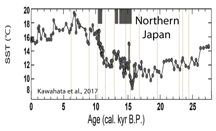
Kawahata et al., 2017 The SST [sea surface temperature] shows a broad maximum (~17.3 °C) in the mid-Holocene (5-7 cal kyr BP), which corresponds to the Jomon transgression. … The SST maximum continued for only a century and then the SST dropped by 3.5 °C [15.1 to 11.6 °C] within two centuries. Several peaks fluctuate by 2°C over a few centuries.
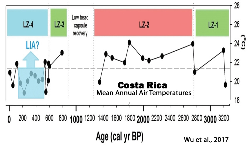
Wu et al., 2017 The existence of depressed MAAT [mean annual temperatures] (1.3°C lower than the 3200-year average) between 1480 CE and 1860 CE (470–90 cal. yr BP) may reflect the manifestation of the ‘Little Ice Age’ (LIA) in southern Costa Rica. Evidence of low-latitude cooling and drought during the ‘LIA’ has been documented at several sites in the circum-Caribbean and from the tropical Andes, where ice cores suggest marked cooling between 1400 CE and 1900 CE. Lake and marine records recovered from study sites in the southern hemisphere also indicate the occurrence of ‘LIA’ cooling. High atmospheric aerosol concentrations, resulting from several large volcanic eruptions and sea-ice/ocean feedbacks, have been implicated as the drivers responsible for the ‘LIA’. [Modern temperatures not significantly different than the LIA.]
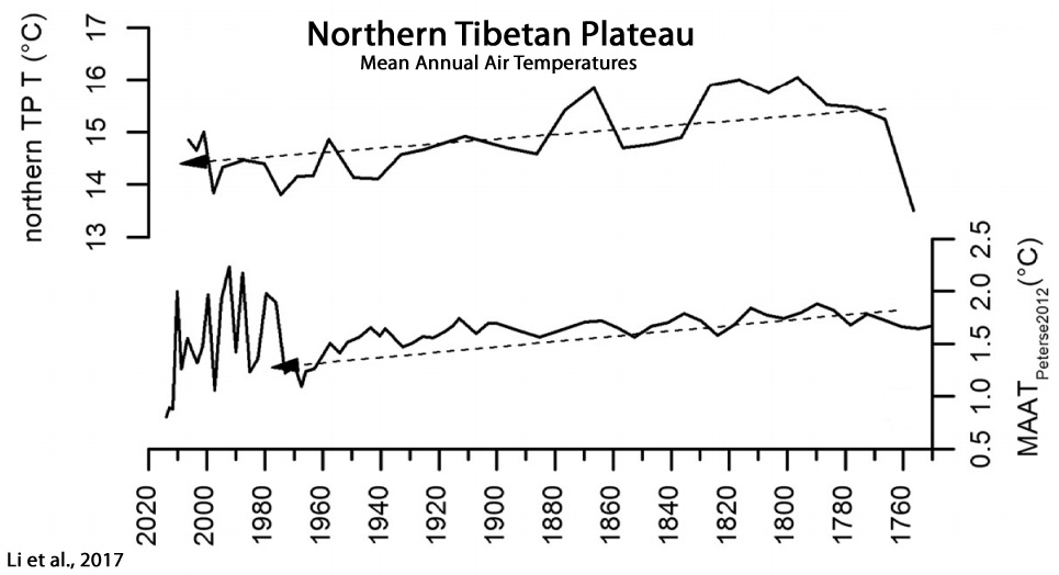
Li et al., 2017 Contrary to the often-documented warming trend over the past few centuries, but consistent with temperature record from the northern Tibetan Plateau, our data show a gradual decreasing trend of 0.3 °C in mean annual air temperature from 1750 to 1970 CE. This result suggests a gradual cooling trend in some high altitude regions over this interval, which could provide a new explanation for the observed decreasing Asian summer monsoon. In addition, our data indicate an abruptly increased interannual-to decadal-scale temperature variations of 0.8 – 2.2 °C after 1970 CE, in terms of both magnitude and frequency, indicating that the climate system in high altitude regions would become more unstable under current global warming.
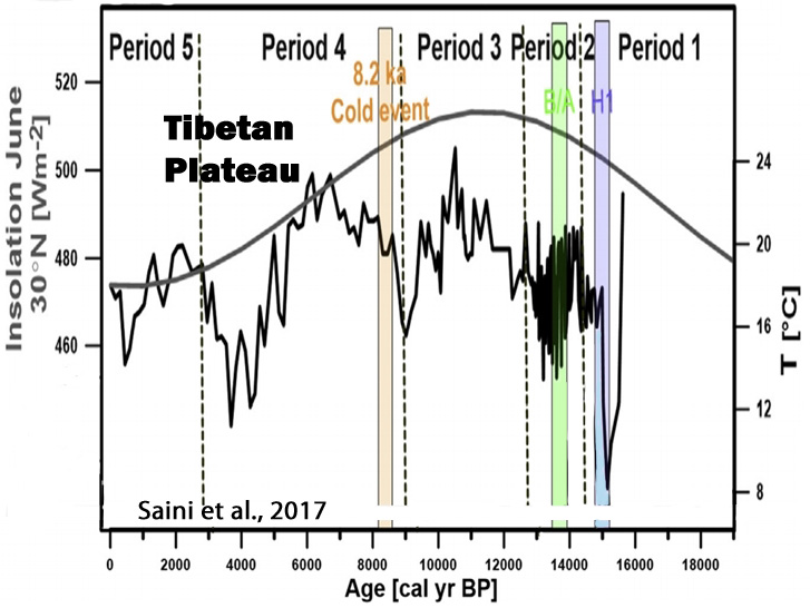
Saini et al., 2017
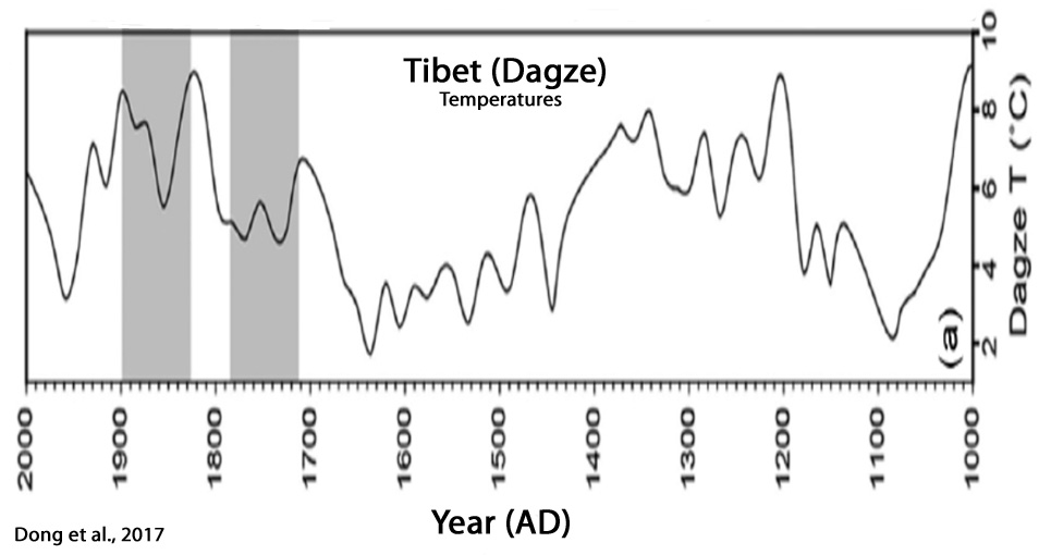
Dong et al., 2017
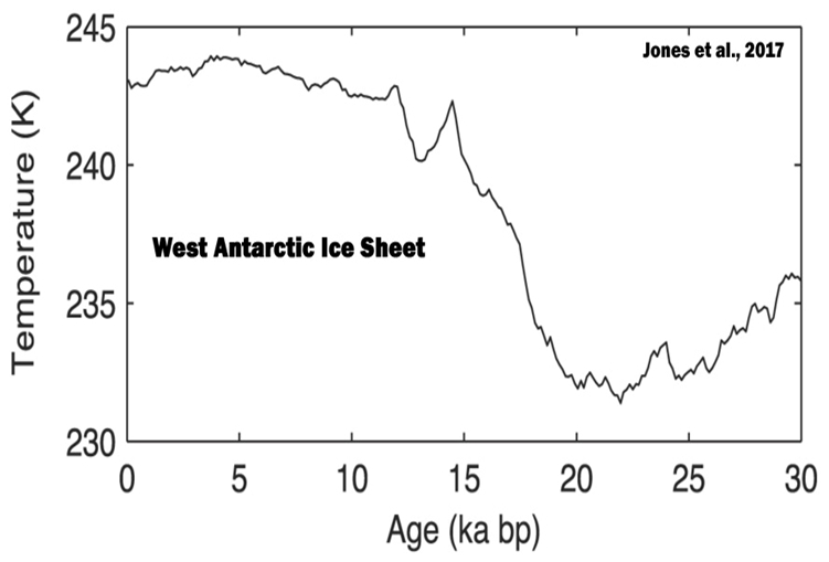
Jones et al., 2017
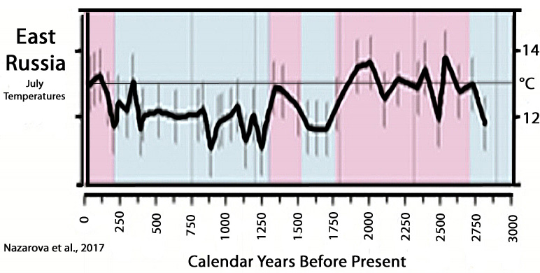
Nazarova et al., 2017 The application of transfer functions resulted in reconstructed T July fluctuations of approximately 3 °C over the last 2800 years. Low temperatures (11.0-12.0 °C) were reconstructed for the periods between ca 1700 and 1500 cal yr BP (corresponding to the Kofun cold stage) and between ca 1200 and 150 cal yr BP (partly corresponding to the Little Ice Age [LIA]). Warm periods (modern T[emperatures] July or higher) were reconstructed for the periods between ca 2700 and 1800 cal yr BP, 1500 and 1300 cal yr BP and after 150 cal yr BP.
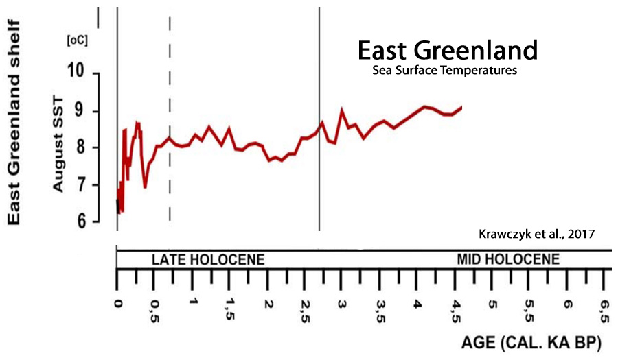
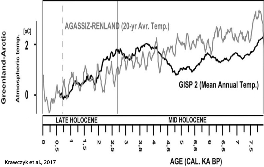
Krawczyk et al., 2017
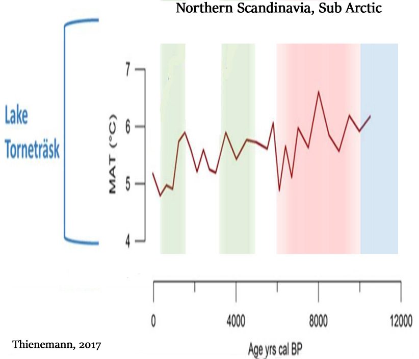
Thienemann et al., 2017 [P]roxy-inferred annual MATs[annual mean air temperatures] show the lowest value at 11,510 yr BP (7.6°C). Subsequently, temperatures rise to 10.7°C at 9540 yr BP followed by an overall decline of about 2.5°C until present (8.3°C).
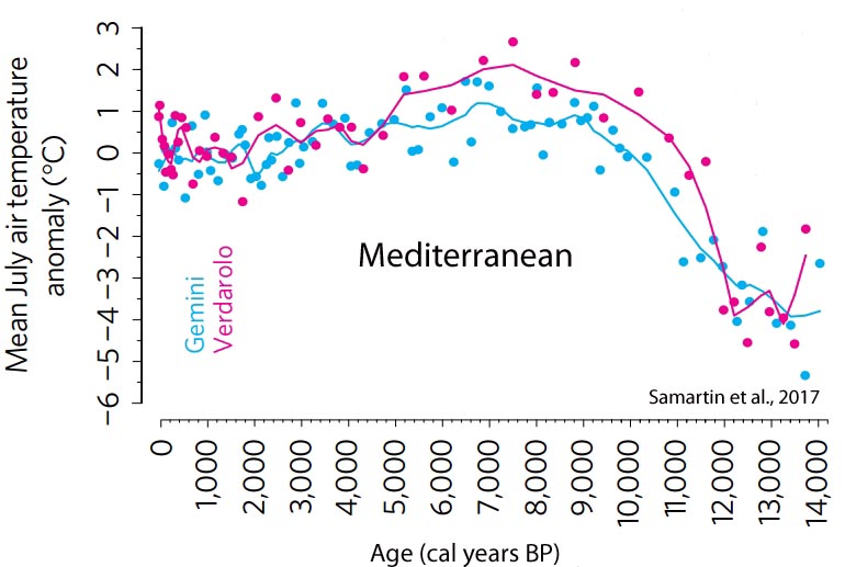
Samartin et al., 2017
Wu et al., 2017 The alkenone-based SST reconstruction shows rapid warming in the first 1500 years of the Holocene … an increase of sea surface temperature from c. 23.0 °C to 27.0 °C, associated with a strengthened summer monsoon from c. 10,350 to 8900 cal. years BP. This was also a period of rapid sea-level rise and marine transgression, during which the sea inundated the palaeo-incised channel … In these 1500 years, fluvial discharge was strong and concentrated within the channel, and the high sedimentation rate (11.8 mm/yr [1.18 m per century]) was very close to the rate of sea-level rise.

Li et al., 2017
Dodrill et al., 2017 These archaeological reconstructions of average palaeo-SST during the 1500–1100 cal BP time-period suggest that the nearshore environments of Palau were slightly warmer than those today by approximately 1–2°C.

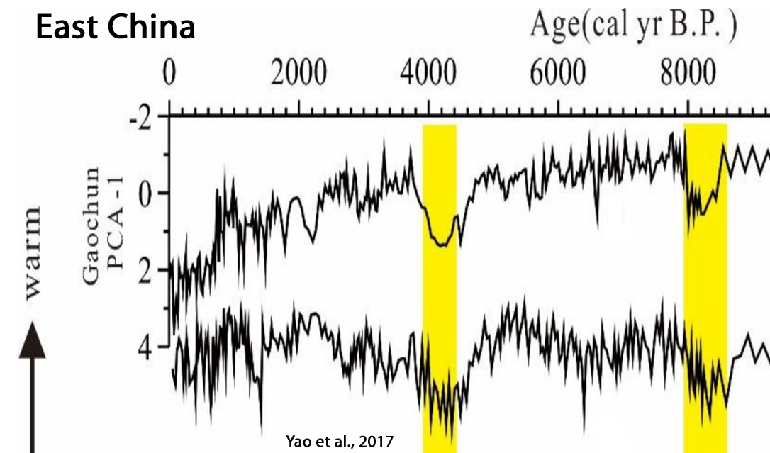
Yao et al., 2017
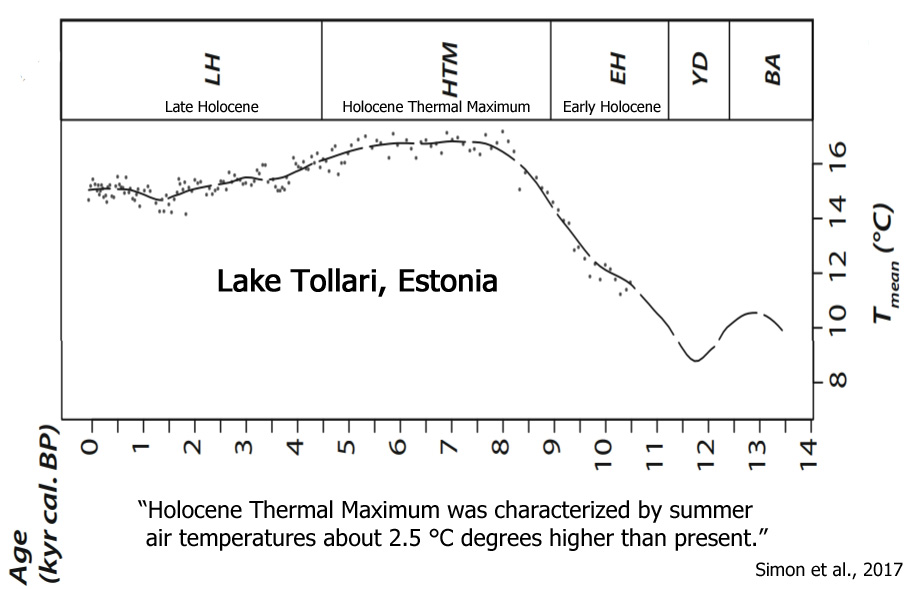
Simon et al., 2017 The Holocene coldest temperatures were observed during the Early Holocene, but temperature followed a gradual rise (from ca. 11.7 to 8 kyr cal. BP) to reach its maximal value during the Holocene Thermal Maximum (from ca. 8 to 4.5 kyr cal. BP). Holocene Thermal Maximum was characterized by summer air temperatures about 2.5 °C degrees higher than present.
Granger et al., 2017
Zhang et al., 2017

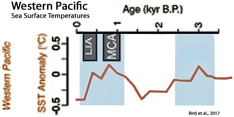
Bird et al., 2017
Reid, 2017 (Globe) The small increase in global average temperature observed over the last 166 years is the random variation of a centrally biased random walk. It is a red noise fluctuation. It is not significant, it is not a trend and it is not likely to continue.
Pendea et al., 2017 (Russia) The Holocene Thermal Maximum (HTM) was a relatively warm period that is commonly associated with the orbitally forced Holocene maximum summer insolation (e.g., Berger, 1978; Bartlein et al., 2011). Its timing varies widely from region to region but is generally detected in paleorecords between 11 and 5 cal ka BP (e.g., Kaufman et al., 2004; Bartlein et al., 2011; Renssen et al., 2012). … In Kamchatka, the timing of the HTM varies. Dirksen et al. (2013) find warmer-than-present conditions between 9000 and 5000 cal yr BP in central Kamchatka [Russia] and between 7000 and 5800 cal yr BP at coastal sites.
Stivrins et al., 2017 (Latvia) Using a multi-proxy approach, we studied the dynamics of thermokarst characteristics in western Latvia, where thermokarst occurred exceptionally late at the Holocene Thermal Maximum. … [A] thermokarst active phase … began 8500 cal. yr BP and lasted at least until 7400 cal. yr BP. Given that thermokarst arise when the mean summer air temperature gradually increased ca. 2°C beyond the modern day temperature, we can argue that before that point, the local geomorphological conditions at the study site must have been exceptional to secure ice-block from the surficial landscape transformation and environmental processes.
Bañuls-Cardona et al., 2017 During the Middle Holocene we detect important climatic events. From 7000 to 6800 [years before present] (MIR 23 and MIR22), we register climatic characteristics that could be related to the end of the African Humid Period, namely an increase in temperatures and a progressive reduction in arboreal cover as a result of a decrease in precipitation. The temperatures exceeded current levels by 1°C [Spain], especially in MIR23, where the most highly represented taxon is a thermo-Mediterranean species, M. (T.) duodecimcostatus.
Åkesson et al., 2017 (Norway) Reconstructions for southern Norway based on pollen and chironomids suggest that summer temperatures were up to 2 °C higher than present in the period between 8000 and 4000 BP, when solar insolation was higher (Nesje and Dahl, 1991; Bjune et al., 2005; Velle et al., 2005a).
Sugden et al., 2017 [T]he interior Antarctic continent had summers warm enough for tundra vegetation to grow and for mountain glaciers to consist of ice at the pressure melting point.
(press release) Central parts of Antarctica’s ice sheet have been stable for millions of years, from a time when conditions were considerably warmer than now, research suggests. By mapping and analysing surface rocks—including measuring their exposure to cosmic rays – researchers calculated that the mountains have been shaped by an ice sheet over a million-year period, beginning in a climate some 20C warmer than at present. … The last time such climates existed in the mountains of Antarctica was 14 million years ago when vegetation grew in the mountains and beetles thrived. Antarctica’s climate at the time would be similar to that of modern day Patagonia or Greenland.
Molnár and Végvári, 2017 (SE Central Europe) Our study provides an estimate for the value of MAT of HTM of Pannon region with an interval of 0.4°C, relying on macroecological considerations. We calculate the temperature of the HTM [Holocene Thermal Maximum] 1.3–1.7°C warmer than the present temperature.
Lusas et al., 2017 (East Greenland) The lack of glacio-lacustrine sediments throughout most of the record suggests that the ice cap was similar to or smaller than present throughout most of the Holocene. This restricted ice extent suggests that climate was similar to or warmer than present, in keeping with other records from Greenland that indicate a warm early and middle Holocene. Middle Holocene magnetic susceptibility oscillations, with a ~200-year frequency in one of the lakes, may relate to solar influence on local catchment processes. … Air temperatures in Milne Land, west of our study area, based on preliminary estimates from chironomids, may have been 3–6°C warmer than at present (Axford et al. 2013), and in Scoresby Sund itself, warm ocean fauna, including Mytilus edulis and Chlamys islandica, both of which live far to the south today, occupied the fjords (Sugden and John 1965; Hjort and Funder 1974; Street 1977; Funder 1978; Bennike and Wagner 2013; Fig. 13). … Recession of Istorvet ice cap in the last decade has revealed plant remains that show that the glacier was smaller than at present during the early stages of the Medieval Warm Period, but expanded during the late Holocene ca. AD 1150 (Lowell et al. 2013).
Elmslie, 2017 The Holocene Thermal Maximum (HTM) was a period of enhanced warmth during the early-to- mid Holocene period largely caused by enhanced solar insolation. In northwestern Ontario, the HTM was characterized by a lower abundance of Picea pollen and an increase in Cupressaceae and Ambrosia pollen. Pollen-based inferences suggest HTM temperatures were elevated by approximately 2-3°C [above present], and lake levels were regionally lower than today, suggesting warmer and more arid conditions than today. This warming resulted in increased algal production and associated cyanobacteria blooms in lakes in northwestern Ontario. In northeastern Ontario, climate projections suggest the HTM was 2-3°C warmer.
Abrupt, Degrees-Per-Decade Natural Global Warming (D-O Events) (7)
Sánchez et al., 2017 The estimated increases in Greenland atmospheric temperature were 5–16°C [Capron et al., 2010] and the duration of the warming events between 10 to 200 years [Steffensen et al., 2008].

Jensen et al., 2017 The Dansgaard-Oeschger (DO) events of the last glacial are some of the most prominent climate variations known from the past. Ice cores from Greenland show multiple temperature excursions during the last glacial period as the climate over Greenland alternated between cold stadial (Greenland Stadial, GS), and warmer interstadial (Greenland Interstadial, GI) conditions with a period of roughly 1500 years (Grootes and Stuiver, 1997). Each DO-event is characterised by an initial temperature rise of 10±5 °C toward GI [Greenland Interstadial] conditions in a few decades, a more gradual cooling over the following several hundreds of years, and a relatively rapid temperature drop back to GS at the end of most of the events (Johnsen et al., 1992; Dansgaard et al., 1993; North-Greenland-Ice-Core-project members, 2004; Kindler et al., 2014). DO-events are manifested not only in Greenland, but around the world
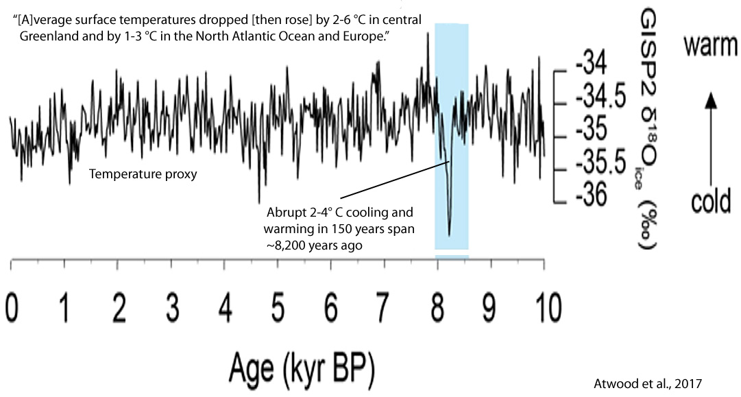
Atwood et al., 2017 The relatively stable climate of the Holocene epoch (11,700 yr BP-present) was punctuated by a period of large and abrupt climate change ca. 8,200 yr BP, when an outburst of glacial meltwater into the Labrador Sea drove large and abrupt climate changes across the globe. Polar ice and marine records indicate that annual average surface temperatures dropped by 2-6 °C in central Greenland and by 1-3 °C in the North Atlantic Ocean and Europe [within decades]. The associated climate perturbations are generally thought to have persisted for 100-150 years [before temperatures returned to the previous baseline]. … These events stretch our understanding of the dynamical principles that govern the climate system, given the lack of these events in the modern record and the inability of climate models to reproduce such variability.
Lynch-Stieglitz, 2017 Abrupt changes in climate have occurred in many locations around the globe over the last glacial cycle, with pronounced temperature swings on timescales of decades or less in the North Atlantic. The global pattern of these changes suggests that they reflect variability in the Atlantic meridional overturning circulation (AMOC). … In many locations in the Northern Hemisphere, abrupt changes in climate have occurred that span almost the full range of glacial to interglacial conditions, with the transition between climate states occurring in decades or less (Alley & Clark 1999, Voelker 2002). These abrupt climate changes are most clearly recorded in the climate records from glacial ice on Greenland (Andersen et al. 2004) and are referred to as DansgaardOeschger (D-O) events. The warm intervals are referred to as interstadials, and the cold intervals are referred to as stadials. … [T]he prevailing paradigm is that the abrupt climate changes are a result of changes in the northward transport of heat by the Atlantic meridional overturning circulation (AMOC) (Broecker et al. 1985, Clark et al. 2002, Rahmstorf 2002).
Ivanovic et al., 2017 During the Last Glacial Maximum 26–19 thousand years ago (ka), a vast ice sheet stretched over North America [Clark et al., 2009]. In subsequent millennia, as climate warmed and this ice sheet decayed, large volumes of meltwater flooded to the oceans [Tarasov and Peltier, 2006; Wickert, 2016]. This period, known as the “last deglaciation,” included episodes of abrupt climate change, such as the Bølling warming [~14.7–14.5 ka], when Northern Hemisphere temperatures increased by 4–5°C in just a few decades [Lea et al., 2003; Buizert et al., 2014], coinciding with a 12–22 m sea level rise in less than 340 years [5.3 meters per century] (Meltwater Pulse 1a (MWP1a)) [Deschamps et al., 2012].

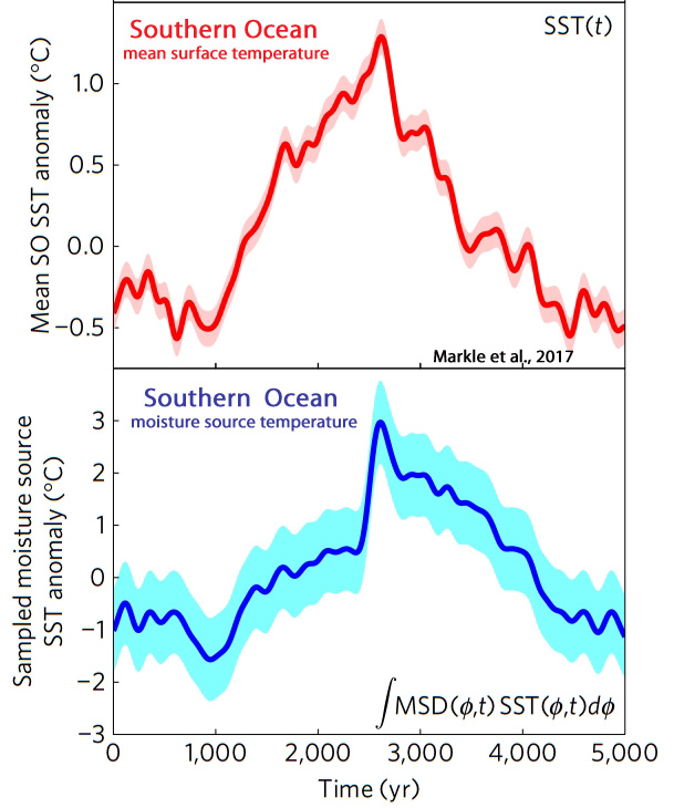
Markle et al., 2017 The temperature relationship between the hemispheres is commonly attributed to an interhemispheric redistribution of heat by the ocean overturning circulation. Changes in ocean heat transport should be accompanied by changes in atmospheric circulation to satisfy global energy budget constraints. Although changes in tropical atmospheric circulation linked to abrupt events in the Northern Hemisphere are well documented, evidence for predicted changes in the Southern Hemisphere’s atmospheric circulation during Dansgaard–Oeschger cycles is lacking. Here we use a high-resolution deuterium-excess record from West Antarctica to show that the latitude of the mean moisture source for Antarctic precipitation changed in phase with abrupt shifts in Northern Hemisphere climate, and significantly before Antarctic temperature change. This provides direct evidence that Southern Hemisphere mid-latitude storm tracks shifted within decades of abrupt changes in the North Atlantic, in parallel with meridional migrations of the intertropical convergence zone. We conclude that both oceanic and atmospheric processes, operating on different timescales, link the hemispheres during abrupt climate change.
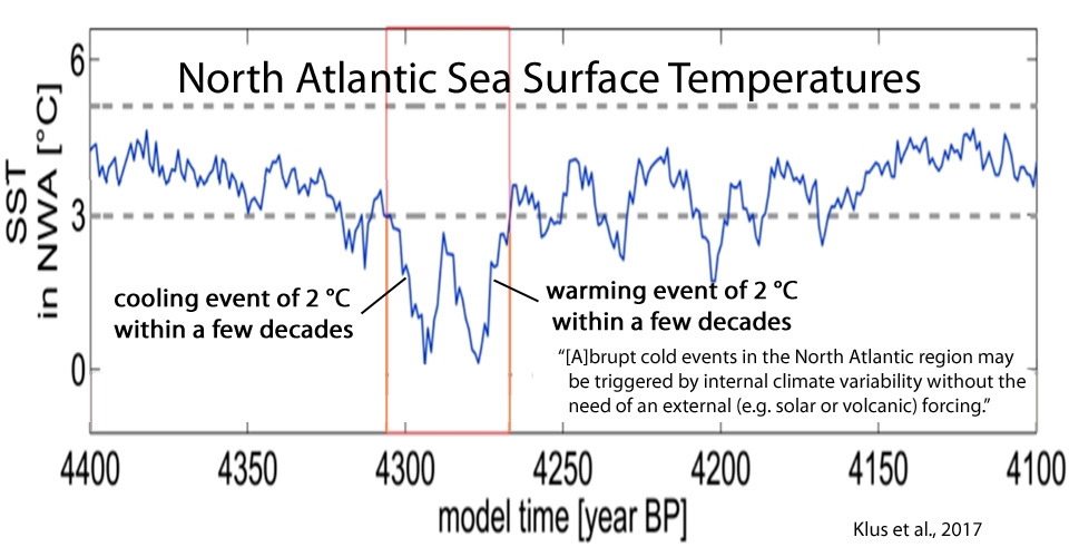
Klus et al., 2017 Abrupt cold events have been detected in numerous North Atlantic climate records from the Holocene. … Here, we describe two cold events that occurred during an orbitally forced transient Holocene simulation using the Community Climate System Model version 3. Both events occurred during the late Holocene (event 1 referring to 4305-4267 BP [38 years] and event 2 referring to 3046-3018 BP [28 years]) and were characterized by substantial surface cooling (-2.7 and -2.2 °C, respectively [-0.71 °C/per decade and -0.78 °C/decade]) … … Northeast of Iceland, however, shows an increase in both SST and SSS, but a decline in sea ice concentration (event 1: warming of 1.6 °C [+0.42 °C/decade], rise of 0.7 PSU, decline of -5 % in sea ice concentration; event 2: warming of 1.9 °C [+0.68 °C/decade], rise of 0.9 PSU, decline of -11 % in sea ice concentration). … The events were triggered by prolonged phases of a positive North Atlantic Oscillation which, through changes in surface winds, caused substantial changes in the sub-polar ocean circulation and associated freshwater transports, resulting in a weakening of the sub-polar gyre. Our results suggest a possible mechanism by which abrupt cold events in the North Atlantic region may be triggered by internal climate variability without the need of an external (e.g. solar or volcanic) forcing.
A Model-Defying Cryosphere, Polar Ice (33)
Årthun et al., 2017 Statistical regression models show that a significant part of northern climate variability thus can be skillfully predicted up to a decade in advance based on the state of the ocean. Particularly, we predict that Norwegian air temperature will decrease over the coming years, although staying above the long-term (1981–2010) average. Winter Arctic sea ice extent will remain low but with a general increase towards 2020.
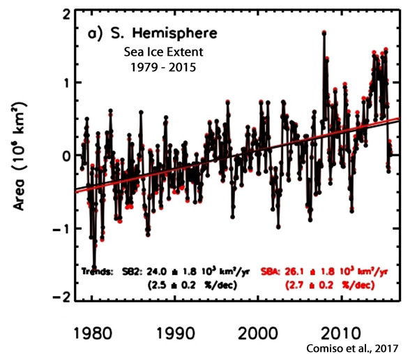
Comiso et al., 2017 The Antarctic sea ice extent has been slowly increasing contrary to expected trends due to global warming and results from coupled climate models. After a record high extent in 2012 the extent was even higher in 2014 when the magnitude exceeded 20 × 106 km2 for the first time during the satellite era. … [T]he trend in sea ice cover is strongly influenced by the trend in surface temperature [cooling]. … A case study comparing the record high in 2014 with a relatively low ice extent in 2015 also shows strong sensitivity to changes in surface temperature. The results suggest that the positive trend is a consequence of the spatial variability of global trends in surface temperature and that the ability of current climate models to forecast sea ice trend can be improved through better performance in reproducing observed surface temperatures in the Antarctic region.
Baggett and Lee, 2017 The dynamical mechanisms that lead to wintertime Arctic warming during the planetary-scale wave (PSW) and synoptic-scale wave (SSW) life cycles are identified by performing a composite analysis of ERA-Interim reanalysis data. The PSW life cycle is preceded by localized tropical convection over the Western Pacific. Upon reaching the mid-latitudes, the PSWs amplify as they undergo baroclinic conversion and constructively interfere with the climatological stationary waves. The PSWs [natural planetary scale waves] flux large quantities of sensible and latent heat into the Arctic which produces a regionally enhanced greenhouse effect that increases downward IR and warms the Arctic two-meter temperature. The SSW life cycle is also capable of increasing downward IR and warming the Arctic two-meter temperature, but the greatest warming is accomplished in the subset of SSW events with the most amplified PSWs. Consequently, during both the PSW and SSW life cycles, wintertime Arctic warming arises from the amplification of the PSWs [natural planetary scale waves].
Brun et al., 2017 We provide spatially resolved estimates for the potential contribution of HMA [High Mountain Asia] glaciers to SLR [sea level rise] and changes in the downstream hydrology, aggregated by major river basins. We find a total sea level contribution of -16.3 ± 3.5 Gt yr−1 (14.6 ± 3.1 Gt yr−1 when including only the exorheic basins), corresponding to 0.046 ± 0.009 mm yr−1 sea level equivalent (SLE) (0.041 ± 0.009 mm yr−1 SLE when including only the exorheic basins). … This estimate is in marked disagreement with the total estimate of −46 ± 15 Gt yr−1 from Cogley, 2009 and Marzeion et al., 2015 commonly used in the sea level budget studies. … The model contribution estimates of Cogley, 2009 and Marzeion et al., 2015 for the period 2000–2013 are nearly four times larger than our estimate for Central Asia (22 Gt yr−1 for the model versus 6 Gt yr−1 for this study) and over twice as large for South Asia East and South Asia West (14 Gt yr−1 for the model versus 6 Gt yr−1 for this study, and 9 Gt yr−1 for the model versus 4 Gt yr−1 for this study for the two regions respectively. …These discrepancies can be explained by the lack of direct measurements to constrain both the interpolation method of Cogley, 2009 and the model tuning and/or the high temporal smoothness of atmospheric models of Marzeion et al., 2015. In particular, these estimates [Cogley, 2009 and Marzeion et al., 2015] attribute mass losses to Karakoram and Kunlun, two regions with a large glacierized area where we find only little mass loss or even mass gain. … Our new estimate of HMA [High Mountain Asia] glacier contribution to SLR [sea level rise] for 2000–2016 (0.041 ± 0.009 mm yr−1 SLE [sea level equivalent], when excluding endorheic basins) is slightly smaller than the values of Kääb et al., 2015 (0.06 ± 0.01 mm yr−1 SLE) and Gardner et al., 2013 (0.07 ± 0.03 mm yr−1 SLE), but much smaller than the model-based estimate of Cogley, 2009 and Marzeion et al., 2015 (0.13 ± 0.05 mm yr−1 SLE), although the latter are widely used in the literature.
Chand et al., 2017 Introduction: The LIA [Little Ice Age] is a globally documented cooling event that began around the 13th or 14th century and culminated between the mid- 16th and mid-19th centuries. Although the cause of LIA glaciation is not fully understood, climatologists contend that reduced solar output, changes in atmospheric circulation as a result of a reversal of the North Atlantic Oscillation and explosive volcanism could have decreased the global temperature. … Based on the GSI’s repeated photographs of 1906, 1956 and 1963, and the position of the recessional moraine ridges, it is clear that the lower frontal tongue of the Bara Shigri Glacier changed significantly from 1906 to 1965 (59 years). During this period, a loss 1.8 +/- 0.52 km2 in glacier area occurred at an annual rate of 0.03 +/- 0.02 km2 … The total frontal area vacated by the glacier for the period between 1965 and 2014 is 1.1 +/- 0.01 km2 with an annual rate of 0.02 +/- 0.0003 km2. [Glacier recession was 1.8 km2 and -0.03 km2 per year for 1906-1965 (59 years), with a 30-40% deceleration to 1.1 km2 and -0.02 km2 per year for 1965-2014 (59 years)]
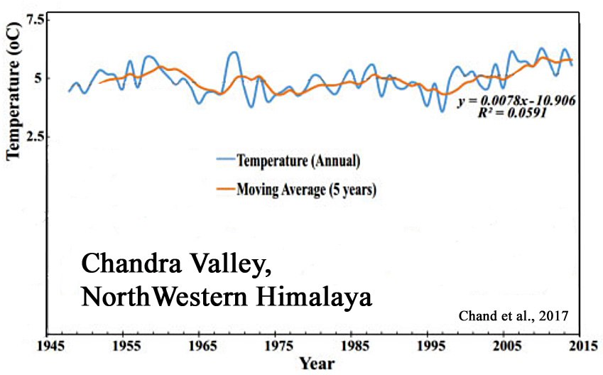
Forsythe et al., 2017 Karakoram temperature and glacial melt driven by regional atmospheric circulation variability … Streamflows dependent on glacial meltwater are strongly positively correlated with Karakoram summer air temperatures, which show recent anomalous cooling.
Bader et al., 2017 Rather than reflecting major changes in ice flow path over time, the provenance changes are interpreted to indicate relative stability of the East Antarctic ice sheet
Leeson et al, 2017 Melt water from the Greenland ice sheet contributed 1.7–6.12 mm [0.39 of a centimeter median] to global sea level between 1993 and 2010 [0.39 cm in 17 years = 0.23 mm/yr-1]
Van der Bilt et al., 2017 Late Holocene glacier reconstruction reveals retreat behind present limits … Regional palaeoclimate evidence from the adjoining Southern Ocean region also reveal contemporaneous shifts. For example, reconstructed sea surface temperatures (SSTs) west of the Antarctic Peninsular rose 3 ˚C in less than a century (Shevenell et al., 2011). … Following the termination of a Late Holocene glacier maximum around 1250 cal a BP, warming created conditions unfavourable for glacier growth during the regional expression of an MCA [Medieval Climate Anomaly] between 950 and 700 cal a BP (Villalba, 1994). From 500 cal a BP, the Hamberg overspill glacier rapidly retreated behind its present-day position, possibly driven by local warming and/or major shifts in regional atmospheric and oceanic circulation patterns (Moy et al., 2008; Shevenell et al., 2011; Abram et al., 2014; Foster et al., 2016).
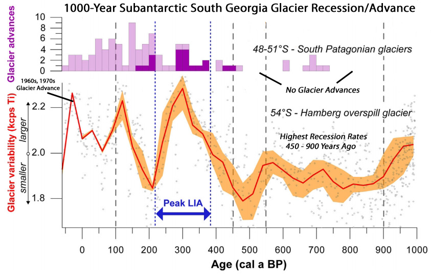
Orsi et al., 2017 The recent warming trend in North Greenland … We find that δ 18O [temperature/climate proxy] has been increasing over the past 30 years, and that the decade 1996-2005 is the second highest decade in the 287-year record. The highest δ 18O [temperature/climate proxy] values were found in 1928, which is also an extreme year in GISP2 and NGRIP ice cores, and in a coastal South Greenland composite (Vinther et al., 2006; Masson-Delmotte et al., 2015), but the decadal average (1926-1935) is not statistically different from the decade (2002-2011). … The surface warming trend has been principally attributed to sea ice retreat and associated heat fluxes from the ocean (Serreze et al., 2009; Screen and Simmonds, 2010a, b), to a negative trend in the North Atlantic Oscillation (NAO) since 1990, increasing warm air advection on the West Coast of Greenland and Eastern Canada (Hanna et al., 2012; Fettweis et al., 2013; Ding et al., 2014), and to an increase in the Greenland Blocking Index [Hanna et al., 2013]. These latter mechanisms could be dominated by natural variability rather than forced response to the anthropogenic increase in greenhouse gases (Fettweis et al., 2013; Screen et al., 2014).
Brinkerhoff et al., 2017 Most of Earth’s glaciers are retreating, but some tidewater glaciers are advancing despite increasing temperatures and contrary to their neighbors. This can be explained by the coupling of ice and sediment dynamics: a shoal forms at the glacier terminus, reducing ice discharge and causing advance towards an unstable configuration followed by abrupt retreat, in a process known as the tidewater glacier cycle. Here we use a numerical model calibrated with observations to show that interactions between ice flow, glacial erosion, and sediment transport drive these cycles, which occur independent of climate variations. Water availability controls cycle period and amplitude, and enhanced melt from future warming could trigger advance even in glaciers that are steady or retreating, complicating interpretations of glacier response to climate change. The resulting shifts in sediment and meltwater delivery from changes in glacier configuration may impact interpretations of marine sediments, fjord geochemistry, and marine ecosystems.
Spector et al., 2017 Rapid Thinning of Southern Ross Sea Glaciers – Scott Glacier Below the summit of Mt Rigby, exposure ages decrease with elevation and record rapid thinning of Scott Glacier at ∼8.4 and ∼6.3 kyr BP. After the second of these events, the ice surface gradually lowered over the next ∼3 kyr to near the modern glacier level. … Beardmore Glacier Erratics from Mt Hope’s southeast ridge record gradual thinning of the margin of Beardmore Glacier to an elevation of 440 m by ∼9.3 kyr BP. The ice surface then abruptly dropped ∼280 m over the next 700 ± 200 years to within 80 m of the modern glacier level. … Geologic data from around the continent show deglaciation continuing into the late Holocene, long after MWP-1A [meltwater pulse, 14,600 years ago]. None of this evidence is consistent with an Antarctic source for the enormous volume of meltwater released to the oceans in a few hundred years during MWP-1A.
Doddridge and Marshall, 2017 Through analysis of remotely-sensed sea surface temperature (SST) and sea ice concentration data we investigate the impact of winds related to the Southern Annular Mode (SAM) on sea ice extent around Antarctica. We show that positive SAM anomalies in the austral summer are associated with anomalously cold SSTs that persist and lead to anomalous ice growth in the following autumn, while negative SAM anomalies precede warm SSTs and a reduction in sea ice extent during autumn. … Our analysis shows that the wind anomalies related to the negative SAM during the 2016/17 austral summer contributed to the record minimum Antarctic sea ice extent observed in March 2017.
Cerrone and Fusco, 2017 Compelling evidence indicates that the large increase in the SH [Southern Hemisphere] sea ice, recorded over recent years, arises from the impact of climate modes and their long–term trends. The examination of variability ranging from seasonal to interdecadal scales, and of trends within the climate patterns and total Antarctic sea ice concentration (SIC) for the 32–yr period (1982–2013) are the key focuses of this paper. Our results indicate that a progressive cooling affected the year–to–year climate of the sub–Antarctic since 1990s. This feature is found in association with increased positive SAM and SAO phases detected in terms of upward annual and seasonal trends (in autumn and summer), and upward decadal trends. In addition, the SIC shows upward annual, spring and summer trends, indicating the insulation of Antarctica from the warmer flows in the midlatitudes.
Mezgec et al., 2017 The causes of the recent increase in Antarctic sea ice extent, characterised by large regional contrasts and decadal variations, remain unclear. … Simulations performed with state-of-the-art climate models fail to capture such a sea ice increase. The mechanisms that drive Antarctic sea ice changes, and the respective roles of internal climate variability vs. natural and anthropogenic forcing remain debatable. … Altogether, these results point out that katabatic winds are the major players in pack ice formation and thickening of landfast ice, while geostrophic winds are driving the export and extension of pack ice in WRS. This calls for the development of coupled ocean-atmosphere models that can incorporate the interplay between katabatic/geostrophic winds and sea ice formation in latent-heat polynyas and their export to the open ocean.
Ding et al., 2017 The Arctic has seen rapid sea-ice decline in the past three decades, whilst warming at about twice the global average rate. … Internal variability dominates the Arctic summer circulation trend and may be responsible for about 30–50% of the overall decline in September sea ice since 1979.
(press release) [A] substantial chunk of summer sea ice loss in recent decades was due to natural variability in the atmosphere over the Arctic Ocean.
Fernandoy et al., 2017 The firn stable isotope composition reveals that the near–surface temperature at the Antarctic Peninsula shows a decreasing trend (−0.33 °C y−1) between 2008 and 2014.
Thomas et al., 2017 Our results show that SMB [surface mass balance] for the total Antarctic Ice Sheet (including ice shelves) has increased at a rate of 7 ± 0.13 Gt decade−1 since 1800 AD representing a net reduction in sea level of ∼ 0.02 mm decade−1 since 1800 and ∼ 0.04 mm decade−1 since 1900 AD. The largest contribution is from the Antarctic Peninsula (∼ 75 %) where the annual average SMB during the most recent decade (2001–2010) is 123 ± 44 Gt yr−1 higher than the annual average during the first decade of the 19th century.
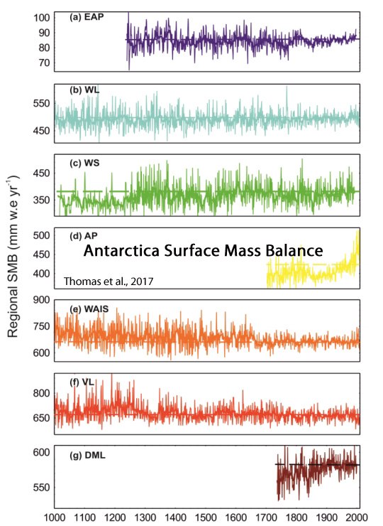
Goel et al., 2017 Ice rises are a useful resource to investigate evolution and past climate of the DML coastal region. We investigate Blåskimen Island ice rise, one of the larger isle-type ice rises at the calving front of the intersection of Fimbul and Jelbart Ice Shelves, using geophysical methods. … Using the Input-Output method for a range of parameters and column setups, we conclude that Blåskimen Island has been thickening over the past nine years [2005-2014]. Thickening rates cannot be determined precisely, but ensemble results show that thickening rate averaged over the ice rise varies between 0.07 m a−1 and 0.35 m a−1 [per year]. On longer timescales, we speculate that the summit of Blåskimen Island has been stable within several kilometers at least in the past ∼600 years but no longer than several millennia.
Kim et al., 2017 Understanding the Mechanism of Arctic Amplification and Sea Ice Loss … Sea ice reduction is accelerating in the Barents and Kara Seas. Several mechanisms are proposed to explain the accelerated loss of polar sea ice, which remains an open question. [CO2 is not mentioned anywhere in the paper as a mechanism responsible for Arctic amplification or sea ice loss.]
Oliva et al., 2017 However, a recent analysis (Turner et al., 2016) has shown that the regionally stacked temperature record for the last three decades has shifted from a warming trend of 0.32 °C/decade during 1979–1997 to a cooling trend of − 0.47 °C/decade during 1999–2014. … This recent cooling has already impacted the cryosphere in the northern AP [Antarctic Peninsula], including slow-down of glacier recession, a shift to surface mass gains of the peripheral glacier and a thinning of the active layer of permafrost in northern AP islands.
Martín-Español et al., 2017 We investigate the mass balance of East Antarctica for 2003–2013 using a Bayesian statistical framework. … We apportion mass trends to SMB and ice dynamics for the EAIS, based on two different assumptions, different remote sensing data and two RCMs. In the first experiment, the model apportions about a third of the mass trend to ice dynamics, +17 Gt/yr, and two thirds, +40 Gt yr−1 to SMB, resulting in a total mass trend for the EAIS [East Antarctic Ice Sheet] of +57 ± 20 Gt yr−1.
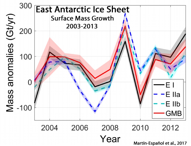
Pittard et al., 2017 We suggest the Lambert-Amery glacial system will remain stable, or gain ice mass and mitigate a portion of potential future sea level rise over the next 500 years, with a range of +3.6 to -117.5 mm GMSL-equivalent.
Fettweis et al ., 2017 Results from all MAR simulations indicate that (i) the period 1961–1990, commonly chosen as a stable reference period for Greenland SMB and ice dynamics, is actually a period of anomalously positive SMB (∼ +40 Gt yr−1 ) compared to 1900–2010 … [T]he ERA-20C forced simulation suggests that SMB [surface mass balance] during the 1920–1930 warm period over Greenland was comparable to the SMB of the 2000s, due to both higher melt and lower precipitation than normal. … The period 1961–1990 has been considered as a period when the total mass balance of the Greenland ice sheet was stable (Rignot and Kanagaratnam, 2006) and near zero. However, at the last century scale, all MAR reconstructions suggest that SMB [surface mass balance] was particularly positive during this period [1961-1990] (SMB was most positive from the 1970s to the middle of the 1990s), suggesting that mass gain may well have occurred during this period, in agreement with results from Colgan et al. (2015). Finally, with respect to the 1961–1990 period, the integrated contribution of the GrIS SMB anomalies over 1900–2010 is a sea level rise of about 15 ± 5 mm [1.35 cm per century], with a null contribution from the 1940s to the 2000s, suggesting that the recent contribution of GrIS to sea level change (van den Broeke et al., 2016) is unprecedented in the last century.
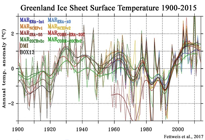
Reeves Eyre and Zeng, 2017 Ice sheet-average annual mean SAT [surface air temperatures] from different datasets are highly correlated in recent decades, but their 1901–2000 trends differ even in sign [Greenland cooled]. Compared with the MERRA2 climatology combined with gridded SAT analysis anomalies, thirty-one earth system model historical runs from the CMIP5 archive [biases] reach ~5°C for the 1901–2000 average bias and have opposite trends [modeled warming when Greenland was cooling] for a number of sub-periods. … Due to its remoteness and extreme climate however, continuous widespread climate monitoring over the GrIS has been carried out for only about the last two decades, and even then with rather sparse coverage in some geographic areas and glaciological regimes. … Box (2002) found a pattern of warming from ~1900 to ~1940, cooling from ~1940 to ~1990, and warming from ~1990 onwards. In addition, inter-annual variability was found to be closely related to the North Atlantic Oscillation (NAO). …Biases vary by season and by region of the ice sheet: in the ablation region (demarcated here by the 1500 m elevation contour) during summer, most reanalyses have a ~1°C positive bias (though 20CR and ERA–20C have negative biases) while CRU and Berkeley Earth gridded SAT analyses have larger positive biases.
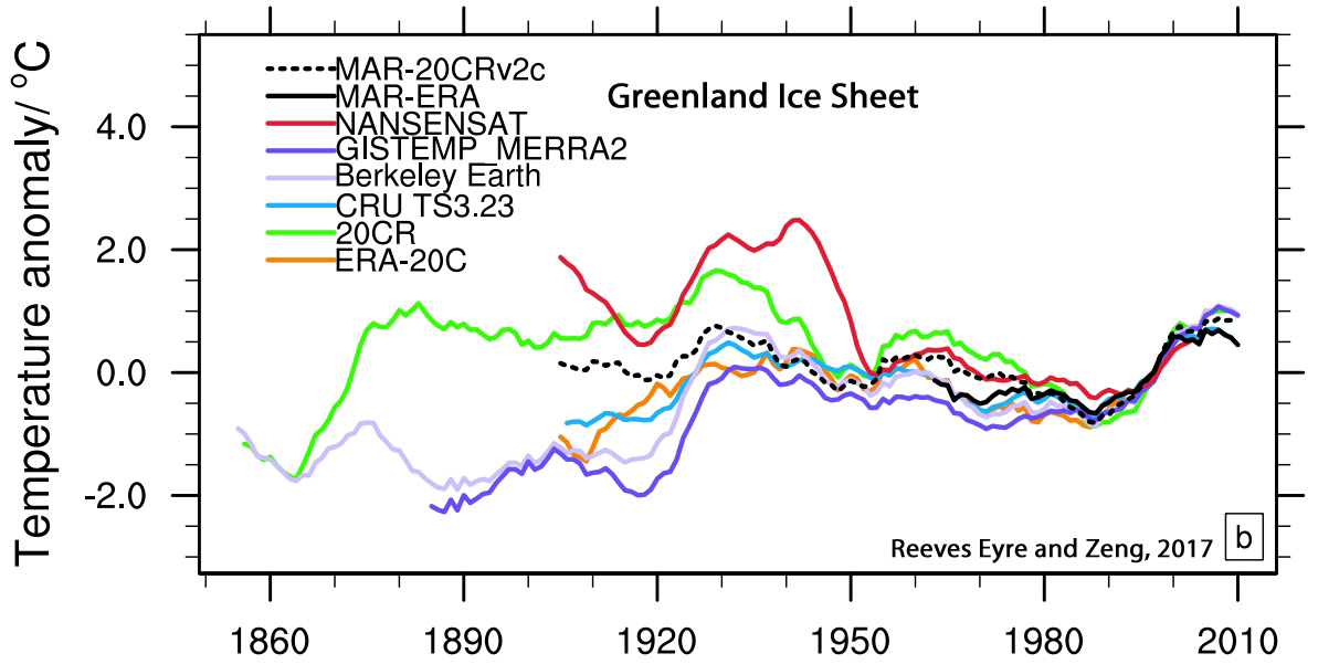
van der Bilt et al., 2017 [R]econstruction of glacier variations over the past ∼1250 years. Together with local moraine evidence and supporting evidence from other Southern Hemisphere glaciers on New Zealand and in Patagonia, our findings reveal a series of consecutively diminishing Late Holocene advances. In addition to a glacier maximum before 1250 cal a BP, these include a two-stage Little Ice Age with advances around 300 and 120 cal a BP, in line with evidence from southern Patagonia. In addition, we present evidence for an unreported [glacier] retreat behind present limits around 500 cal BP.
Fogt et al., 2017 At their peak on 6 December 1911, the temperatures measured by Amundsen exceeded -16°C, which represents an anomaly relative to our estimate from ERA-Int climatology [long-term temperature and pressure record] of more than 10°C. … Amundsen’s sledging temperature measurements during this time are much warmer than the hourly and daily mean observations collected at the South Pole station since 1957, even when accounting for the average differences in temperature between Amundsen’s location and the South Pole, which is often colder than nearby areas due to pooling of cold air in the slightly lower elevation (Comiso 2000). The daily mean temperature measured at the South Pole on December 7, 2015 of -19.8°C (max hourly temperature of -18.2°C) is the only comparable warm day before December 11th, otherwise observed South Pole daily mean temperatures have never exceeded -20°C in this portion of early summer [since 1911]. … [D]aily maximum temperatures above -20°C occurred for two consecutive days in 2015 and 2012, but these are quite warm exceptions to the normal conditions (Fig. S9). In contrast, Amundsen experienced four continuous days with daily mean temperatures exceeding -19.0°C and temperature anomalies from the ERA-Int climatology greater than 10°C. … Notably, there is a large positive spike during summer 1911/12, when seasonal mean pressures rise above 1000 hPa. The reconstruction pre-1957 shows only one other summer with pressures above 1000 hPa, in 1925/26, as discussed in Fogt et al. (2016b), while the direct observations display one summer in 1976/77 when they exceed 1000 hPa. This ranks the McMurdo pressure during the summer of the South Pole races [summer 1911/12] in the top three highest over the last 110 years. … Scott’s absolute difference of 19.58°C and anomaly difference of 12.58°C clearly stand out as unique: in only one year during 1979-2015 was there a similar large swing in temperatures on these days.
Schroeter et al., 2017 Antarctic sea ice extent has increased by approximately 1.5 % per decade since satellite observations began in 1979 (Parkinson and Cavalieri, 2012; Turner et al., 2015). The small overall increase masks higher-magnitude regional and seasonal trends around the continent, most notably an increase of 3.9 % per decade in the Ross Sea peaking during spring, and a decrease of −3.4 % per decade in the Amundsen and Bellingshausen seas peaking during autumn (Turner et al., 2015). By contrast, models in the Coupled Model Intercomparison Project Phase 5 (CMIP5) exhibit decreasing sea ice trends in all months (Turner et al., 2013a). The reasons for the disparity between observed and modelled trends are not yet well understood (Bindoff et al., 2013; Hobbs et al., 2016).
Bolch et al., 2017 Previous geodetic estimates of mass changes in the Karakoram revealed balanced budgets or a possible slight mass gain since ∼ 2000. Indications of longer-term stability exist but only very few mass budget analyses are available before 2000. Here, based on 1973 Hexagon KH-9, ∼ 2009 ASTER and the SRTM DTM, we show that glaciers in the Hunza River basin (central Karakoram) were on average in balance or showed slight insignificant mass loss within the period ∼ 1973–2009.
Gagné et al., 2017 Updated observational datasets without climatological infilling show that there was an increase in sea ice concentration in the Eastern Arctic between 1950 and 1975, contrary to earlier climatology in-filled observational datasets that show weak inter-annual variations during that time period.

Connolly et al., 2017 According to this new dataset, the recent period of Arctic sea ice retreat since the 1970s followed a period of sea ice growth after the mid 1940s, which in turn followed a period of sea ice retreat after the 1910s. Our reconstructions agree with previous studies that have noted a general decrease in Arctic sea ice extent (for all four seasons) since the start of the satellite era (1979). However, the timing of the start of the satellite era is unfortunate in that it coincided with the end of several decades during which Arctic sea ice extent was generally increasing. This late-1970s reversal in sea ice trends was not captured by the hindcasts of the recent CMIP5 climate models used for the latest IPCC reports, which suggests that current climate models are still quite poor at modelling past sea ice trends. Nor is it described in previous Arctic sea ice reconstructions such as the Walsh dataset or the widely used HadISST sea ice dataset, although some recent studies have noted similar reversals, e.g. Pirón and Pasalodos (2016) and Alekseev et al. (2016).
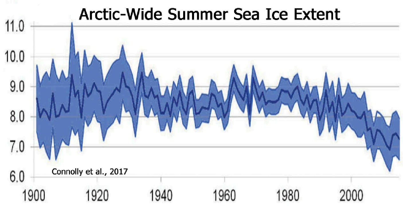

Wang et al. 2017 No evidence of widespread decline of snow cover on the Tibetan Plateau over 2000–2015 … Our results show no widespread decline in snow cover over the past fifteen years and the trends of snow cover phenology over the TP has high spatial heterogeneity.
Moffa-Sánchez and Hall, 2017 Paleoceanographic reconstructions from a more northward location of the polar front on the North Iceland margin show centennial-scale cold events and marked increases in sea ice with similar timing to the cold events recorded in the eastern Labrador Sea. … The records from the northernmost sites show a linear cooling trend perhaps driven by the Neoglacial decrease in summer insolation in the northern high latitudes and its effects on Arctic sea ice production. Periods of increased influence of polar waters in the eastern Labrador Sea, reduced LSW [Labrador Sea Water] formation and weaker subpolar gyre largely coincide with well-established cold periods recorded in glacier advances, tree-ring and pollen records in the circum-North Atlantic and northwest Europe [Dark Ages Cold Period, Little Ice Age]. Conversely, periods of reduced influence of polar waters in the eastern Labrador Sea, stronger subpolar gyre and increase LSW [Labrador Sea Water] formation largely coincide with mild/warm periods in Europe namely the Roman Warm Period and the Medieval Climatic Anomaly. These intervals are recorded as periods of glacier retreats and/or periods of no glacier advances, with milder temperatures allowing the northward expansion of vineyard crops to the North of Italy and even the British Isles. This strong correspondence in the timing of ocean and continental climate variability suggests that the ocean conditions, particularly the formation of LSW, related changes in the subpolar gyre strength, and attendant northward heat transport, were probably key in modulating the climate in northwest Europe. … [A] recent model comparison study has highlighted the inability of most climate models to correctly represent the surface mixed layer depth in the subpolar gyre region and hence likely underestimating the potential for a future collapse of the LSW formation/subpolar gyre under enhanced freshwater forcing. It is therefore essential that we continue to improve our understanding of the LSW/subpolar gyre dynamics at a range of time scales to reduce uncertainty in future climate predictions.
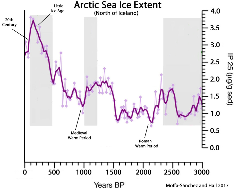
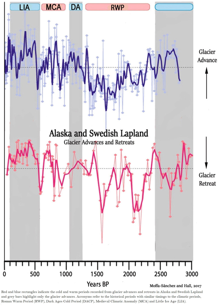
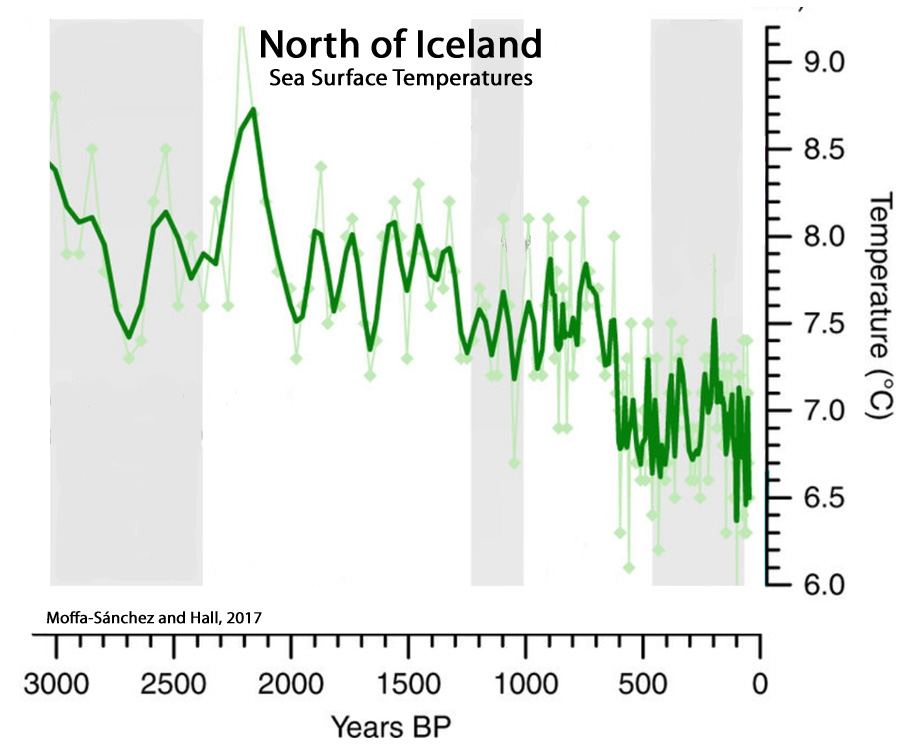
Moffa-Sánchez and Hall, 2017 (supplemental)
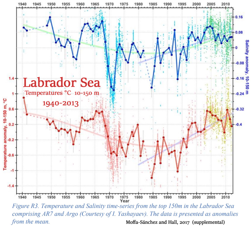
Yan et al., 2017 Afforded by continuous satellite imagery, evolution of sea ice cover over nearly three decades from 1988 to 2015 in the Bohai Sea [North China] as a peculiar mid-latitude frozen sea area is reported for the first time. An anomalous trend of slight overall increase of 1.38 ± 1.00% yr–1 (R = 1.38, i.e. at a statistical significance of 80%) in Bohai Sea ice extent was observed over the 28 year period. The detrended annual average ice area (AAIA) was further found to correlate with a slight decreasing mean ice-period average temperature of 11 meteorological stations around the Bohai Sea as well as a mild increasing cumulative freezing degree days. Correlation with decreasing Arctic Oscillation (AO) index (r = –0.60, p < 0.01) and North Atlantic Oscillation (NAO) index (r = –0.69, p < 0.01) over the study period suggested AO and NAO as the primary large-scale climate factors for Bohai Sea ice.
Hofer et al., 2017 Decreasing cloud cover drives the recent mass loss on the Greenland Ice Sheet … The Greenland Ice Sheet (GrIS) has been losing mass at an accelerating rate since the mid-1990s. … We show, using satellite data and climate model output, that the abrupt reduction in surface mass balance since about 1995 can be attributed largely to a coincident trend of decreasing summer cloud cover enhancing the melt-albedo feedback. Satellite observations show that, from 1995 to 2009, summer cloud cover decreased by 0.9 ± 0.3% per year. Model output indicates that the GrIS summer melt increases by 27 ± 13 gigatons (Gt) per percent reduction in summer cloud cover, principally because of the impact of increased shortwave radiation over the low albedo ablation zone. The observed reduction in cloud cover is strongly correlated with a state shift in the North Atlantic Oscillation promoting anticyclonic conditions in summer and suggests that the enhanced surface mass loss from the GrIS is driven by synoptic-scale changes in Arctic-wide atmospheric circulation. … Th[e] strong correlation between summertime NAO index and the MAR-based cloud cover could be used to forecast whether the observed reduction in cloud cover during summer, and the associated increase in GrIS melt, is likely to continue.
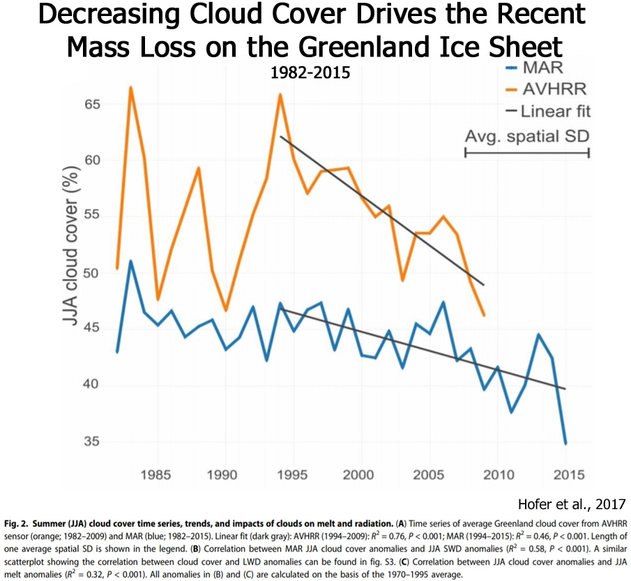
Antarctica Ice Melting In High Geothermal Heat Flux Areas (4)
Seroussi et al., 2017 Mantle plumes may more than double the geothermal heat flux above nominal continental values. … The experiments show that mantle plumes have an important local impact on the ice sheet, with basal melting rates reaching several centimeters per year directly above the hotspot.
Martos et al., 2017 Antarctica is the largest reservoir of ice on Earth. Understanding its ice sheet dynamics is crucial to unraveling past global climate change and making robust climatic and sea level predictions. Of the basic parameters that shape and control ice flow, the most poorly known is geothermal heat flux. Direct observations of heat flux are difficult to obtain in Antarctica, and until now continent-wide heat flux maps have only been derived from low-resolution satellite magnetic and seismological data. We present a high resolution heat flux map and associated uncertainty derived from spectral analysis of the most advanced continental compilation of airborne magnetic data.
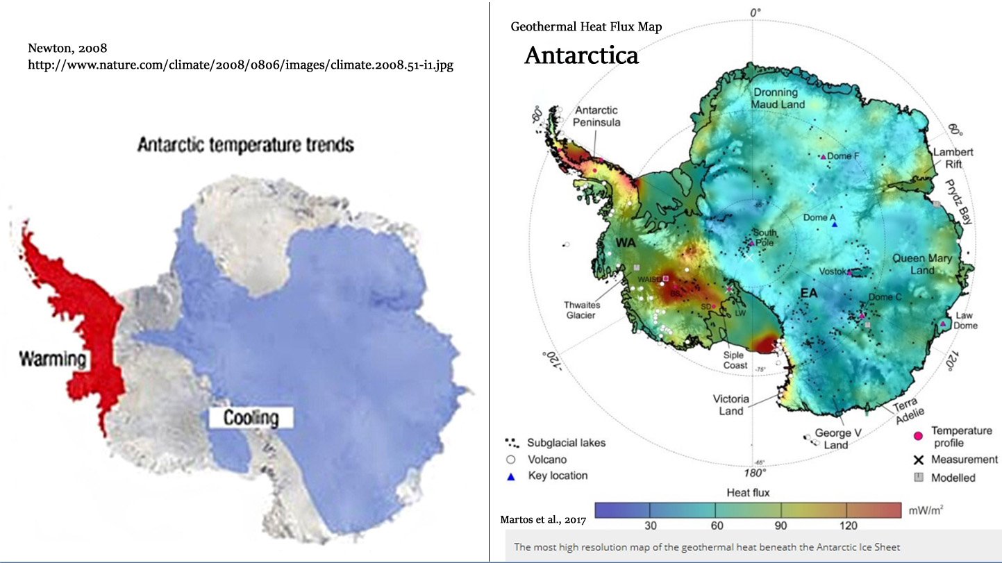
Iverson et al., 2017 The first physical evidence of subglacial volcanism under the West Antarctic Ice Sheet … New evidence from ice core tephra shows that subglacial volcanism can breach the surface of the ice sheet and may pose a great threat to WAIS stability. … The sources of these tephra layers were likely to be nearby subglacial volcanoes, Mt. Resnik, Mt. Thiel, and/or Mt. Casertz. A widespread increase in ice loss from WAIS could trigger positive feedback by decreasing ice mass and increasing decompression melting under the WAIS, increasing volcanism.
van Wyk de Vries et al., 2017 …in light of concerns over whether enhanced geothermal heat fluxes and subglacial melting may contribute to instability of the West Antarctic Ice Sheet. … The overall result presented here constitutes a first inventory of West Antarctica’s subglacial volcanism. We identified 138 volcanoes, 91 of which have not previously been identified, and which are widely distributed throughout the deep basins of West Antarctica, but are especially concentrated and orientated along the >3000 km central axis of the West Antarctic Rift System. … [V]olcanism affects geothermal heat flow and, hence, basal melting, potentially also impacting upon ice dynamics.
(press release) West Antarctica’s vast ice sheet conceals what may be the largest volcanic region on earth, research has revealed. … Previous studies and the concentration of volcanoes found in the region together suggest that activity may have occurred in previous warmer periods.
Recent Cooling In The North Atlantic, Southern Ocean (10)
Yeager and Robson, 2017 [W]hile the late twentieth century Atlantic was dominated by NAO-driven THC [thermohaline circulation] variability, other mechanisms may dominate in other time periods. … More recently, the SPNA [sub polar North Atlantic] upper ocean has again been cooling, which is also thought to be related to a slowdown in the THC. A continued near-term cooling of the SPNA has been forecast by a number of prediction systems, with implications for pan-Atlantic climate.
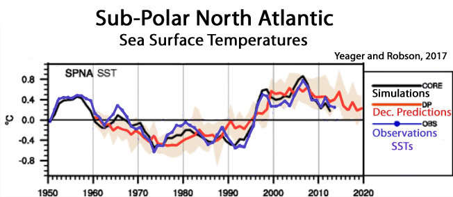
Latif et al., 2017 The Southern Ocean featured some remarkable changes during the recent decades. For example, large parts of the Southern Ocean, despite rapidly rising atmospheric greenhouse gas concentrations, depicted a surface cooling since the 1970s, whereas most of the planet has warmed considerably. In contrast, climate models generally simulate Southern Ocean surface warming when driven with observed historical radiative forcing. The mechanisms behind the surface cooling and other prominent changes in the Southern Ocean sector climate during the recent decades, such as expanding sea ice extent, abyssal warming, and CO2 uptake, are still under debate. Observational coverage is sparse, and records are short but rapidly growing, making the Southern Ocean climate system one of the least explored. It is thus difficult to separate current trends from underlying decadal to centennial scale variability.
Piecuch et al., 2017 The subpolar North Atlantic (SPNA) is subject to strong decadal variability, with implications for surface climate and its predictability. In 2004–2005, SPNA decadal upper ocean and sea-surface temperature trends reversed from warming during 1994–2004 to cooling over 2005–2015. … Over the last two decades, the SPNA has undergone a pronounced climate shift. Decadal OHC and SST trends reversed sign around 2004–2005, with a strong warming seen during 1994–2004 and marked cooling observed over 2005–2015. These trend reversals were pronounced (> 0.1 °C yr−1 in magnitude) in the northeastern North Atlantic (south and west of Iceland) and in the Labrador Sea. … To identify basic processes controlling SPNA thermal variations, we diagnose the SPNA heat budget using ECCOv4. Changes in the heat content of an oceanic control volume can be caused by convergences and divergences of advective, diffusive, and surface heat fluxes within the control volume. [Advective heat convergence] explains 87% of the total [ocean heat content] variance, the former [warming] showing similar decadal behavior to the latter [cooling], increasing over 1994–2004, and decreasing over 2005–2015. … These results demonstrate that the recent SPNA decadal trend reversal was mostly owing to advective convergences by ocean circulation … decadal variability during 1993–2015 is in largest part related to advection by horizontal gyres.
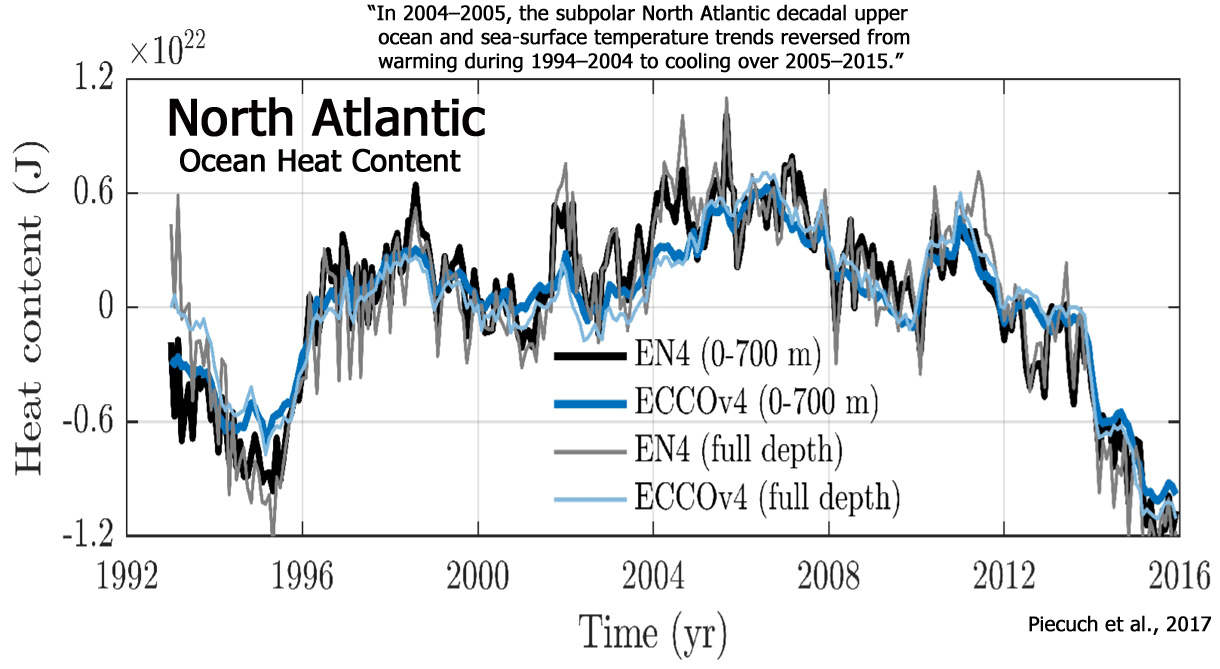
Li, 2017 In the Southern Ocean, the increasing trend of the total OHC slowed down and started to decrease from 1980, and it started to increase again after 1995. In the warming context over the whole period [1970-2009], the Pacific was losing heat, especially in the deep water below 1000 m and in the upper layer above 300 m, excluding the surface 20 m layer in which the OHC kept increasing through the time.
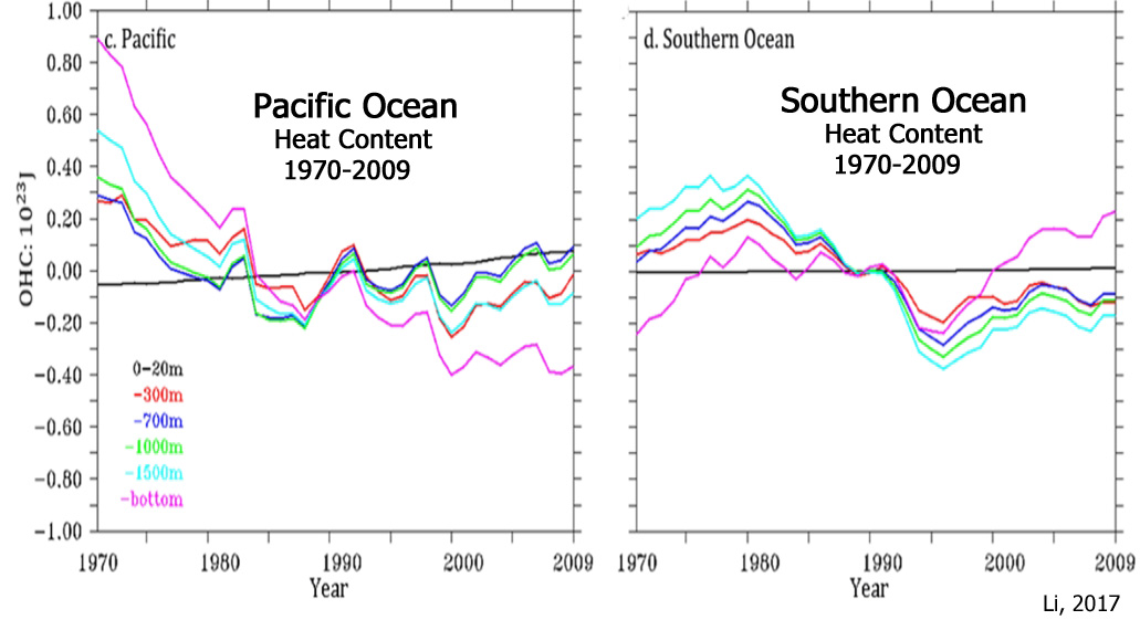
Kusahara et al., 2017 In contrast to a strong decrease in Arctic sea ice extent, overall Antarctic sea ice extent has modestly increased since 1979. Several hypotheses have been proposed for the net Antarctic sea ice expansion, including atmosphere/ocean circulation and temperature changes, sea ice-atmospheric-ocean feedback, increased precipitation, and enhanced basal meltwater from ice shelves. Concomitant with this positive trend in Antarctic sea ice, sea surface temperatures (SSTs) over the Southern Ocean south of approximately 45°S have cooled over this period [since 1979].
Turney et al., 2017 Occupying about 14% of the world’s surface, the Southern Ocean plays a fundamental role in ocean and atmosphere circulation, carbon cycling and Antarctic ice-sheet dynamics. … As a result of anomalies in the overlying wind, the surrounding waters are strongly influenced by variations in northward Ekman transport of cold fresh subantarctic surface water and anomalous fluxes of sensible and latent heat at the atmosphere–ocean interface. This has produced a cooling trend since 1979.
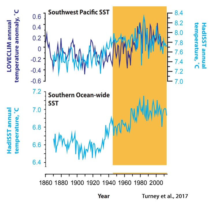
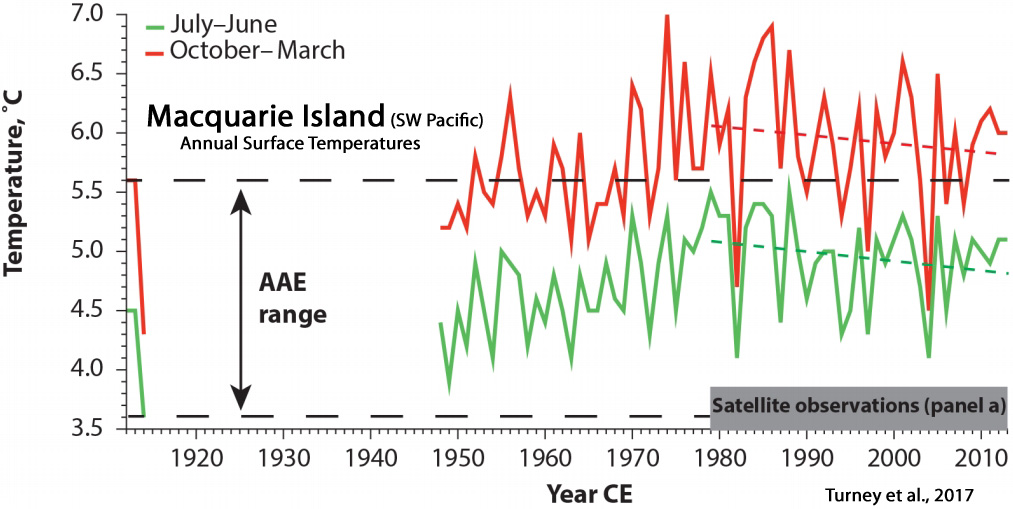
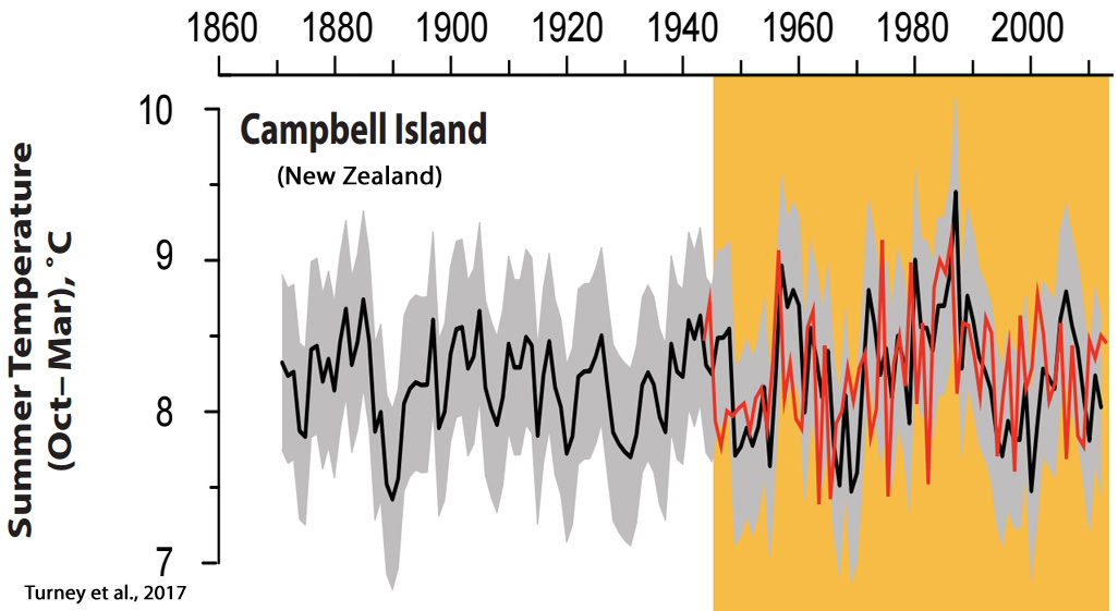
Kim et al., 2017

Gladyshev et al., 2017 After 2010, a sharp and stable freshening and cooling of SPMWs [Subpolar Mode Water] started in the eastern part of the North Atlantic. In the years 2010–2016, the mean temperature of the SPMW [Subpolar Mode Water] core in the Rockall Trough dropped by -0.73°C (-0.12°C/yr); in the Iceland Basin it dropped by -2.12°C (-0.35°C/yr), and salinity decreased by 0.12 psu (0.02 psu/yr) and 0.23 psu (0.04 psu/yr), respectively.
Yashayaev and Loder, 2017 As a result of this intermittent recurrence of intensified Labrador Sea Water formation, the annual average temperature and density in the region’s upper 2000m have predominantly varied on a bi-decadal time scale, rather than having a long-term trend as might be expected from anthropogenic climate change. … [I]ntermittent recurrence of enhanced deep convection periods in the Labrador Sea, and the associated formation of major LSW classes, are contributing to a predominant decadal-scale variation in hydrographic properties which makes it difficult to determine whether anthropogenic changes are occurring. … This strong, apparently natural, decadal-scale variability makes it very difficult to determine whether significant anthropogenic changes in LSW formation and properties have occurred.
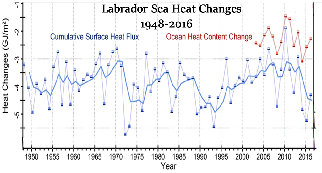

Robson et al., 2017 In the 1990s anomalously strong ocean heat transport convergence dominates the SPG [Subpolar Gyre, North Atlantic] warming. … The cooling of the SPG [Subpolar Gyre, North Atlantic] after 2005 is dominated by a reduction in ocean heat transport convergence, particularly in the eastern SPG. The reduced ocean heat transport is largely due to a weakening ocean circulation. By focusing on three independent case-studies of North Atlantic decadal change events the analysis presented here gives further support to the important role of ocean heat transport and ocean circulation in driving the observed changes in North Atlantic ocean heat content in the recent past.
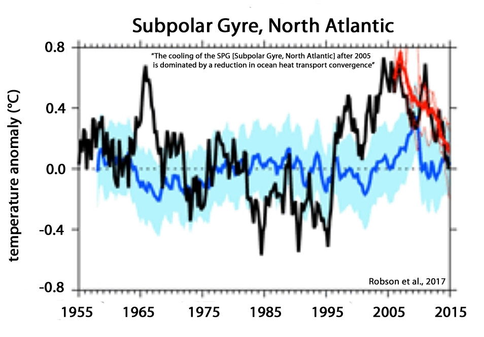


Recent Comments