1. Climate Change Observation, Reconstruction (190)
No Net Warming Since Mid/Late 20th Century (36)
A Warmer Past: Non-Hockey Stick Reconstructions (77)
Lack Of Anthropogenic/CO2 Signal In Sea Level Rise (16)
Sea Levels Multiple Meters Higher 4,000-7,000 Years Ago (18)
A Model-Defying Cryosphere, Polar Ice (34)
Mass Extinction Events Caused By Glaciation, Sea Level Fall (3)
Antarctic Ice Melting In High Geothermal Heat Flux Areas (2)
Abrupt, Degrees-Per-Decade Natural Global Warming (5)
No Net Warming Since The Mid/Late 20th Century
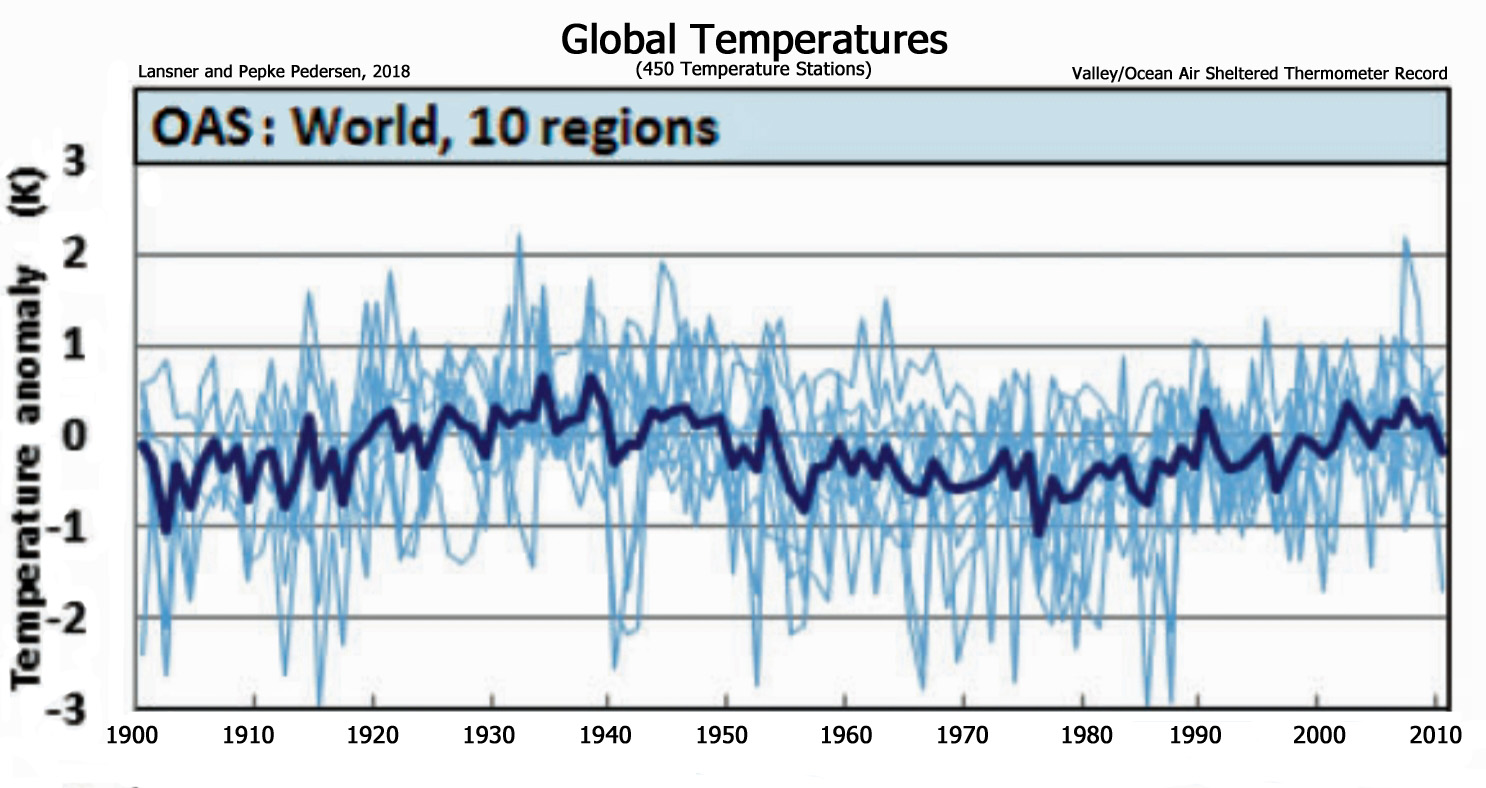
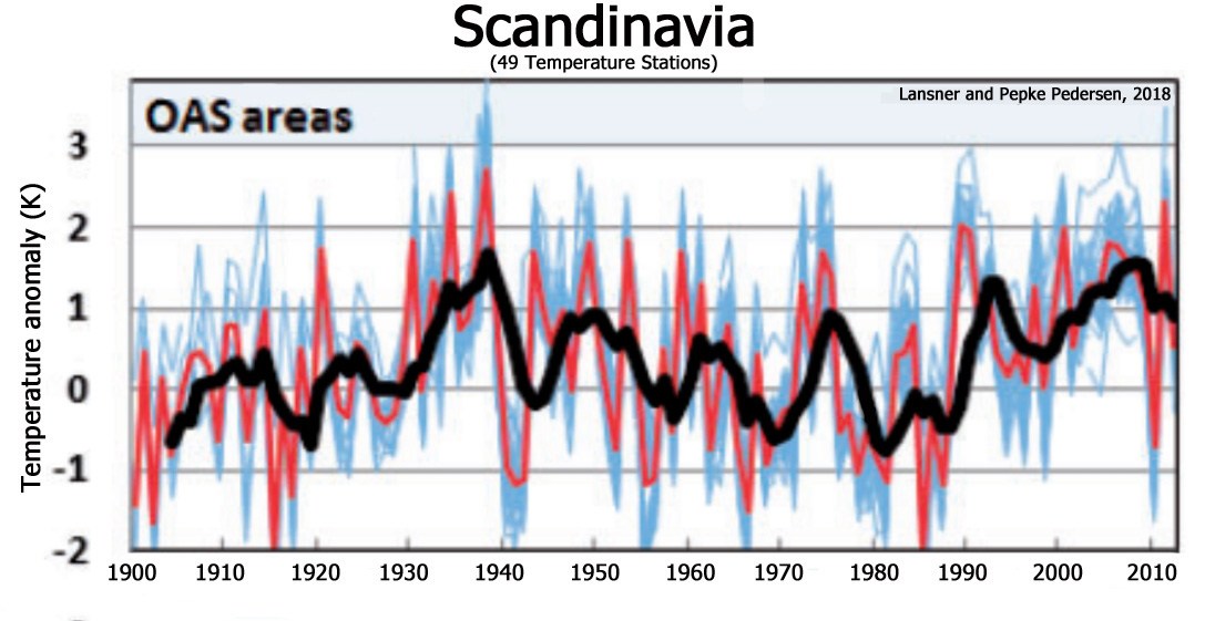
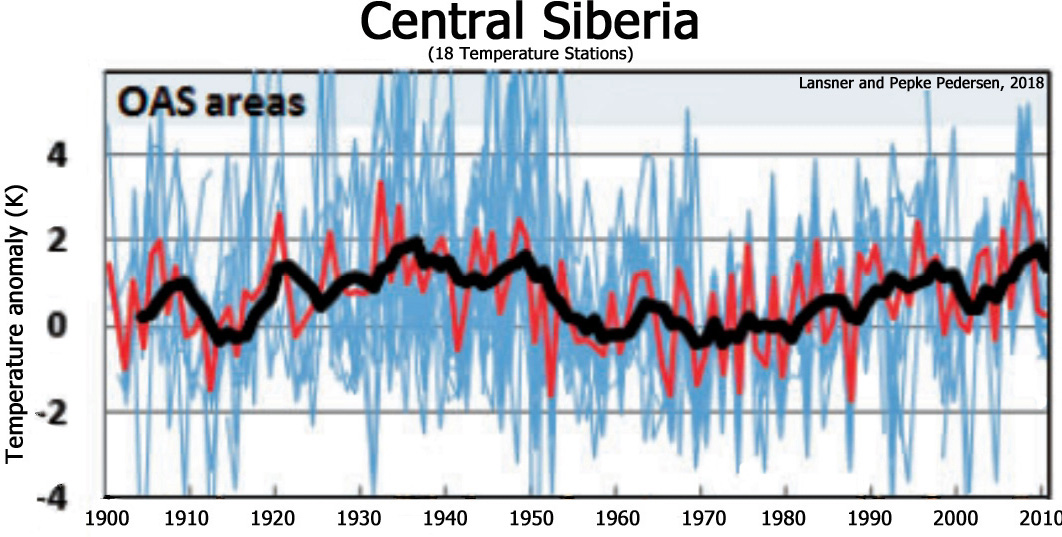
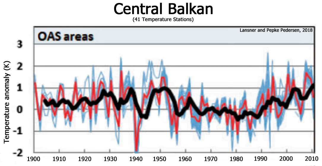
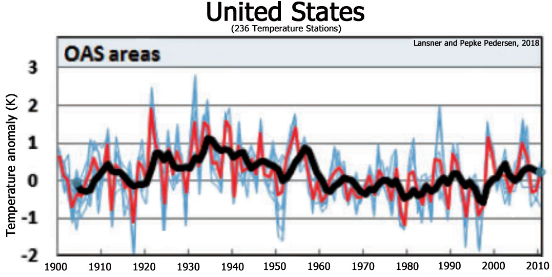
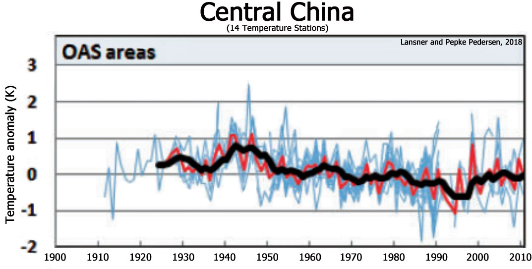
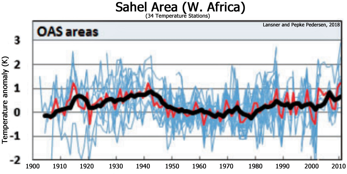
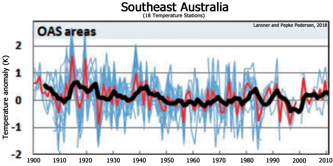
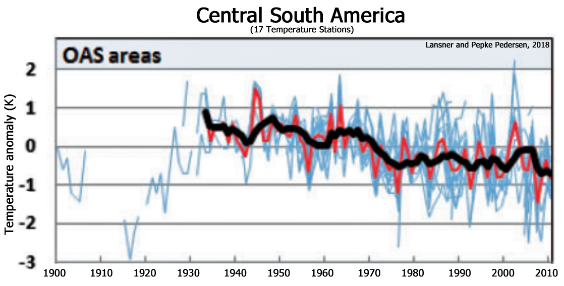
Lansner and Pepke Pedersen, 2018 In locations best sheltered and protected against ocean air influence, the vast majority of thermometers worldwide trends show temperatures in recent decades rather similar to the 1920–1950 period. This indicates that the present-day atmosphere and heat balance over the Earth cannot warm areas – typically valleys – worldwide in good shelter from ocean trends notably more than the atmosphere could in the 1920–1950 period. … [T]he lack of warming in the OAS temperature trends after 1950 should be considered when evaluating the climatic effects of changes in the Earth’s atmospheric trace amounts of greenhouse gasses as well as variations in solar conditions.


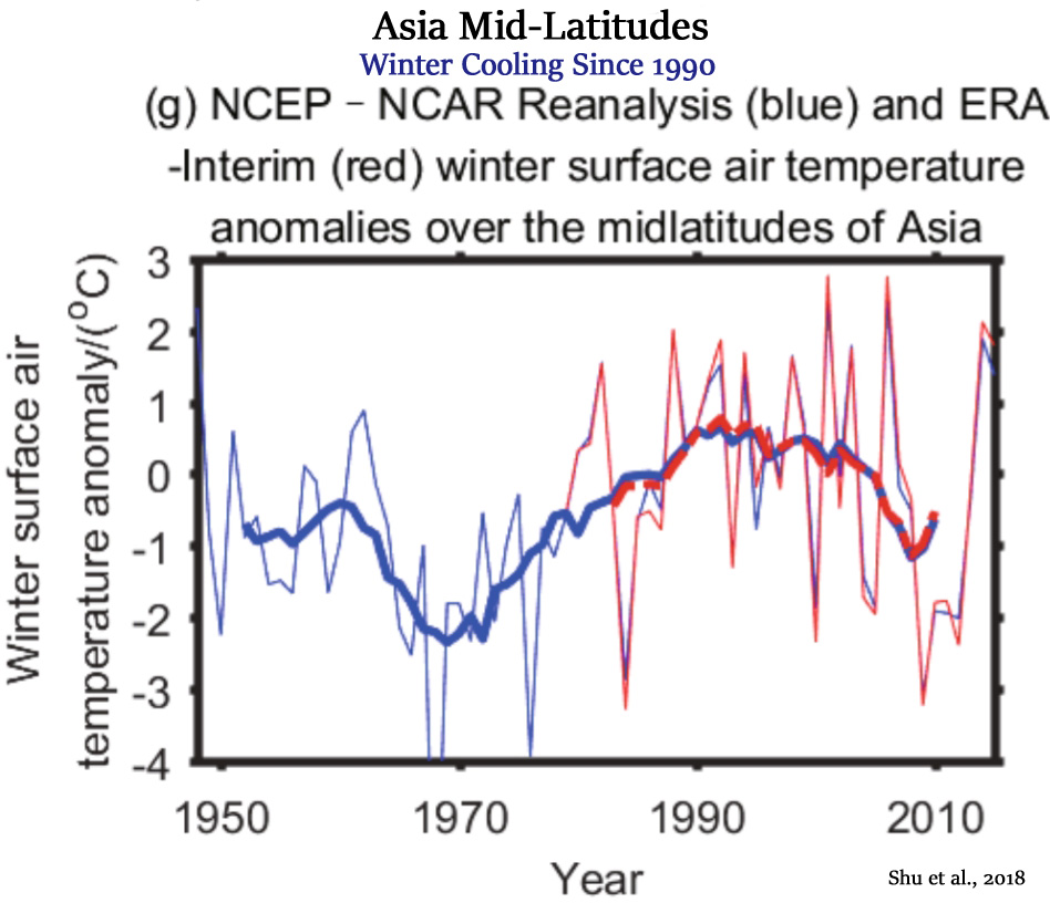
Shu et al., 2018 The link between boreal winter cooling over the midlatitudes of Asia and the Barents Oscillation (BO) since the late 1980s is discussed in this study, based on five datasets. Results indicate that there is a large-scale boreal winter cooling during 1990–2015 over the Asian midlatitudes, and that it is a part of the decadal oscillations of long-term surface air temperature (SAT) anomalies.
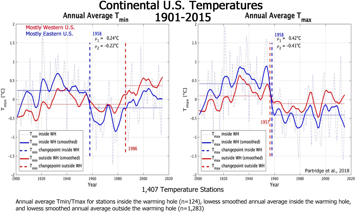
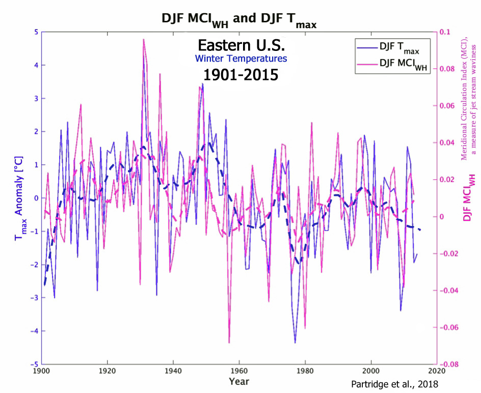
Partridge et al., 2018 We present a novel approach to characterize the spatiotemporal evolution of regional cooling across the eastern U.S. (commonly called the U.S. warming hole), by defining a spatially explicit boundary around the region of most persistent cooling. The warming hole emerges after a regime shift in 1958 where annual maximum (Tmax) and minimum (Tmin) temperatures decreased by 0.46°C and 0.83°C respectively. … [T]he seasonal modes also vary in causation. Winter temperatures in the warming hole are significantly correlated with the Meridional Circulation Index (MCI), North Atlantic Oscillation (NAO), and Pacific Decadal Oscillation (PDO). … We select only stations in the contiguous U.S. that have an 80% complete record from 1901-2015, resulting in 1407 temperature stations … [W]e note that there is considerable spatial coherence between the location of the summer warming hole and the region within which cooler extreme temperatures are associated with agricultural intensification (Mueller et al. 2015). Multiple studies have demonstrated that irrigation can have a significant influence on regional precipitation and can lead to cooler temperatures both locally through increased evapotranspiration, and downwind of the irrigated region through enhanced moisture transport (Alter et al., 2015; Bonfils & Lobell, 2007; Pei et al., 2014, 2016).

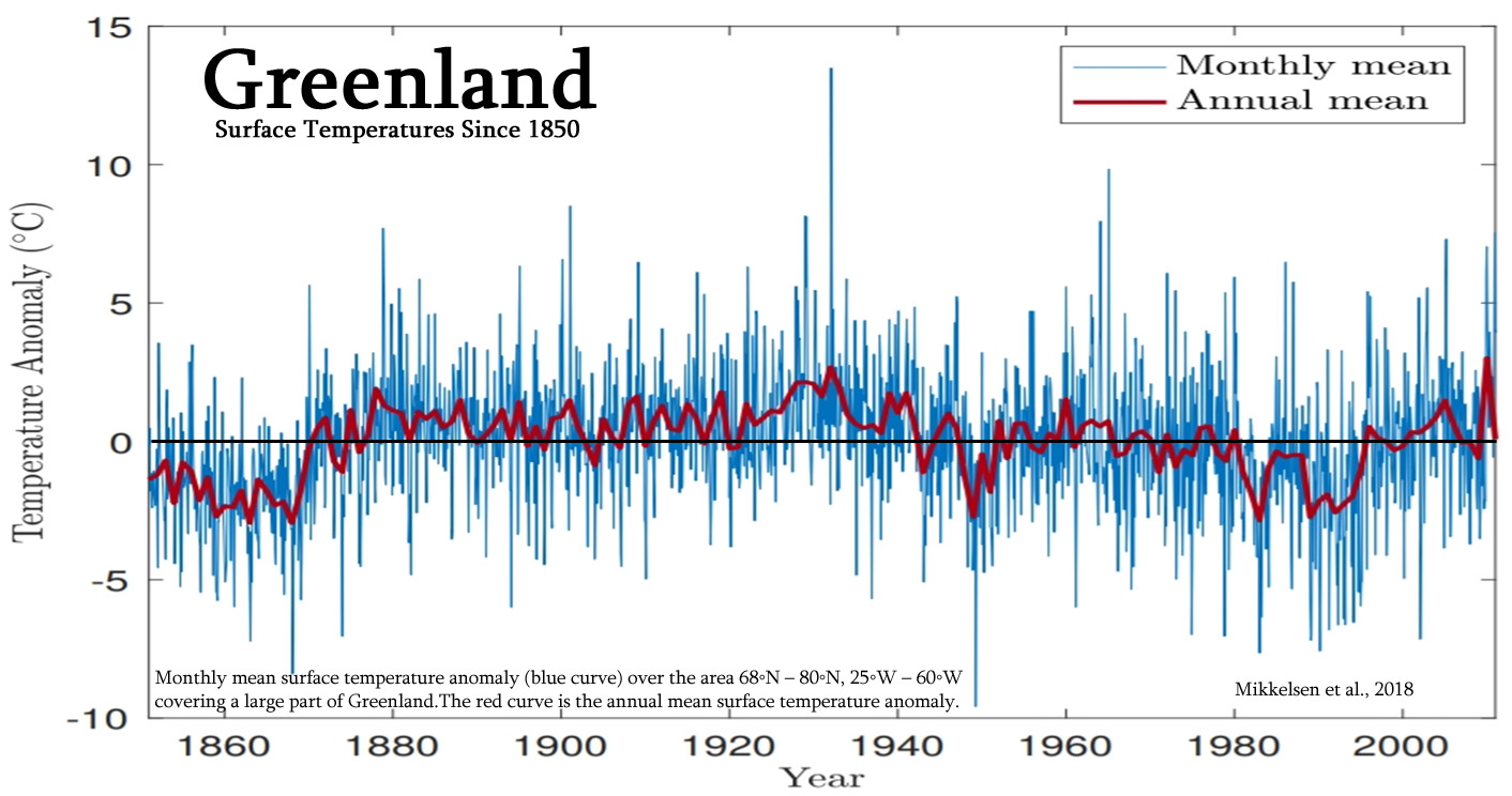
Mikkelsen et al., 2018
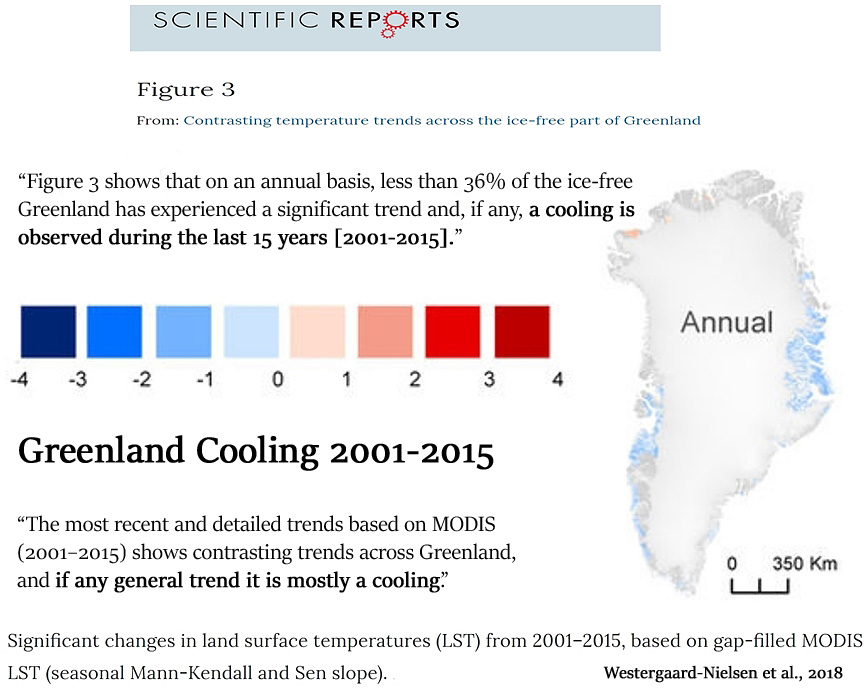
Westergaard-Nielsen et al., 2018 Here we quantify trends in satellite-derived land surface temperatures and modelled air temperatures, validated against observations, across the entire ice-free Greenland. … Warming trends observed from 1986–2016 across the ice-free Greenland is mainly related to warming in the 1990’s. The most recent and detailed trends based on MODIS (2001–2015) shows contrasting trends across Greenland, and if any general trend it is mostly a cooling. The MODIS dataset provides a unique detailed picture of spatiotemporally distributed changes during the last 15 years. … Figure 3 shows that on an annual basis, less than 36% of the ice-free Greenland has experienced a significant trend and, if any, a cooling is observed during the last 15 years (<0.15 °C change per year).
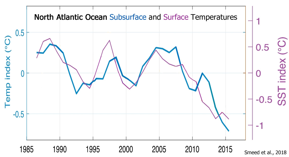
Smeed et al., 2018
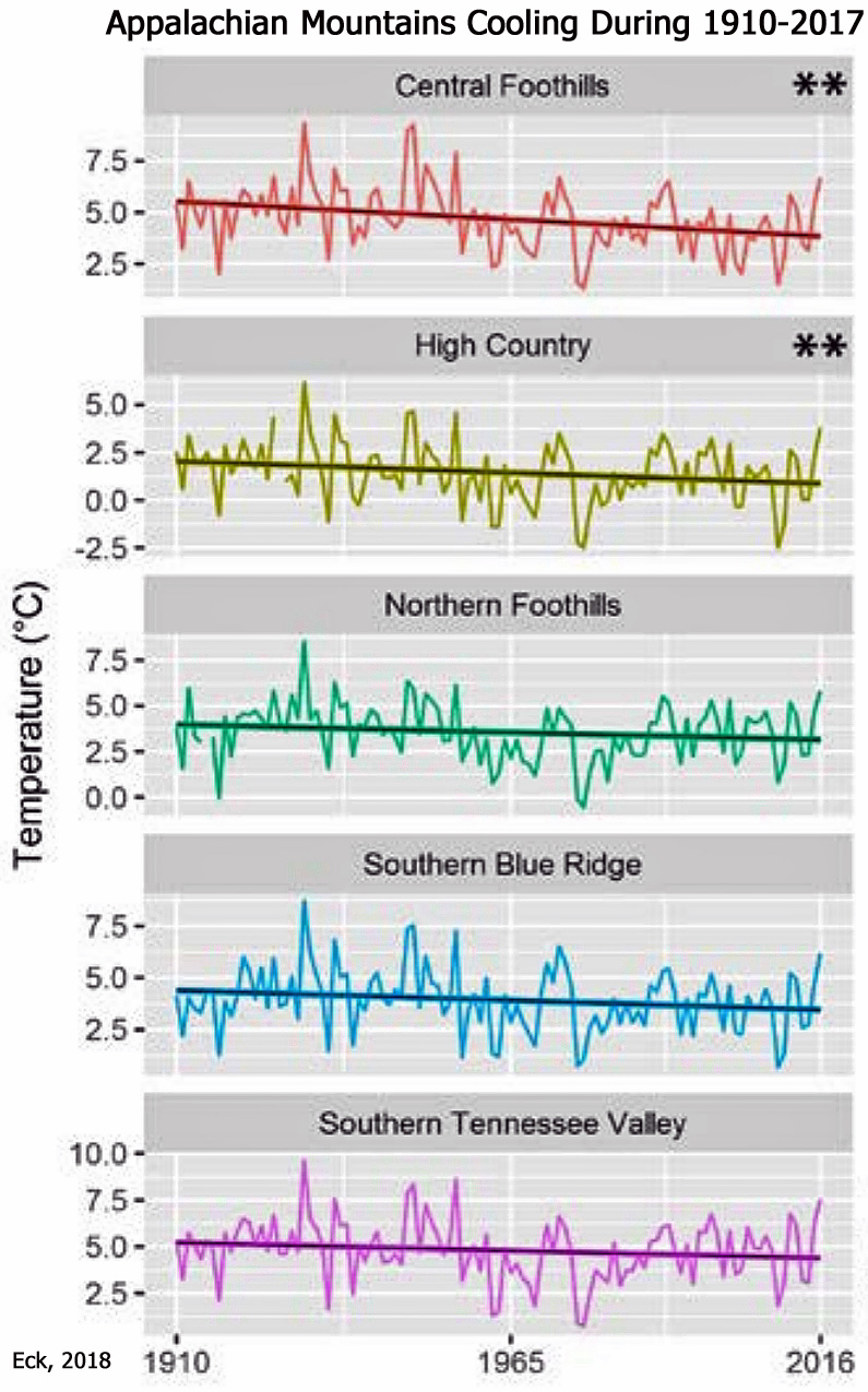
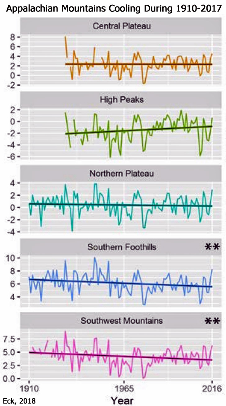
Eck, 2018 [A] majority (12/14) of the regions within the SAM [Southern Appalachian Mountains] have experienced a long-term decline in mean winter temperatures since 1910. Even after removing the highly anomalous 2009-2010 winter season, which was more than two standard deviations away from the long-term mean, the cooling of mean winter temperatures is still evident. … Higher winter temperatures dominated the early 20th century in the SAM [Southern Appalachian Mountains] with nine of the ten warmest winter seasons on record in the region having occurred before 1960. The 1931-1932 winter season, the warmest on record, averaged 8.0°C for DJF, nearly 4.7°C higher than the 1987-2017 normal mean winter temperature of 3.3°C. … Despite the 2016-2017 winter season finishing with the highest mean temperatures (5.7ºC) observed in the SAM [Southern Appalachian Mountains] since 1956-1957, there have been several years of anomalous negative temperature anomalies, with the 2009-2010 (0.3ºC) and 2010-2011 (1.2ºC) winter seasons finishing as two of the coldest on record for all regions.

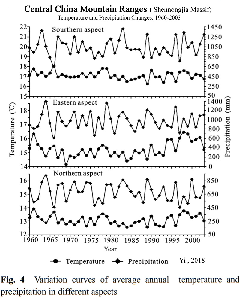
Yi, 2018 As measures of climate response, temperature and precipitation data from the north, east, and south-facing mountain ranges of Shennongjia Massif in the coldest and hottest months (January and July), different seasons (spring, summer, autumn, and winter) and each year were analyzed from a long-term dataset (1960 to 2003) to tested variations characteristics, temporal and spatial quantitative relationships of climates. The results showed that the average seasonal temperatures and precipitation in the north, east, and south aspects of the mountain ranges changed at different rates. The average seasonal temperatures change rate ranges in the north, east, and south-facing mountain ranges were from –0.0210 ℃/yr to 0.0143 ℃/yr, –0.0166 ℃/yr to 0.0311 ℃/yr, and –0.0290 ℃/yr to 0.0084 ℃/yr, respectively, and seasonal precipitation variation magnitude were from –1.4940 mm/yr to 0.6217 mm/yr, –1.6833 mm/yr to 2.6182 mm/yr, and –0.8567 mm/yr to 1.4077 mm/yr, respectively. The climates variation trend among the three mountain ranges were different in magnitude and direction, showing a complicated change of the climates in mountain ranges and some inconsistency with general trends in global climate change.
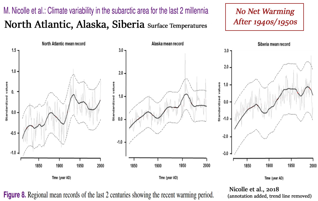
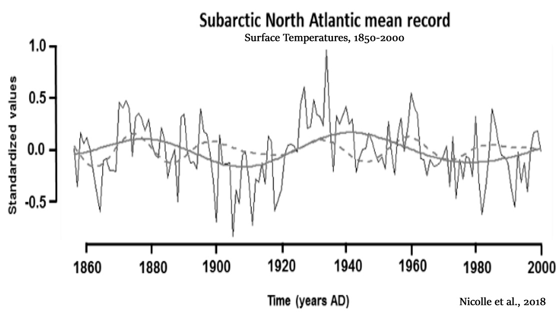
Nicolle et al., 2018 Persistent multidecadal variability with a period of 50– 90 years is consistent between the subarctic North Atlantic mean record and the AMO over the last 2 centuries (AD 1856–2000). … The climate of the Arctic–subarctic is influenced by the Atlantic and the Pacific oceans, which experience internal variability on different timescales with specific regional climate impacts. In the North Atlantic sector, instrumental sea surface temperature (SST) variations since AD 1860 highlight low-frequency oscillations known as the AMO (Kerr, 2000). … The evidence of industrial era warming starting earlier at the beginning of the 19th century was proposed by Abram et al. (2016) for the entire Arctic area. However, the intense volcanic activity of the 19th century (1809, 1815 and around 1840; Sigl et al., 2015) may also explain the apparent early warming trend, suggesting that it may have been recovery from an exceptionally cool phase. On the scale of the Holocene, internal fluctuations occurring on a millennial scale have been identified in the subarctic North Atlantic area and were tentatively related to ocean dynamics (Debret et al., 2007; Mjell et al., 2015). … The LIA is, however, characterized by an important spatial and temporal variability, particularly visible on a more regional scale (e.g., PAGES 2k Consortium, 2013). It has been attributed to a combination of natural external forcings (solar activity and large volcanic eruptions) and internal sea ice and ocean feedback, which fostered long-standing effects of short-lived volcanic events (Miller et al., 2012).
Purich et al., 2018 Observed Southern Ocean changes over recent decades include a surface freshening (Durack and Wijffels 2010; Durack et al. 2012; de Lavergne et al. 2014), surface cooling (Fan et al. 2014; Marshall et al. 2014; Armour et al. 2016; Purich et al. 2016a) and circumpolar increase in Antarctic sea ice (Cavalieri and Parkinson 2008; Comiso and Nishio 2008; Parkinson and Cavalieri 2012). … [A]s high-latitude surface freshening is associated with surface cooling and a sea ice increase, this may be another factor contributing to the CMIP5 models excessive Southern Ocean surface warming contrasting the observed surface cooling (Marshall et al. 2014; Purich et al. 2016a), and sea ice decline contrasting the observed increases (Mahlstein et al. 2013; Polvani and Smith 2013; Swart and Fyfe 2013; Turner et al. 2013; Zunz et al. 2013; Gagne et al. 2015) over recent decades. … Our results suggest that recent multi-decadal trends in large-scale surface salinity over the Southern Ocean have played a role in the observed surface cooling seen in this region. … The majority of CMIP5 models do not simulate a surface cooling and increase in sea ice (Fig. 8b), as seen in observations.
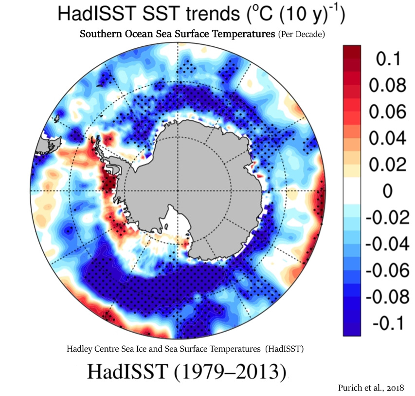
Cerrone and Fusco, 2018 Compelling evidence indicates that the large increase in the SH sea ice, recorded over recent years, arises from the impact of climate modes and their long-term trends. The examination of variability ranging from seasonal to interdecadal scales, and of trends within the climate patterns and total Antarctic sea ice concentration (SIC) for the 32-yr period (1982–2013), is the key focus of this paper. The results herein indicate that a progressive cooling has affected the year-to-year climate of the sub-Antarctic since the 1990s. This feature is found in association with increased positive SAM and SAO phases detected in terms of upward annual and seasonal trends (in autumn and summer) and upward decadal trends. In addition, the SIC [sea ice concentration] shows upward annual, spring, and summer trends, indicating the insulation of Antarctica from the warmer flows in the midlatitudes.
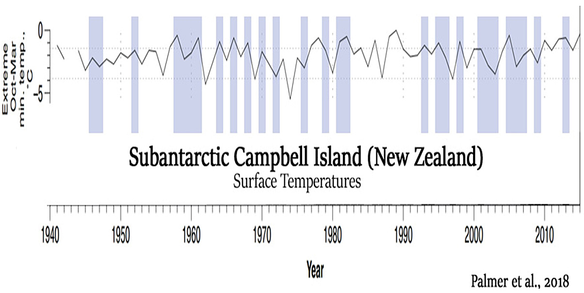
Palmer et al., 2018
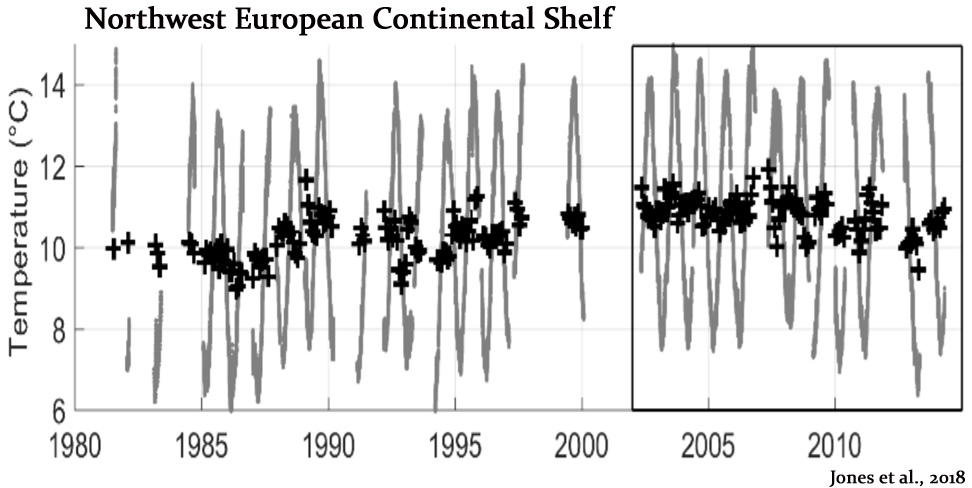
Jones et al., 2018
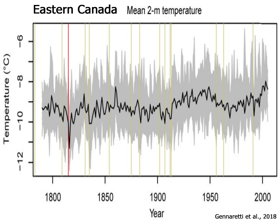
Gennaretti et al., 2018
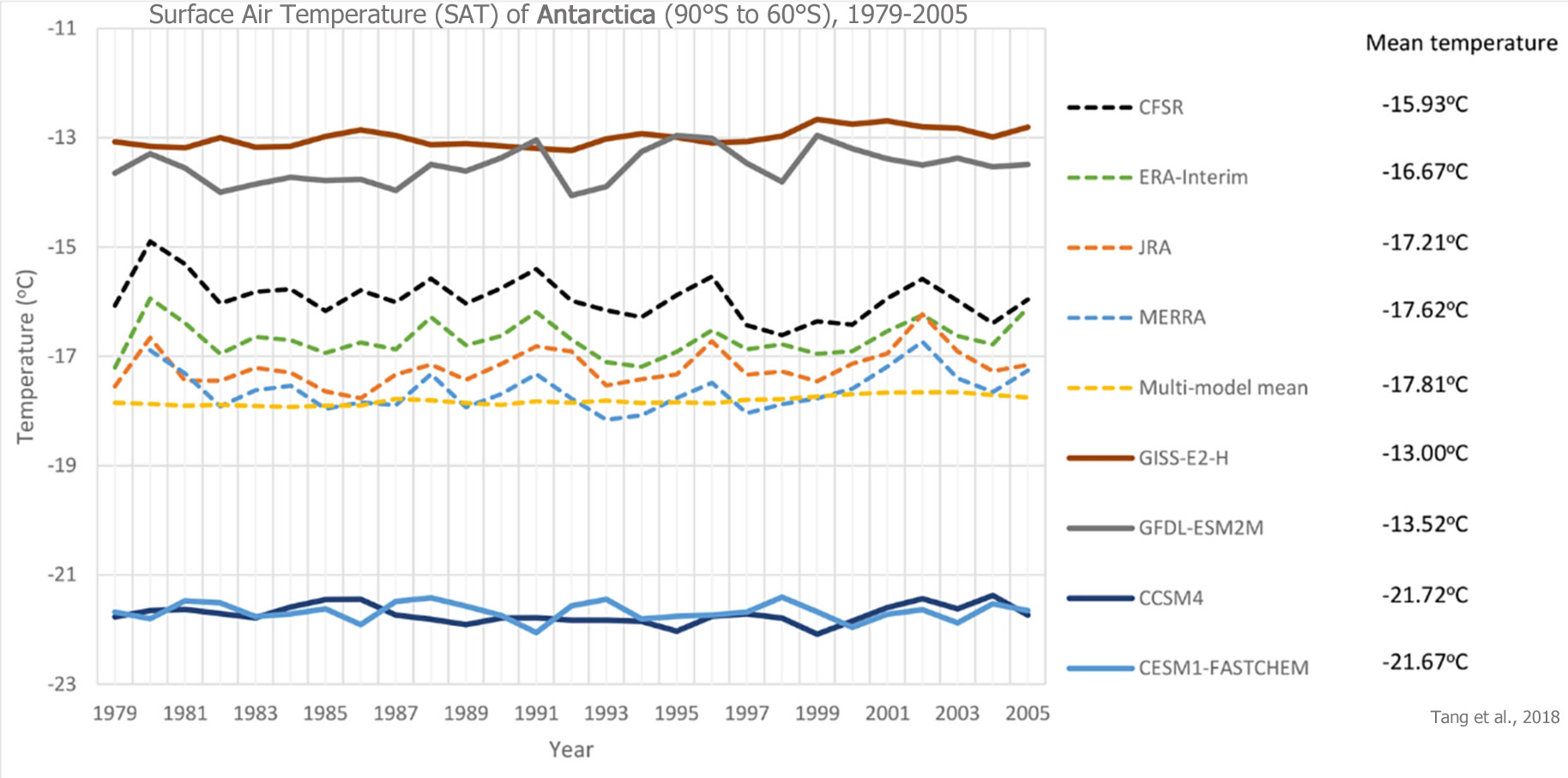
Tang et al., 2018 The study of Antarctic precipitation has attracted a lot of attention recently. The reliability of climate models in simulating Antarctic precipitation, however, is still debatable. This work assess the precipitation and surface air temperature (SAT) of Antarctica (90°S to 60°S) using 49 Coupled Model Intercomparison Project phase 5 (CMIP5) global climate models
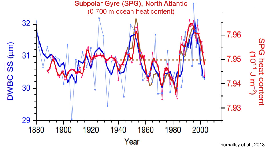
Thornalley et al., 2018
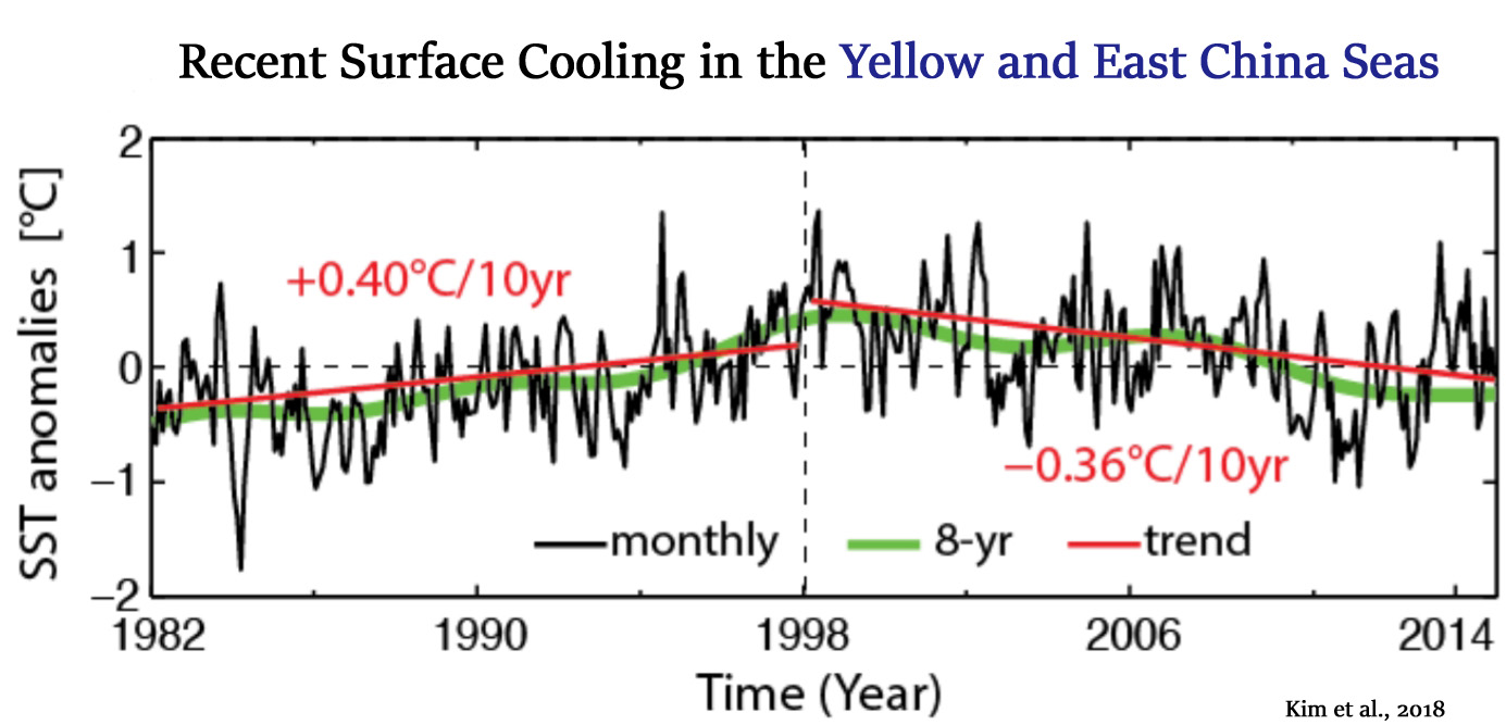
Kim et al., 2018 Recent surface cooling in the Yellow and East China Seas and the associated North Pacific climate regime shift … The Yellow and East China Seas (YECS) are widely believed to have experienced robust, basin-scale warming over the last few decades. However, the warming reached a peak in the late 1990s, followed by a significant cooling trend. … The most striking evolution pattern is that a robust warming trend at a rate of +0.40°C per decade reached a peak in the late 1990s, and then it turned downward at a rate of −0.36°C per decade. The positive and then negative trends are estimated throughout the YECS for the periods 1982−1997.
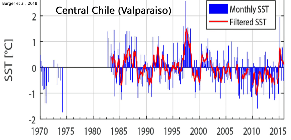
Burger et al., 2018 Previous studies have identified spatial and temporal trends in temperature and precipitation in Chile over recent decades. Temperature rose significantly during the mid to late 20th century in coastal locations between 18 to 33 °S (Rosenblüth et al., 1997), but then started to decrease, with a cooling trend up to -0.20ºC decade-1 dominating over the past 20-30 years (Falvey and Garreaud, 2009).
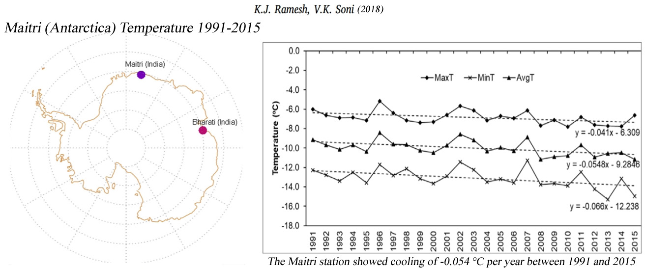
Ramesh and Soni, 2018 The present paper reviews the progress of India’s scientific research in polar meteorology. The analysis of 25 years meteorological data collected at Maitri station for the period 1991–2015 is presented in the paper. The observed trend in thetemperature data of 19 Antarctic stations obtained from READER project for the period 1991–2015 has also been examined. The 25 years long term temperature record shows cooling over Maitri station. The Maitri station showed cooling of 0.054 °C per year between 1991 and 2015, with similar pronounced seasonal trends. The nearby Russian station Novolazarevskaya also showed a cooling trend of 0.032 °C per year. … The temperature trend in average temperature of 19 Antarctica stations is also examined to ascertain the extent of cooling or warming trend (Supplementary Table_S1). The majority of stations in East Antarctica close to the coast show cooling or no significant trend. … Turner et al. (2016) using stacked temperature record found a significant cooling trend for the Antarctic Peninsula for the period 1999–2014.
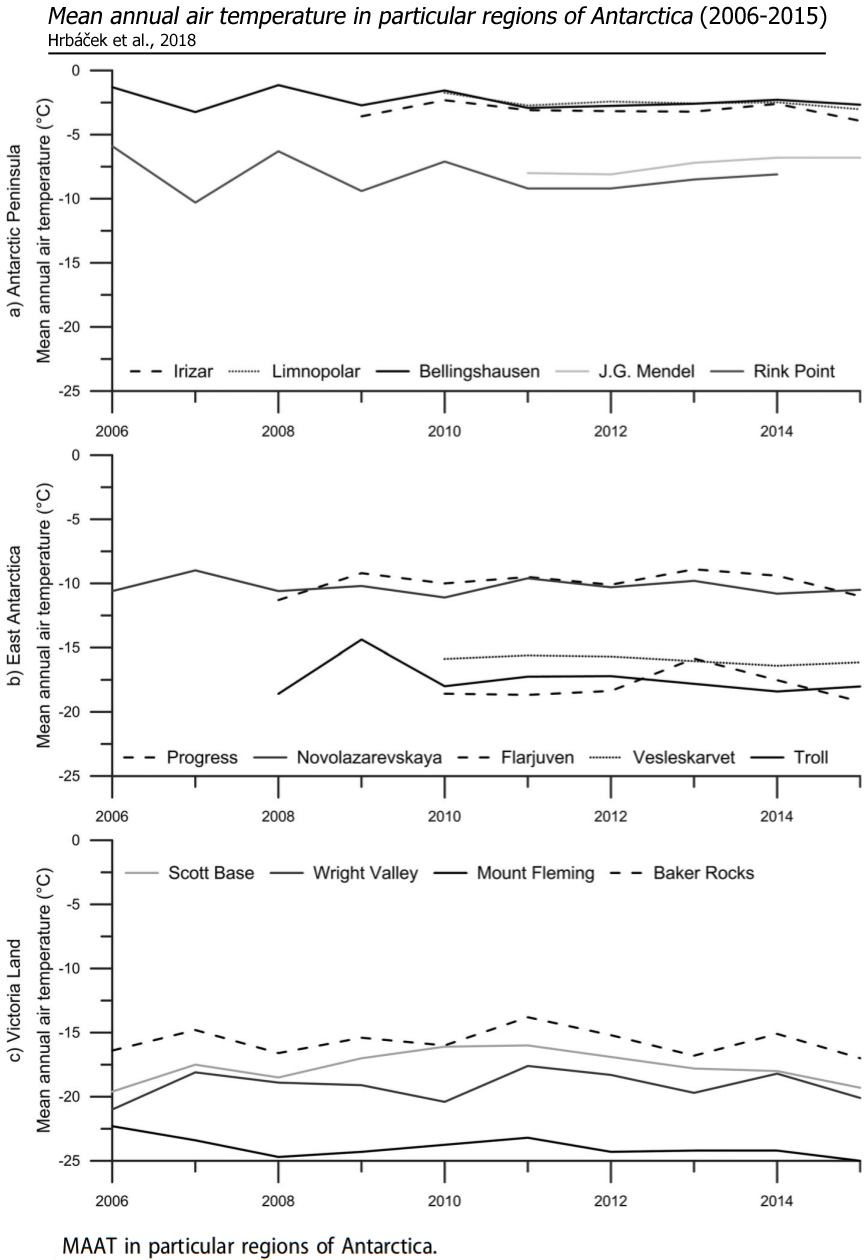
Hrbáček et al., 2018 Active layer monitoring in Antarctica: an overview of results from 2006 to 2015 … Air temperatures showed significant regional differences within the study areas. In the western Antarctic Peninsula region, Vestfold Hills and northern Victoria Land, a slight air temperature cooling was detected, while at other sites in Victoria Land and East Antarctica the air temperature was more irregular, showing no strong overall trend of warming or cooling during the study period (Figure 2). The Antarctic Peninsula region has been reported as the most rapidly warming part of Antarctica (e.g. Turner et al., 2005, 2014), but cooling has been reported since 2000 (Turner et al., 2016). Relatively stable air temperature conditions during the past 20 years were reported in Victoria Land (Guglielmin & Cannone, 2012).
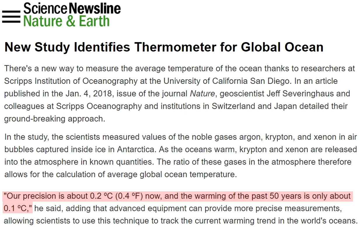
Bereiter et al., 2018 Our reconstruction provides unprecedented precision and temporal resolution for the integrated global ocean, in contrast to the depth-, region-, organism- and season-specific estimates provided by other methods. We find that the mean global ocean temperature is closely correlated with Antarctic temperature and has no lead or lag with atmospheric CO2, thereby confirming the important role of Southern Hemisphere climate in global climate trends. We also reveal an enigmatic 700-year warming during the early Younger Dryas period (about 12,000 years ago) that surpasses estimates of modern ocean heat uptake.

(press release) “Our precision is about 0.2 ºC (0.4 ºF) now, and the warming of the past 50 years is only about 0.1 ºC,” he said, adding that advanced equipment can provide more precise measurements, allowing scientists to use this technique to track the current warming trend in the world’s oceans.
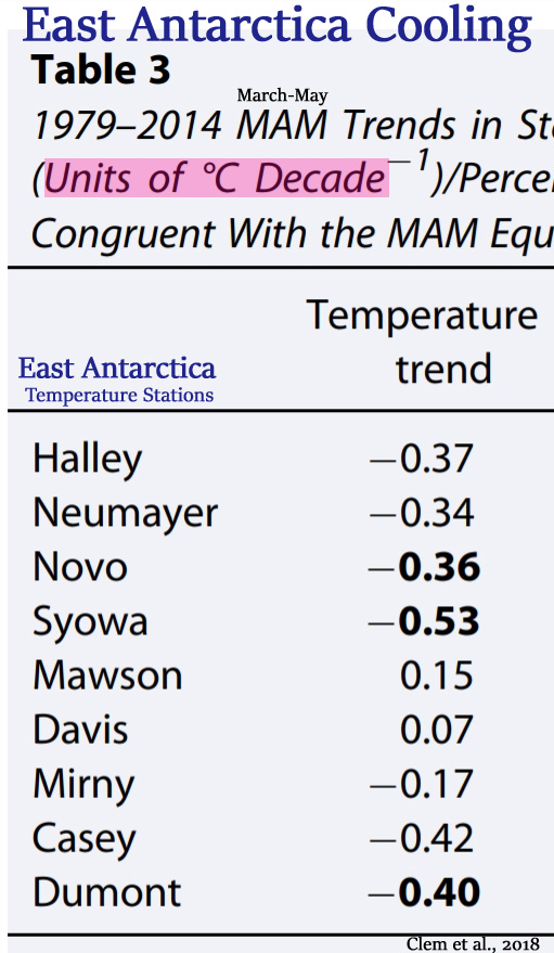
Clem et al., 2018 Over the past 60 years [since 1957], the climate of East Antarctica cooled while portions of West Antarctica were among the most rapidly warming regions on the planet. The East Antarctic cooling is attributed to a positive trend in the Southern Annular Mode (SAM) and a strengthening of the westerlies, while West Antarctic warming is tied to zonally asymmetric circulation changes forced by the tropics. [CO2 is not mentioned in the paper as a factor in warming/cooling trends.] This study finds recent (post-1979) surface cooling of East Antarctica during austral autumn to also be tied to tropical forcing, namely, an increase in La Niña events. … The South Atlantic anticyclone is associated with cold air advection, weakened northerlies, and increased sea ice concentrations across the western East Antarctic coast, which has increased the rate of cooling at Novolazarevskaya and Syowa stations after 1979. This enhanced cooling over western East Antarctica is tied more broadly to a zonally asymmetric temperature trend pattern across East Antarctica during autumn that is consistent with a tropically forced Rossby wave rather than a SAM pattern; the positive SAM pattern is associated with ubiquitous cooling across East Antarctica.
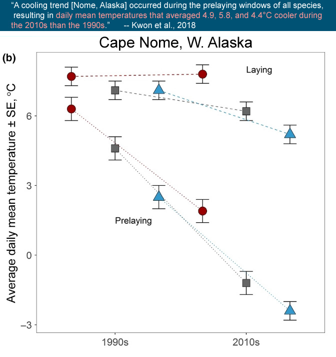
Kwon et al., 2018 We monitored 1,378 nests of western sandpipers, semipalmated sandpipers, and red‐necked phalaropes at a subarctic site during 1993–1996 and 2010–2014. … We found an unexpected long‐term cooling trend during the early part of the breeding season. Three species delayed clutch initiation by 5 days in the 2010s relative to the 1990s. … A cooling trend occurred during the prelaying windows of all species, resulting in daily mean temperatures that averaged 4.9, 5.8, and 4.4°C cooler during the 2010s than the 1990s for western sandpiper, semipalmated sandpiper, and red‐necked phalaropes, respectively.
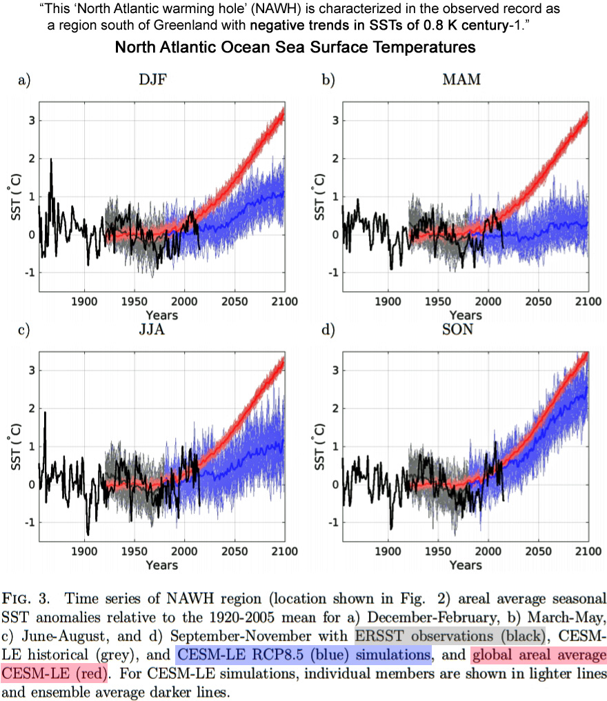
Gervais et al., 2018 Recent studies have documented the development of a warming deficit in North Atlantic sea surface temperatures (SST) both in observations of the current climate (Rahmstorf et al. 2015; Drijfhout et al. 2012) and in future climate simulations (Drijfhout et al. 2012; Marshall et al. 2015; Woollings et al. 2012). This “North Atlantic warming hole” (NAWH) is characterized in the observed record as a region south of Greenland with negative trends in SSTs [cooling] of 0.8 K century-1 (Rahmstorf et al. 2015). In fully coupled global climate model (GCM) future simulations, the NAWH is seen as a significant deficit in warming within the North Atlantic subpolar gyre (Marshall et al. 2015; Winton et al. 2013; Gervais et al. 2016). This local reduction in future warming is communicated to the overlying atmosphere and may impact atmospheric circulation (Gervais et al. 2016), including the North Atlantic storm track (Woollings et al. 2012).
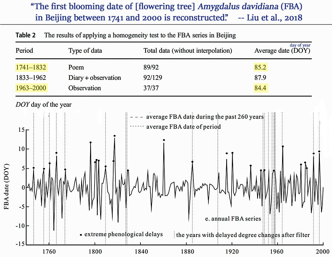
Liu et al., 2018 Plant phenology is an important natural indicator of climate change (Körner and Basler 2010) and a proxy for climate reconstruction (Ge et al. 2008; Zheng et al. 2015; Fang and Chen 2015). … In this paper, we reconstruct a phenological series of the first blooming date of Amygdalus davidiana (FBA) in Beijing from A.D. 1741 to 2000. In these series, phenological records after 1950 are all observational data, and before that are reconstructed data based on the records from diaries, poems and other historical documents. In China, poems and diaries are used as important sources of proxy data for reconstructing historical phenological series (Ge et al. 2008) because many phenological phenomena had been recorded in detail in these historical documents (Chuine et al. 2004; Zhang et al. 2013; Liu et al. 2016). … Based on the average of the FBA series, the original FBA series could be divided into 1 later blooming periods of A.D. 1796–1985 and 2 earlier blooming periods of A.D. 1741–1795 and A.D. 1985–2000. … Approximately 85% of the extreme delays followed the large volcanic eruptions (VEI ≥ 4), as the same proportion of the extreme delays followed El Niño events. About 73% of the extreme delays fall in the valleys of sunspot cycles or the Dalton minimum period in the year or the previous year.
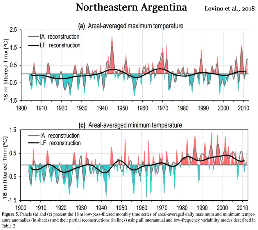
Lovino et al., 2018
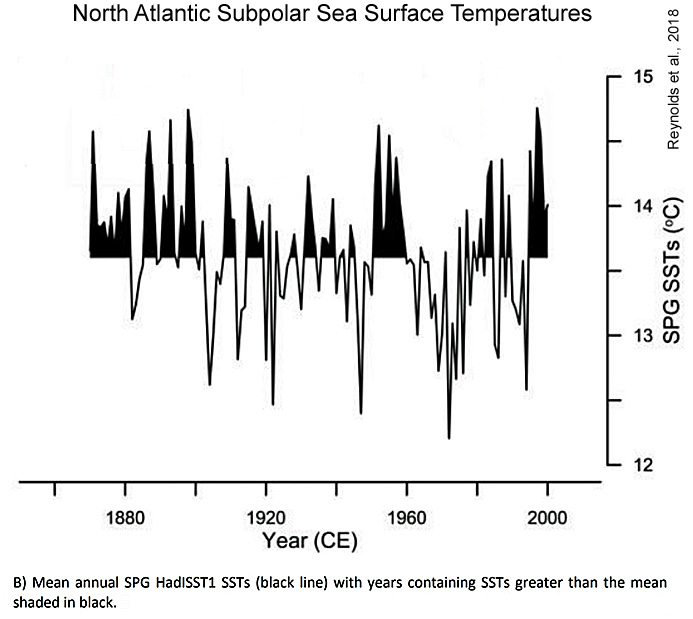
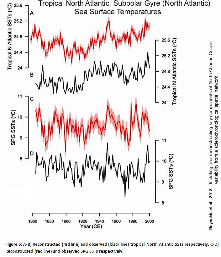
Reynolds et al., 2018
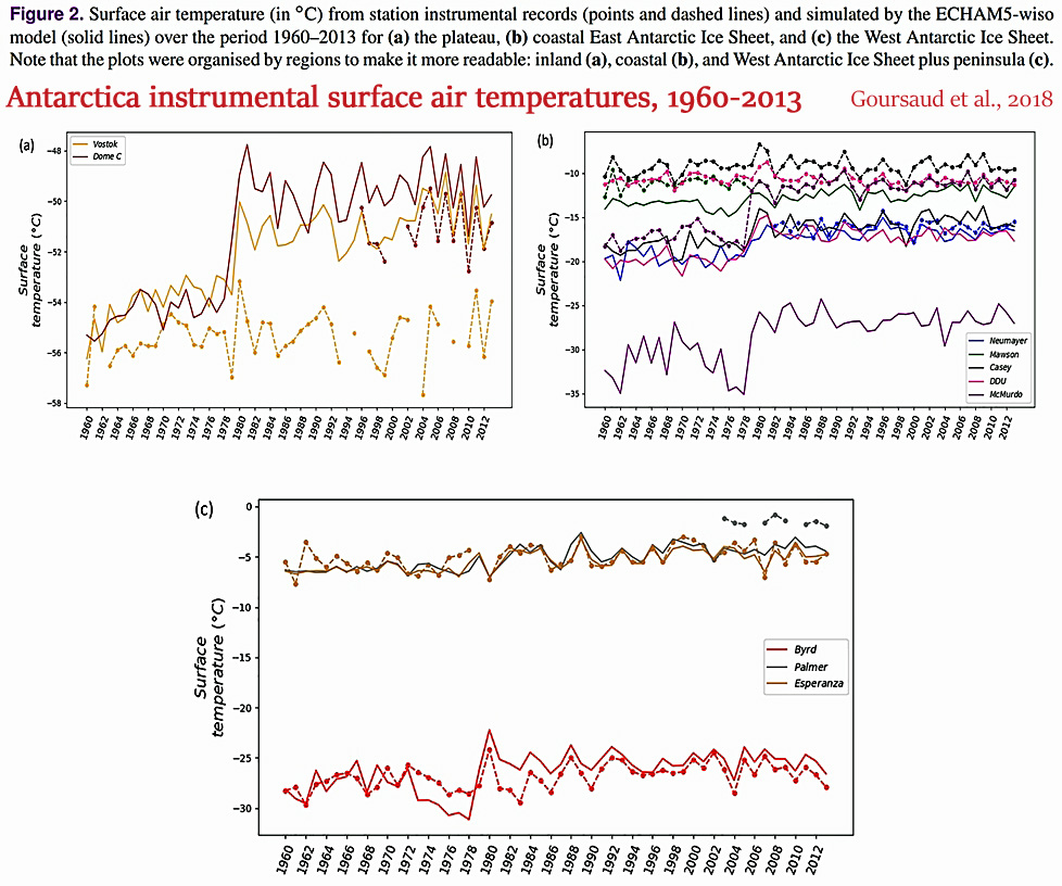
Goursaud et al., 2018
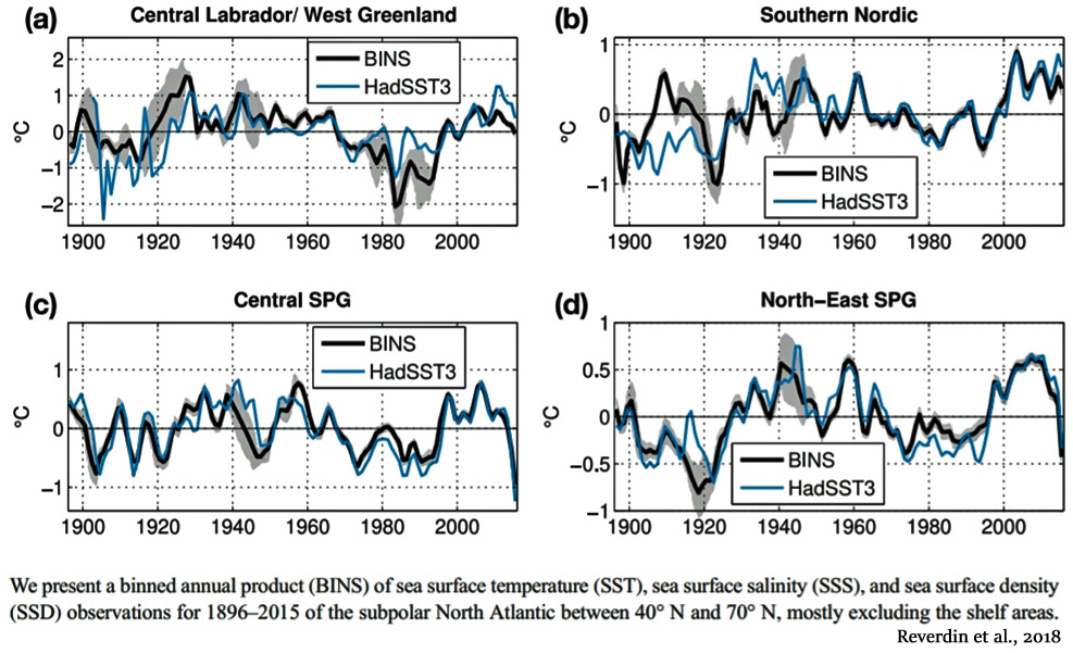
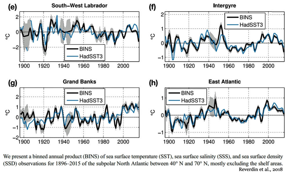
Reverdin et al., 2018
Dahal et al., 2018 (Illinois, USA) Illinois ranks either first or second in soybean production and second in corn production among the Midwestern states, with more than 75% of its land used for crop production. Agriculture defines the economy and the social structure of the state. Any changes in climate, temperature and rainfall is expected to affect the Midwestern states and their agricultural productivity. This study shows us that the climate change has not yet manifested itself in the state of Illinois. Any changes in temperature observed in the last 60 years have only helped towards catalyzing the agricultural productivity. Most of the stations of the state do not show significant change in the temperature parameters. Among those stations where the change is significant, the majority show a cooling trend. It was especially significant agriculturally that the summer days show cooling effect. This would imply a decreasing exposure of the crops to heat stresses. Also, it was significant that the range between the maximum and minimum daily temperature is narrowing and the average temperature is shifting towards the warmer domain without getting extreme. Thus, we can safely conclude that over the second half of the twentieth century, the temperature has shown characteristics that are very encouraging for the farmers of Illinois.
Lei et al.,2018 (N, NE, SE China) The authors analyzed the observed winter surface air temperature in eastern mainland China during the recent global warming hiatus period through 1998-2013. The results suggest a substantial cooling trend of about -1.0°/decade in Eastern China, Northeast China and Southeast China.
Cerrone and Fusco, 2018 (Antarctica) Compelling evidence indicates that the large increase in the SH sea ice, recorded over recent years, arises from the impact of climate modes and their long-term trends. The examination of variability ranging from seasonal to interdecadal scales, and of trends within the climate patterns and total Antarctic sea ice concentration (SIC) for the 32-yr period (1982–2013), is the key focus of this paper. The results herein indicate that a progressive cooling has affected the year-to-year climate of the sub-Antarctic since the 1990s.
Fernandoy et al., 2018 (Antarctic Peninsula) As shown by firn core analysis, the near-surface temperature in the northern-most portion of the Antarctic Peninsula shows a decreasing trend (−0.33°C year−1) between 2008 and 2014 [-1.98°C].
Vignon et al., 2018 (Antarctica) The near‐surface Antarctic atmosphere experienced significant changes during the last decades (Steig et al., 2009; Turner et al., 2006). In particular, the near‐surface air over the Western part of Antarctica exhibits one of the major warming over the globe (Bromwich et al., 2013a), with heating rates larger than 0.5 K per decade at some places. Despite a significant warming in the end of the 20th century, the Antarctic Peninsula has been slightly cooling since 1998, reflecting the high natural variability of the climate in this region (Turner et al., 2016). East Antarctica has experienced a slight cooling trend (Nicolas & Bromwich, 2014; Smith & Polvani, 2017) particularly marked during autumn.
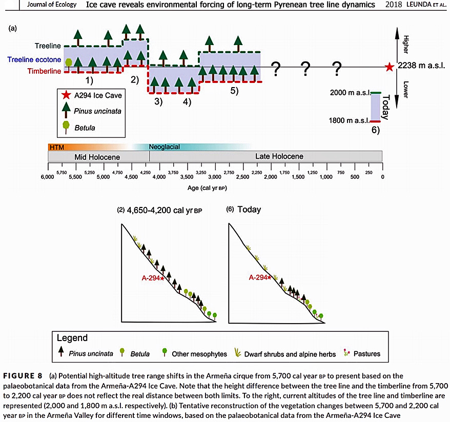
Leunda et al., 2018 (Spanish Pyrenees) The tree line ecotone was located at the cave altitude from 5,700 to 4,650 cal year bp, when vegetation consisted of open Pinus uncinata Ramond ex DC and Betula spp. Woodlands and timberline were very close to the site. Subsequently, tree line slightly raised and timberline reached the ice cave altitude, exceeding its today’s uppermost limit by c. 300–400 m during more than four centuries (4,650 and 4,200 cal year bp) at the end of the Holocene Thermal Maximum. After 4,200 cal year bp, alpine tundra communities dominated by Dryas octopetala L. expanded while tree line descended, most likely as a consequence of the Neoglacial cooling. Prehistoric livestock raising likely reinforced climate cooling impacts at 3,450– 3,250 cal year bp. Finally, a tree line ecotone developed around the cave that was on its turn replaced by alpine communities during the past 2,000 years. [Assuming a temperature lapse rate of +0.517°C/100 m {Navarro-Serrano et al., 2018}, a 300-400 m decline in today’s uppermost treeline limit would indicate that Pyrnees temperatures were about 1.81°C warmer than today during 4,650-4,200 cal year bp.]
A Warmer Past, Non-Hockey Stick Reconstructions
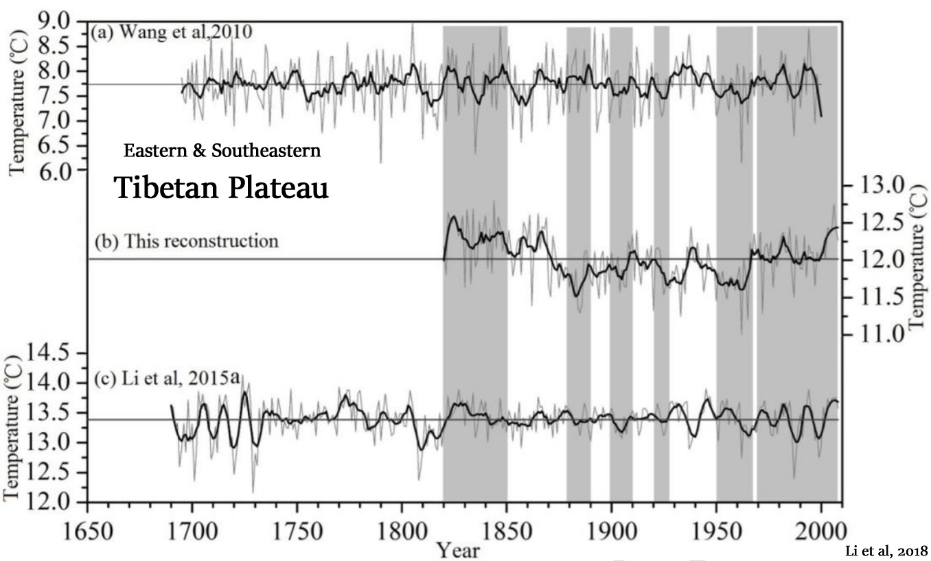
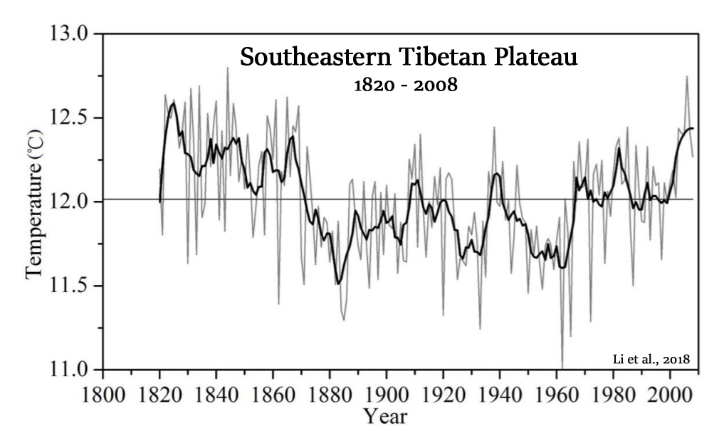
Li et al., 2018 There are also other studies that suggest that the recent climate warming over the southeastern TP actually began in the 1820s (Shi et al., 2015). However, a few reconstructions from the west and northwest parts of Sichuan or from the southeastern TP indicate that there were no obvious increase of temperature during the past decades (Li et al., 2015b; Zhu et al., 2016).
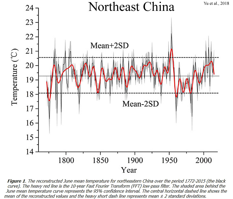
Yu et al., 2018 Reconstruction results explained 39.3% of climatic variance over the calibration period 1959–2015, and they indicated that the central XiaoXing Anling Mountains have experienced six major warm periods, five major cold periods, and several cold years that coincided with a sequence of major tropical volcanic eruptions. … Power spectrum revealed the existence of significant frequency cycles of variability at 2.0–2.3, 2.5–2.7, 2.9, 3.0, 3.4–4.5, 5.6, 7.2, 7.5–8.0, 8.2, 8.9, 9.9, 10.5–11.5, and 70.5 years, which may be linked to large-scale atmospheric-oceanic variability, such as the El Niño-Southern Oscillation, solar activity, and the Pacific Decadal Oscillation.
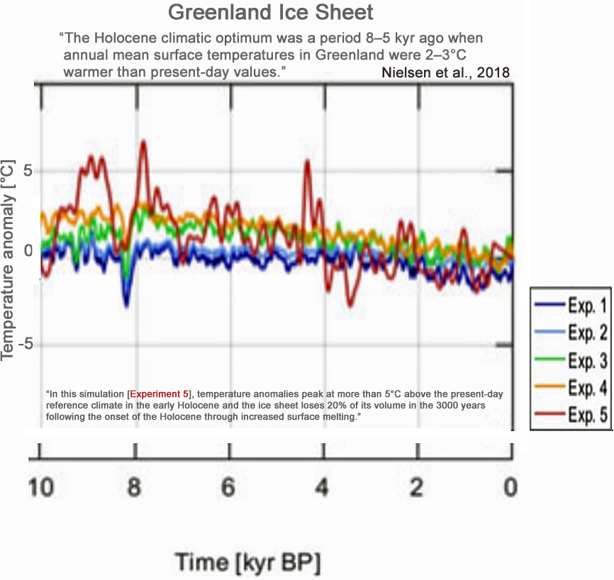
Nielsen et al., 2018 The Holocene climatic optimum was a period 8–5 kyr ago when annual mean surface temperatures in Greenland were 2–3°C warmer than present-day values. … We find that the ice sheet retreats to a minimum volume of ∼0.15–1.2 m sea-level equivalent smaller than present in the early or mid-Holocene when forcing an ice-sheet model with temperature reconstructions that contain a climatic optimum, and that the ice sheet has continued to recover from this minimum up to present day. … The initial mass loss in response to the temperature increase in the early Holocene is largest when forcing the ice sheet with the temperature and accumulation reconstructions from Gkinis and others (2014) (Experiment 5). In this simulation, temperature anomalies peak at more than 5°C above the present-day reference climate in the early Holocene and the ice sheet loses 20% of its volume in the 3000 years following the onset of the Holocene through increased surface melting. … The largest and most rapid retreat of the ice sheet was found for Experiment 5, which was forced by the temperature and accumulation reconstructions of Gkinis and others (2014). In this temperature reconstruction, temperature increases rapidly at the onset of the interglacial and has several shorter periods with temperatures more than 5°C above present in the early Holocene. .. Geological evidence suggests further that the ice-sheet margins in the southwest retreated up to ∼ 100km behind their present-day position during the mid-Holocene (Funder and others, 2011). This evidence is further supported by interpretations of relative sea-level records and bedrock uplift rates that also point towards ice sheet retreat beyond the present ice volume in the mid-Holocene (Khan and others, 2008; Funder and others, 2011; Lecavalier and others, 2014).
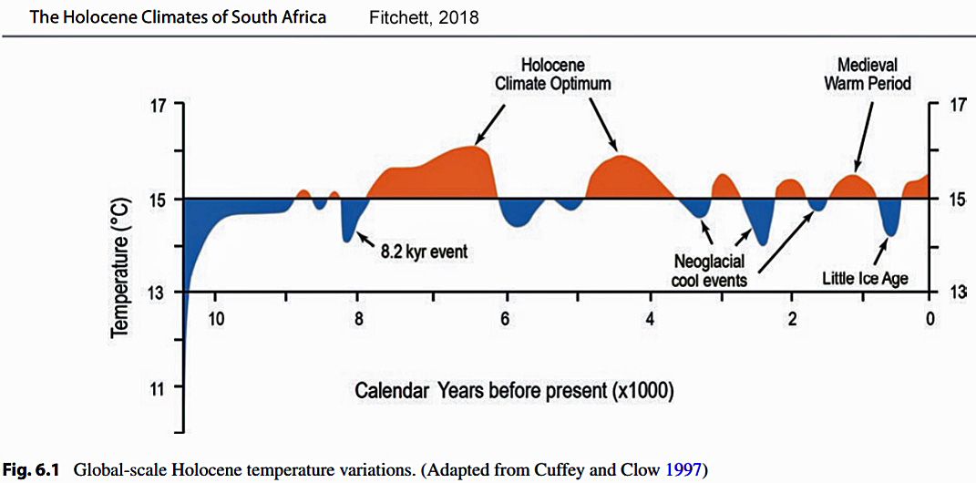
Fitchett, 2018 While the existence of a Little Ice Age cold event has been confirmed across much of the region, the local temperature decrease for this period remains to be quantitatively constrained. Suggestions of temperatures 1 °C colder than present during the Little Ice Age and 3 °C warmer than present in the earlier Medieval Warm Period (Tyson et al. 2000), remain unconfirmed against inferences of more severe cooling, as this event [Little Ice Age]reflects the most pronounced δ18O deviation within the 25,000 years.
Anderson et al., 2018 We estimate that air temperatures were 2.5–3.0 °C higher during the Holocene Thermal Maximum than the local 1960–1990 average. … Between 1700 and 1925 CE temperatures were likely 0.6–0.8 °C lower than the 1950–2015 reference temperature.
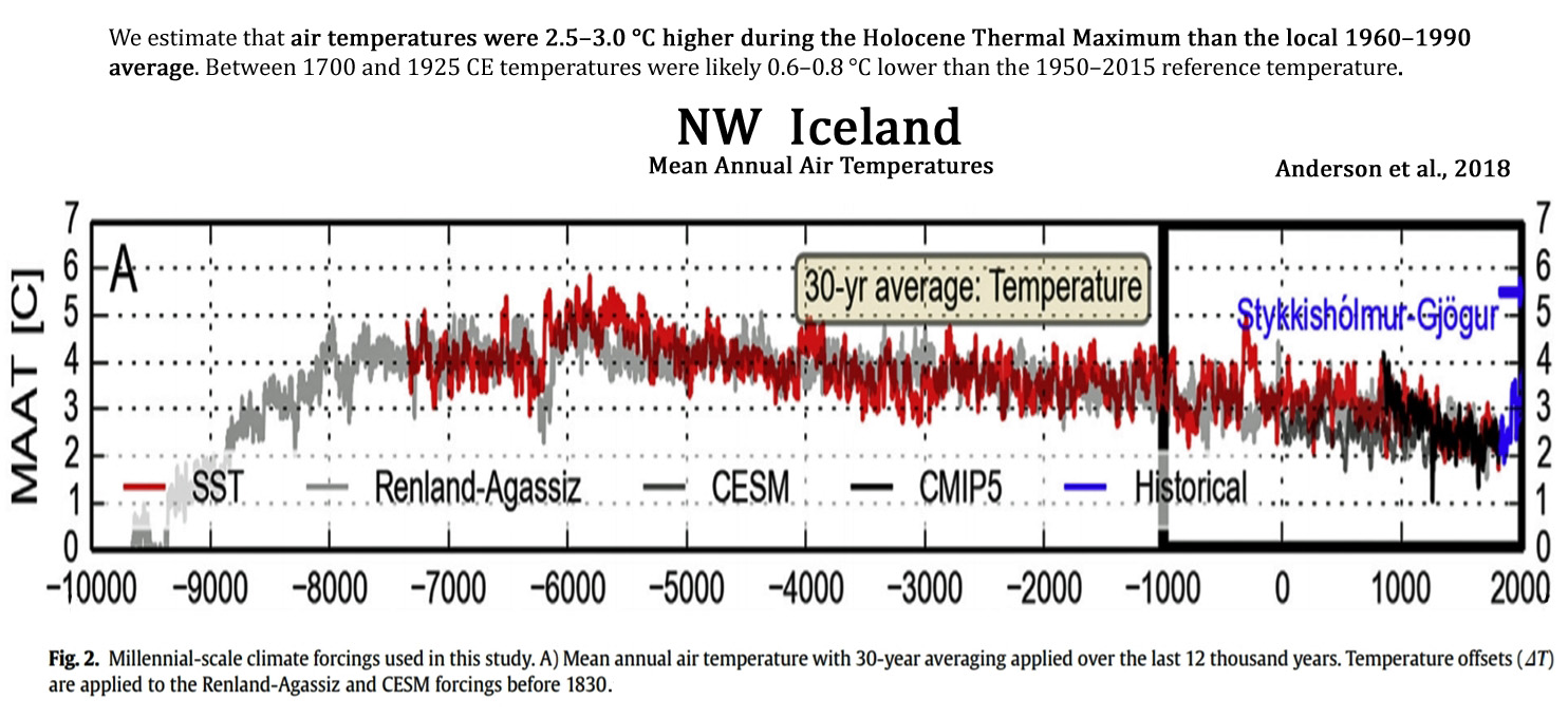
Harning et al., 2018 Iceland’s terrestrial HTM [Holocene Thermal Maximum] has previously been constrained to ~7.9 to 5.5 ka based on qualitative lake sediment proxies (Larsen et al., 2012; Geirsdottir et al., 2013), likely in association with progressive strengthening and warming of the Irminger Current (Castaneda et al., 2004; Smith et al., 2005; Olafsdottir et al., 2010). Numerical modeling experiments for Drangajokull suggest that peak air temperatures were 2.5 – 3°C warmer at this time relative to the 1961-1990 CE average (Anderson et al., 2018). … During the Little Ice Age (LIA, 1250-1850 CE), the Vestfirðir region entered the lowest multi centennial spring/summer temperature anomalies of the last 9 ka. Based on recent numerical modeling simulations, this anomaly is estimated to be 0.6-0.8°C below the 1950-2015 average on Vestfirðir (Anderson et al., 2018).
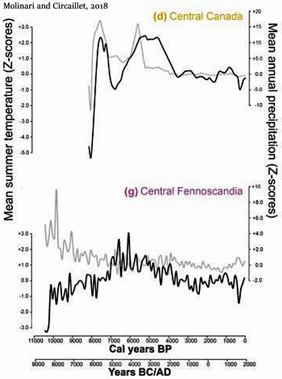
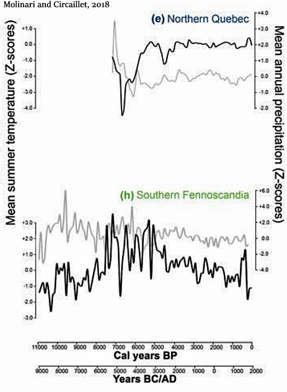
Molinari and Circaillet, 2018
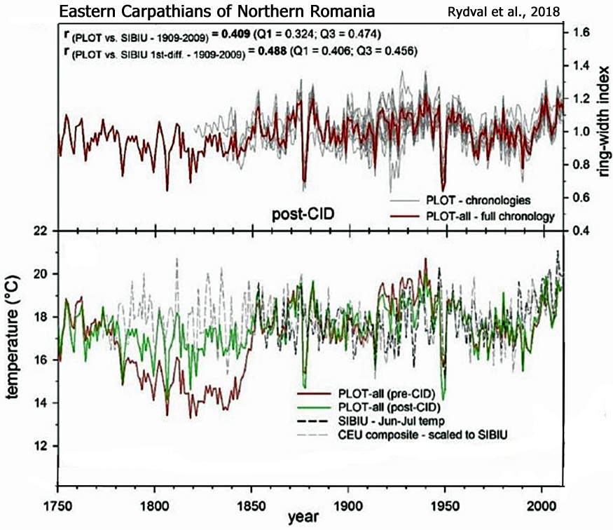
Rydval et al., 2018
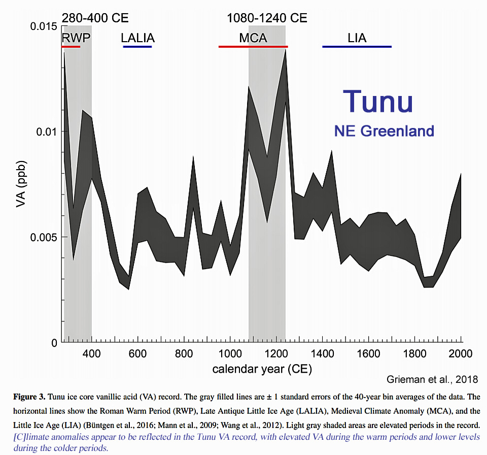
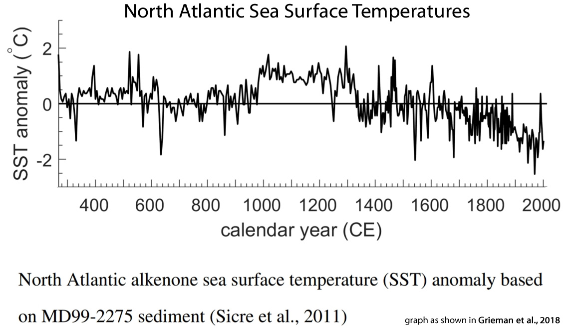
Grieman et al., 2018 [C]limate anomalies appear to be reflected in the Tunu VA [vanillic acid] record, with elevated VA [vanillic acid] during the warm periods and lower levels during the colder periods. The data suggest a positive correlation between North American fire and hemispheric mean temperature. This relationship could be due to climate-driven changes in temperature or precipitation on burning extent, frequency, or location, as well as to changes in atmospheric transport patterns. … … [E]levated VA [vanillic acid] early in the record [Roman Warm Period] and around the MCA [Medieval Climate Anomaly]. It also emphasizes the decreasing trend from 1200-1900 CE [Little Ice Age] and the increase during the 20th century [Current Warm Period].
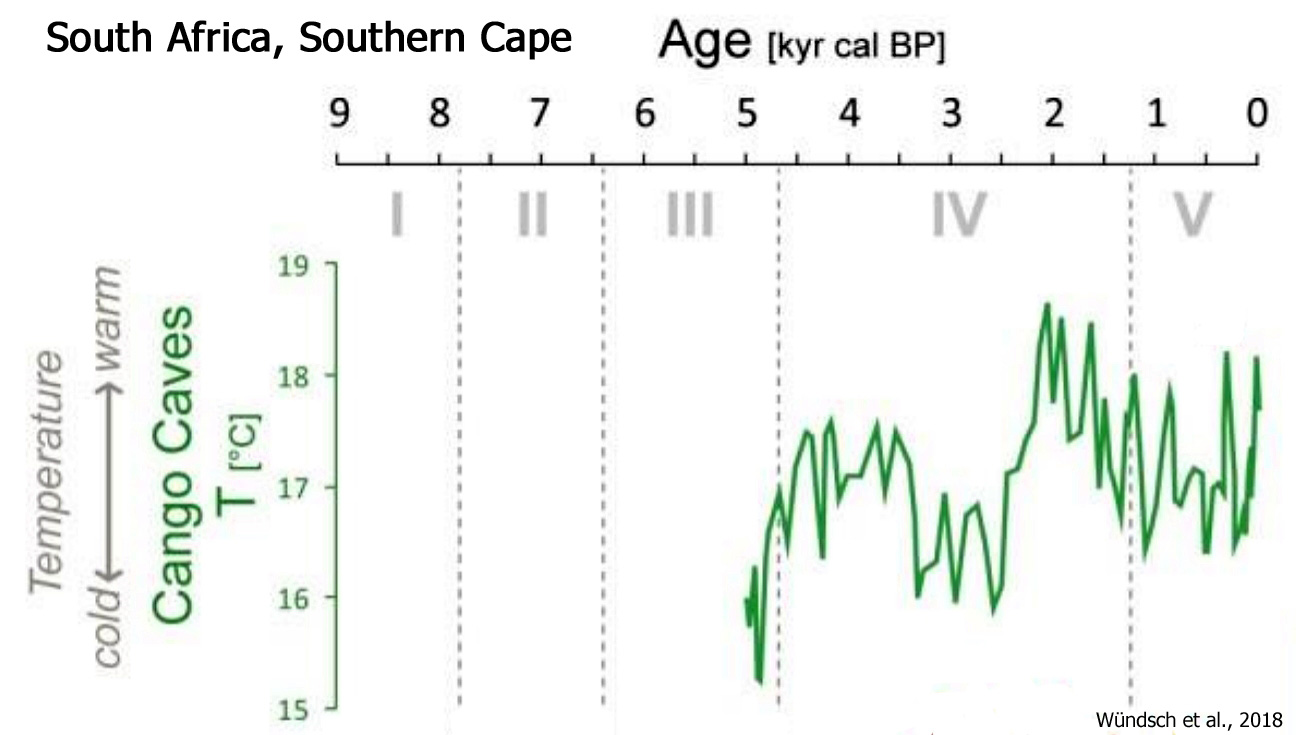
Wündsch et al., 2018
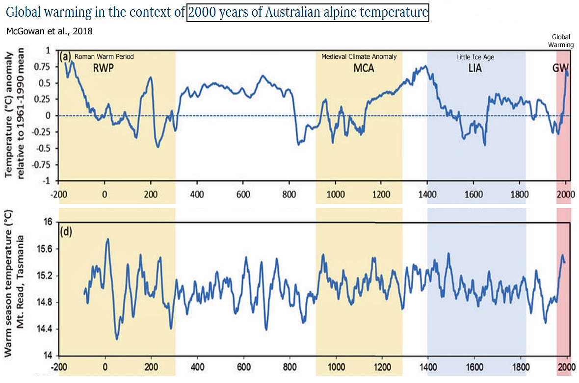
McGowan et al., 2018 Our reconstructed Tmax [temperature maximum] for these warmer conditions peaks around 1390 CE at + 0.8 °C above the 1961–90 mean, similar to the peak Tmax during the RWP [Roman Warm Period]. These results are aligned with the findings that show the period from 1150 to 1350 CE to be the warmest pre-industrial chronzone of the past 1000 yrs for southeast Australia.
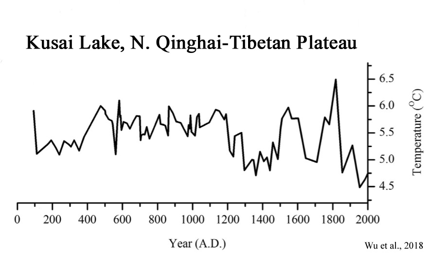
Wu et al., 2018
Bernabei et al., 2018
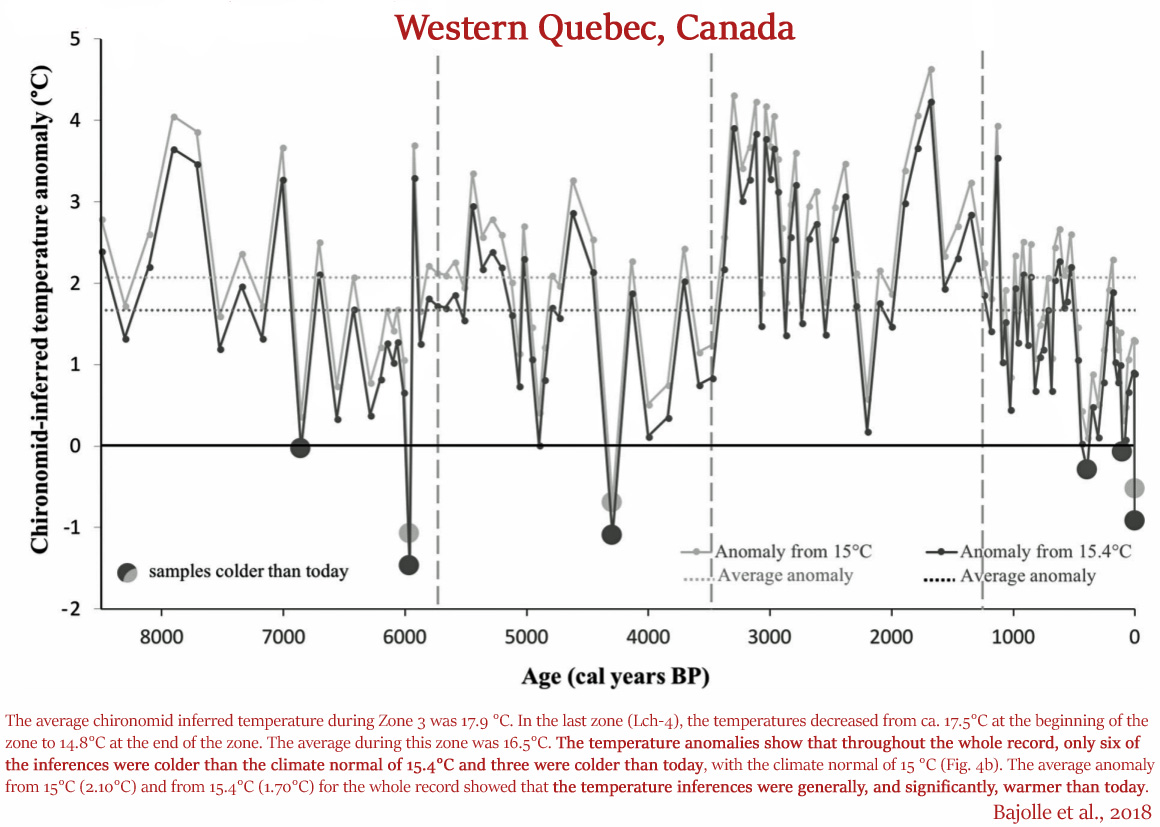
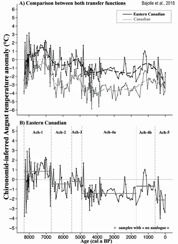
Bajolle et al., 2018 The mean annual temperature recorded at the closest meteorological station [La Sarre: 1961–1990] is 0.8 °C, with August temperature averages of 15.0 °C (1961–1990) and 15.4 °C (1981–2010). … During zone Lch1 (8500–5800 cal year BP), the average reconstructed temperature was 16.9 °C, with a decrease from 19 °C (maximum) to 17 °C at the end of the zone. In zone Lch-2 (ca. 5700–3500 cal year BP), temperatures had an average of 16.8 °C, with a decrease from 17.8 °C around 5200 cal year BP to 16.2 °C at 3400 cal year BP. Zone Lch-3 (ca. 3500–1200 cal year BP) started with inferences for high temperatures (19.3–18.5 °C), followed by a decrease to 16.8 °C between ca. 3000 and 2500 cal year BP. An increase (18.3 and 19.6 °C) was inferred for the period between 1800 and 1500 cal year BP. The average chironomid inferred temperature during Zone 3 was 17.9 °C. In the last zone (Lch-4), the temperatures decreased from ca. 17.5 °C at the beginning of the zone to 14.8 °C at the end of the zone. The average during this zone was 16.5 °C. The temperature anomalies show that throughout the whole record, only six of the inferences were colder than the climate normal of 15.4 °C and three were colder than today, with the climate normal of 15 °C (Fig. 4b). The average anomaly from 15 °C (2.10 °C) and from 15.4 °C (1.70 °C) for the whole record showed that the temperature inferences were generally, and significantly, warmer than today.
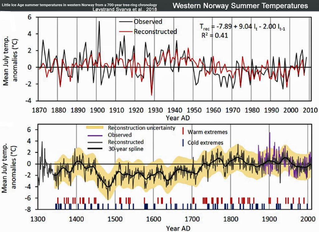
Løvstrand Svarva 2018 et al., 2018 A ring-width Pinus sylvestris chronology from Sogndal in western Norway was created, covering the period AD 1240–2008 and allowing for reconstruction of monthly mean July temperatures. This reconstruction is the first of its kind from western Norway and it aims to densify the existing network of temperature-sensitive tree-ring proxy series to better understand past temperature variability in the ‘Little Ice Age’ and diminish the spatial uncertainty. Spatial correlation reveals strong agreement with temperatures in southern Norway, especially on the western side of the Scandinavian Mountains. Five prominent cold periods are identified on a decadal timescale, centred on 1480, 1580, 1635, 1709 and 1784 and ‘Little Ice Age’ cooling spanning from 1450 to the early 18th century. High interannual and decadal agreement is found with an independent temperature reconstruction from western Norway, which is based on data from grain harvests and terminal moraines.
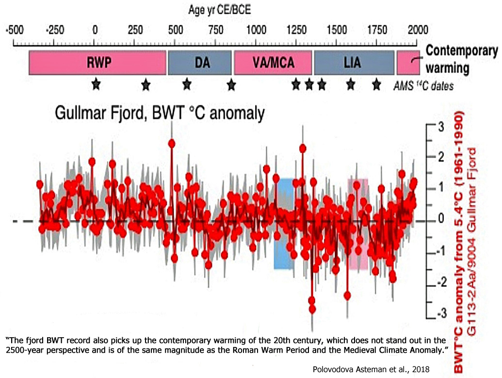
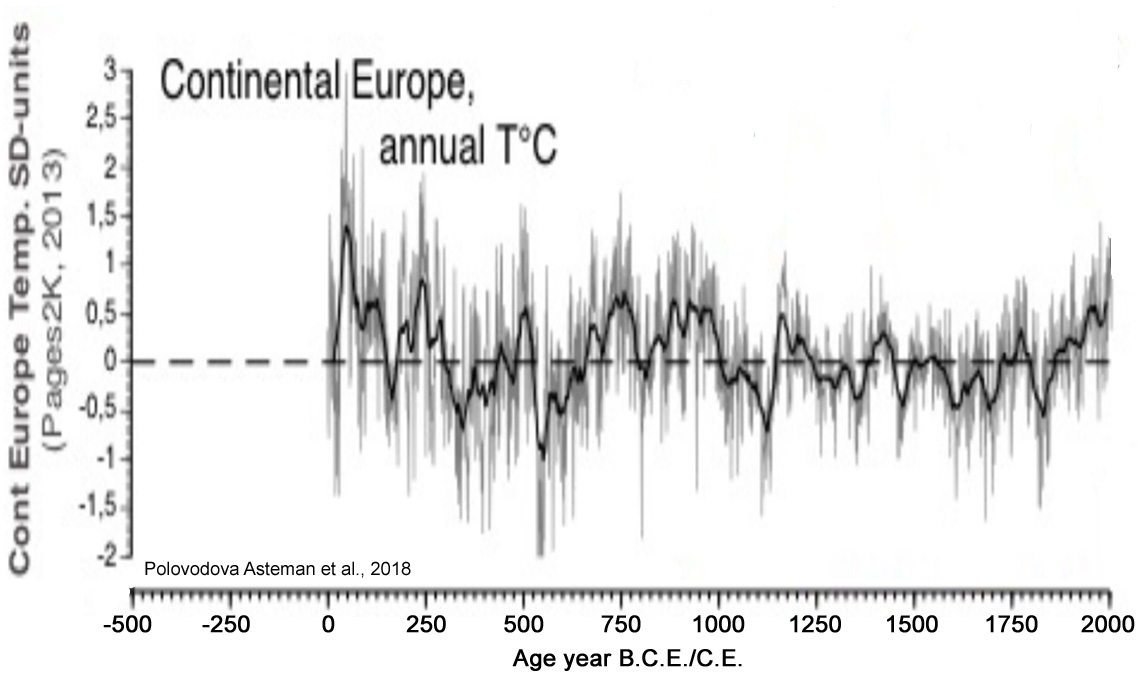
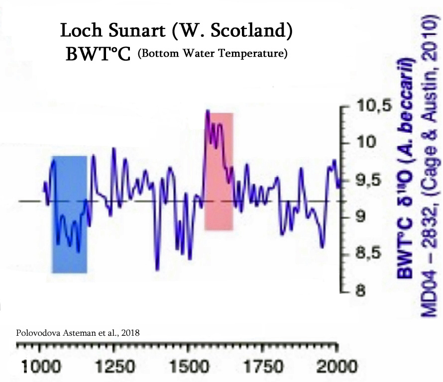
Polovodova Asteman et al., 2018 The record demonstrates a warming during the Roman Warm Period (~350 BCE – 450 CE), variable bottom water temperatures during the Dark Ages (~450 – 850 CE), positive bottom water temperature anomalies during the Viking Age/Medieval Climate Anomaly (~850 – 1350 CE) and a long-term cooling with distinct multidecadal variability during the Little Ice Age (~1350 – 1850 CE). The fjord BWT [bottom water temperatures, Western Sweden] record also picks up the contemporary warming of the 20th century, which does not stand out in the 2500-year perspective and is of the same magnitude as the Roman Warm Period and the Medieval Climate Anomaly.
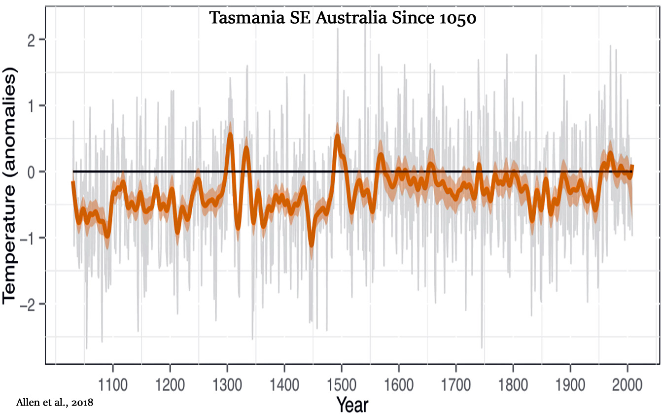
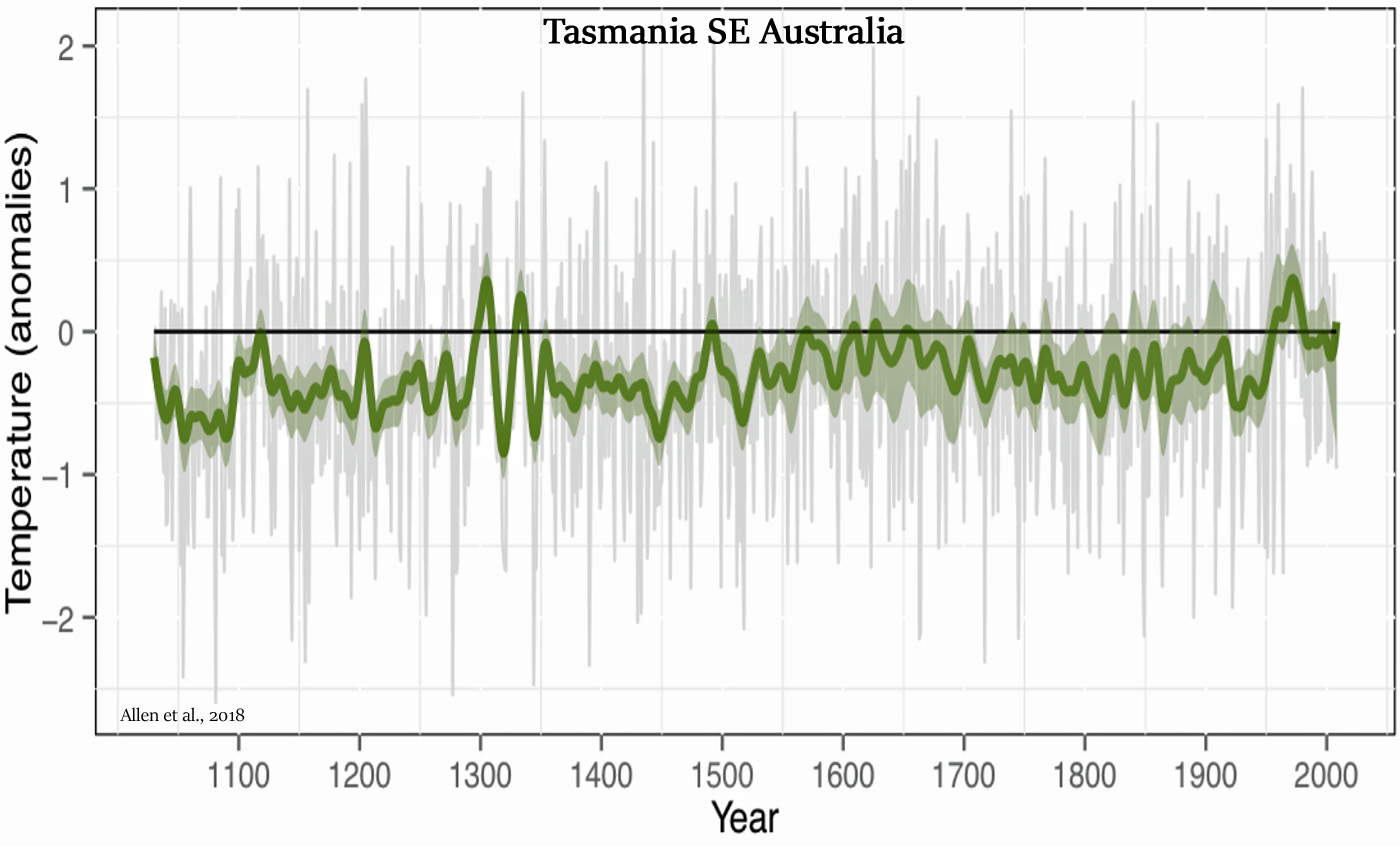
Allen et al., 2018 The longest sustained period of relatively high temperatures in the reconstructions is the post 1950 CE period although there are clearly individual years much earlier that were warmer than any in the post-1950 period.
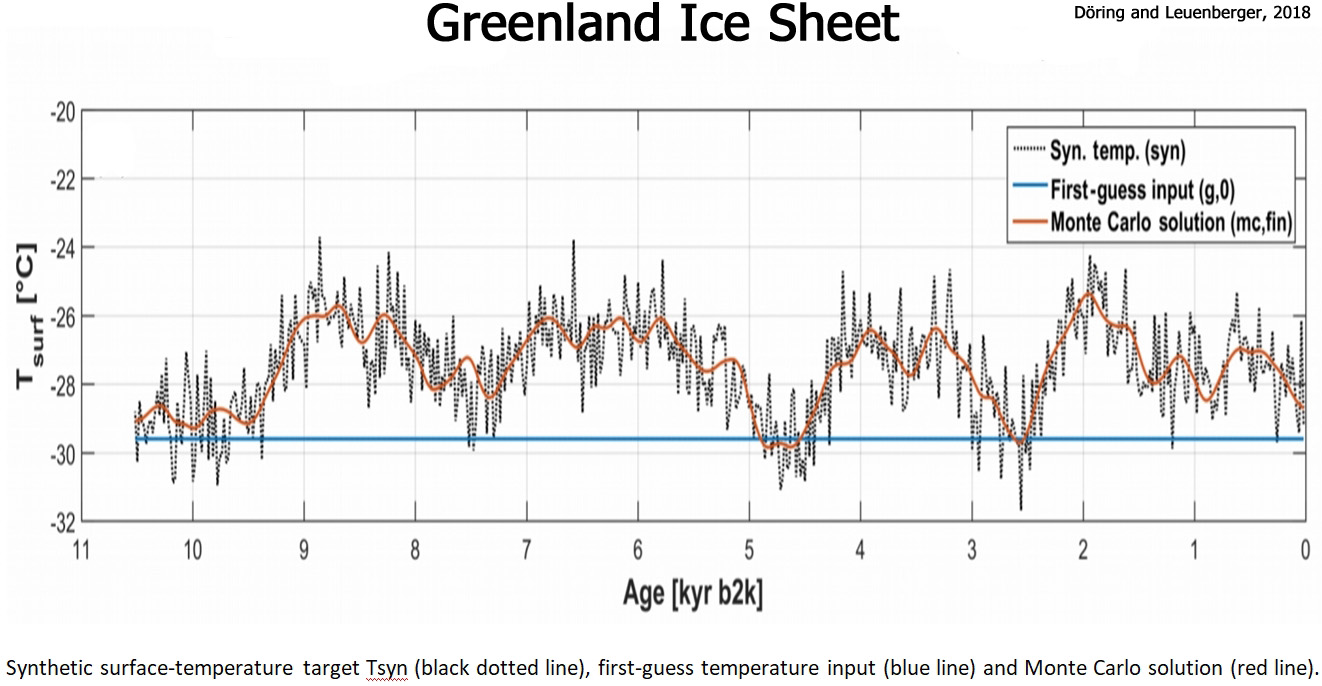
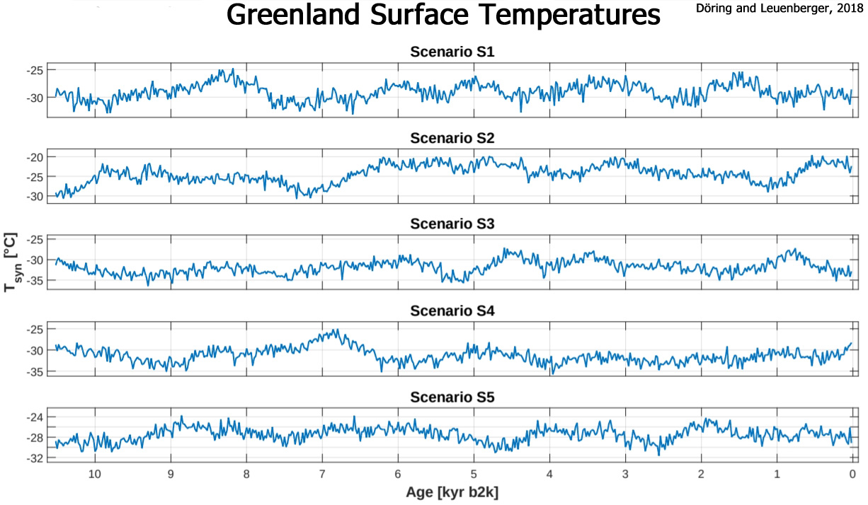
Döring and Leuenberger, 2018
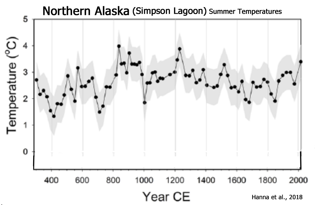
Hanna et al., 2018 Here, we utilize one such sediment archive from Simpson Lagoon, Alaska, located adjacent to the Colville River Delta to reconstruct temperature variability and fluctuations in sediment sourcing over the past 1700 years. Quantitative reconstructions of summer air temperature […] reveal temperature departures correlative with noted climate events (i.e. ‘Little Ice Age’, ‘Medieval Climate Anomaly’). … Reconstructed temperatures are generally coolest between 300 and 800 CE (Tavg = 2.24 ± 0.98°C), displaying three temperature minima centered at 410 CE (1.34 ± 0.72°C), 545 CE (1.91 ± 0.69°C), and 705 CE (1.49 ± 0.69°C). Temperatures then rapidly increased, reaching the warmest interval (800–1000 CE) in the approximately 1700-year record. During this interval, average temperatures were 3.31 ± 0.65°C, with a maximum temperature of 3.98°C.
Miller et al., 2018
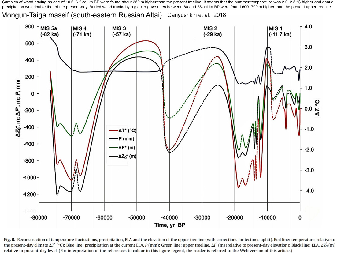
Ganyushkin et al., 2018 (full paper) Samples of wood having an age of 10.6–6.2 cal ka BP were found about 350 m higher than the present treeline. It seems that the summer temperature was 2.0–2.5 °C higher and annual precipitation was double that of the present-day. … Buried wood trunks by a glacier gave ages between 60 and 28 cal ka BP and were found 600–700 m higher than the present upper treeline. This evidences a distinctly elevated treeline during MIS 3a and c. With a correction for tectonics we reconstructed the summer warming to have been between 2.1 and 3.0 °C [higher than today].
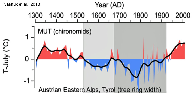
Ilyashuk et al., 2018 Here we present a high-resolution (4–10 years) 700-year long mean July air temperature reconstruction based on subfossil chironomid assemblages from a remote lake in the Austrian Eastern Alps to gain further insights into the LIA climatic deterioration in the region. The record provides evidence for a prolonged period of predominantly cooler conditions during AD 1530–1920, broadly equivalent to the climatically defined LIA in Europe. The main LIA phase appears to have consisted of two cold time intervals divided by slightly warmer episodes in the second half of the 1600s. The most severe cooling occurred during the eighteenth century. The LIA temperature minimum about 1.5 °C below the long-term mean recorded in the mid-1780 s coincides with the strongest volcanic signal found in the Greenland ice cores over the past 700 years and may be, at least in part, a manifestation of cooling that followed the long-lasting AD 1783–1784 Laki eruption. A continuous warming trend is evident since ca AD 1890 (1.1 °C in 120 years). The chironomid-inferred temperatures show a clear correlation with the instrumental data and reveal a close agreement with paleotemperature evidence from regional high-elevation tree-ring chronologies. A considerable amount of the variability in the temperature record may be linked to changes in the North Atlantic Oscillation.
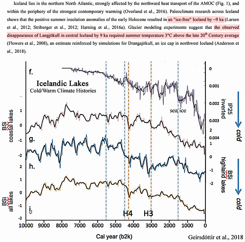
Geirsdóttir et al., 2018 Paleoclimate research across Iceland shows that the positive summer insolation anomalies of the early Holocene resulted in an “ice-free” Iceland by ~9 ka (Larsen et al., 2012; Striberger et al., 2012; Harning et al., 2016a). Glacier modeling experiments suggest that the observed disappearance of Langjökull in central Iceland by 9 ka required summer temperature 3°C above the late 20th Century average (Flowers et al., 2008), an estimate reinforced by simulations for Drangajökull, an ice cap in northwest Iceland (Anderson et al., 2018).
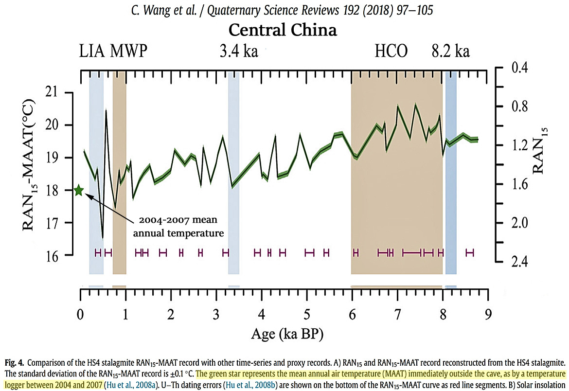
Wang et al., 2018 The average RAN15-MAAT of 18.4°C over the most recent part of the record (<0.8 ka BP) [the last 800 years BP] overlaps with the range of MAATs, ca. 16.2°C to 18.7°C (av. 17.5°C) measured since 1952 at the nearest meteorological station (Yichang, located ca. 100 km away) and is very close to the av. MAAT of 18°C measured directly outside the cave by a temperature logger between 2004 and 2007 (Hu et al., 2008a). This agreement between reconstructed temperatures and instrumental measurements increases our confidence in the potential of the RAN15 proxy. RAN15-MAATs in HS4 vary from 16.5°C to 20.6°C (av. 19°C), during the last 9 ka BP, and broadly follow a long-term trend of declining temperatures in line with declining solar insolation at 30°N in July (Laskar et al., 2004) (Fig. 4B). The temperature variation (4.1°C) in our record is larger than the calibration error of the RAN15 proxy (RMSE ¼ 2.6°C; Wang et al., 2016). … The Holocene Climate Optimum (HCO) shown in the RAN15-MAAT record is from 8 to 6 ka BP, with the highest temperature at ca. 7.0 ka BP. Superimposed on the orbital-scale Holocene trend are centennial to millennial scale climate fluctuations of ca. 1-2°C. Interestingly, the most recent 0.9 ka BP [900 years BP] is distinguished by greater variability with the highest (20.5°C) and lowest (16.5°C) RAN15-MAATs occurring consecutively at 0.6 ka BP [600 years BP] and 0.5 ka BP [500 years BP]. [Surface temperatures dropped by -4.0°C within ~100 years.]
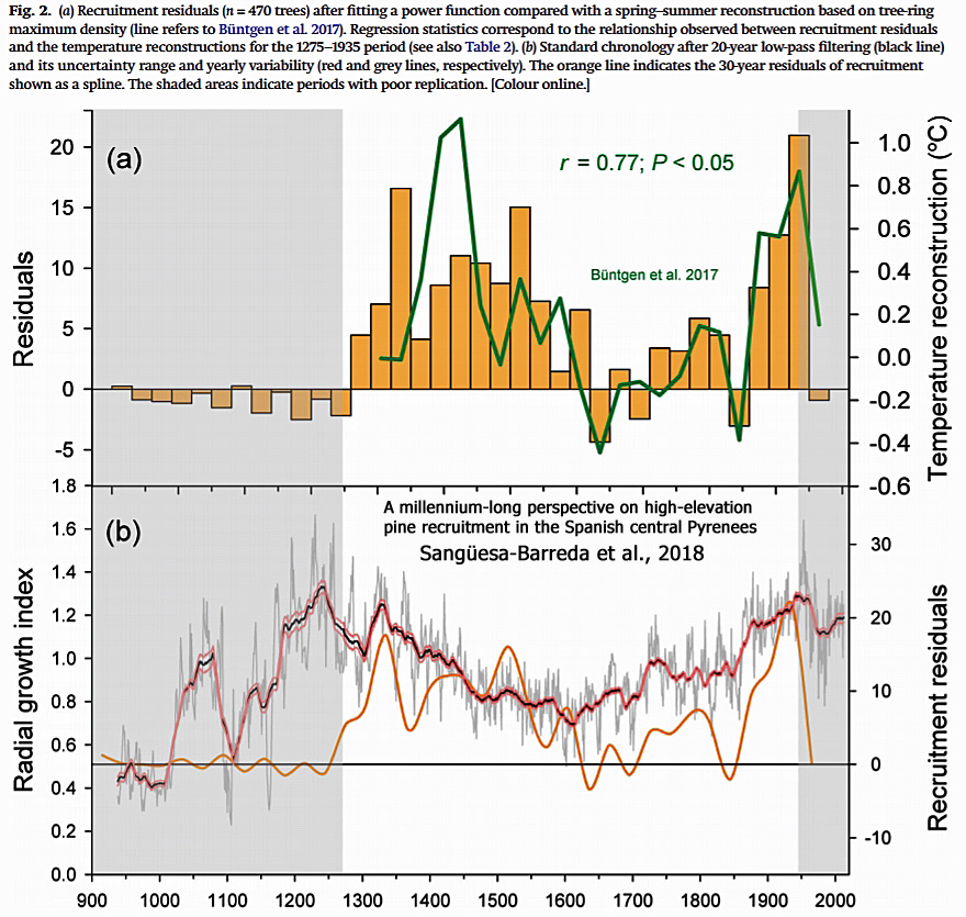
Sangüesa-Barreda et al., 2018 In summary, we found that tree recruitment in a tree-line ecotone in the Spanish central Pyrenees was enhanced during warm periods, whereas cold periods were associated with relatively low recruitment rates. Tree-ring records reveal that temperature is the major driver of long-term tree population dynamics in cold-limited environments.
Wang et al., 2018 The average RAN15-MAAT of 18.4°C over the most recent part of the record (<0.8 ka BP) [the last 800 years BP] overlaps with the range of MAATs, ca. 16.2°C to 18.7°C (av. 17.5°C) measured since 1952 at the nearest meteorological station (Yichang, located ca. 100 km away) and is very close to the av. MAAT of 18°C measured directly outside the cave by a temperature logger between 2004 and 2007 (Hu et al., 2008a). This agreement between reconstructed temperatures and instrumental measurements increases our confidence in the potential of the RAN15 proxy. RAN15-MAATs in HS4 vary from 16.5°C to 20.6°C (av. 19°C), during the last 9 ka BP, and broadly follow a long-term trend of declining temperatures in line with declining solar insolation at 30°N in July (Laskar et al., 2004). … Interestingly, the most recent 0.9 ka BP [900 years BP] is distinguished by greater variability with the highest (20.5°C) and lowest (16.5°C) RAN15-MAATs occurring consecutively at 0.6 ka BP [600 years BP] and 0.5 ka BP [500 years BP]. [Surface temperatures dropped by -4.0°C within ~100 years.]
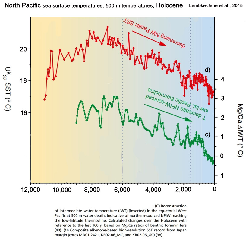
Lembke-Jene et al., 2018 Importantly, recent low-latitude mid-depth thermocline temperature changes (at around 500 m water depth) in the equatorial West Pacific show concomitant higher temperatures in the EMH [Early to Mid Holocene, 11 to 6 thousand years ago] of similar magnitude, with northern NPIW-sourced thermocline or intermediate water temperatures (Fig. 3C) being warmer by 2.1 ± 0.4 °C than during the last century [Rosenthal et al., 2013], in strong accord with our assumed decrease in ventilation in OSIW and NPIW.
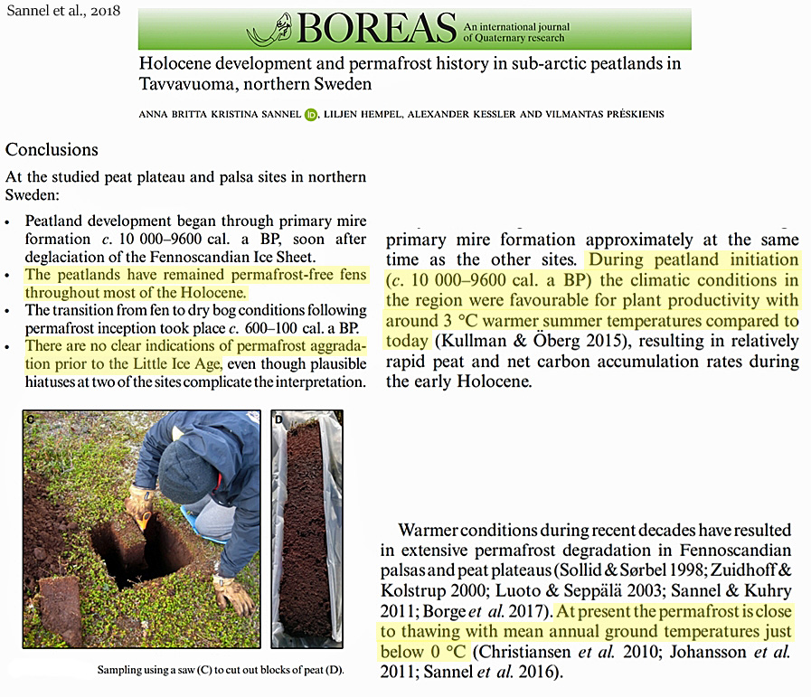
Sannel et al., 2018 (Subarctic Northern Sweden) At all these sites the datings together with the results of the plant macrofossil analyses suggest that permafrost aggradation took place around 600–100 cal. a BP [the Little Ice Age]. … [A]t these sites there are no indications of permafrost inception prior to the Little Ice Age. … Warmer conditions during recent decades have resulted in extensive permafrost degradation in Fennoscandian palsas and peat plateaus (Sollid& Sørbel 1998; Zuidhoff& Kolstrup 2000; Luoto & Seppala 2003; Sannel & Kuhry 2011; Borge et al. 2017). At present the permafrost is close to thawing with mean annual ground temperatures just below 0 °C (Christiansen et al. 2010; Johansson et al. 2011; Sannel et al. 2016). … Throughout most of the Holocene, these northern peatlands have not experienced climatic conditions cold enough for permafrost to form. … During peatland initiation (c. 10 000–9600 cal. a BP) the climatic conditions in the region were favourable for plant productivity with around 3 °C warmer summer temperatures compared to today (Kullman & Oberg 2015), resulting in relatively rapid peat and net carbon accumulation rates during the early Holocene. [Subarctic Northern Sweden has yet to fully recover from the Little Ice Age cooling, as permafrost still exists in regions where there was no recorded permafrost during nearly all of the last 10,000 years.]
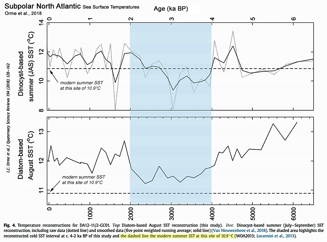
Orme et al., 2018 The diatom-based reconstruction shows warmer reconstructed temperatures than the dinocyst-based reconstruction and the modern measured summer SST (June-August) of 10.9°C. … The overall long-term cooling trend in the diatom-based SST reconstruction for the last 6.1 ka fits with the widely established cooling in the subpolar North Atlantic since the Holocene Thermal Maximum, resulting from decreasing Northern Hemisphere summer insolation (e.g. Calvo et al., 2002; Marchal et al., 2002; Andersen et al., 2004a, 2004b; Andersson et al., 2010; Jiang et al., 2015; Sejrup et al., 2016). … The earliest warm period at ~6.1-4 ka BP had average reconstructed SSTs of 12-13.3°C, with the warmest temperatures in the record occurring at ~6.1-5.5 ka BP (c. 13°C). The cooler period ~4-2 ka BP had reconstructed SST that varied around 11.5°C, with minima at 3.2 and 2.4 ka BP interrupted by a short warming at 2.7 ka BP. In the most recent period after 2 ka BP the SSTs again increased peaking at 1.8 ka BP, yet SSTs did not attain values as high as those reconstructed for 6.1-4 ka BP. … In the diatom-based record the mean reconstructed temperature between 4 and 2 ka BP is 11.5°C compared with 12.5 and 12.1°C in the periods before 4 ka BP and after 2 ka BP respectively, showing a reconstructed cooling of 0.6-1°C. In the dinocyst-based record the mean reconstructed temperature between 4 and 2 ka BP is 10.3°C compared with 11.3 and 11.6°C in the periods before 4 ka BP and after 2 ka BP respectively, showing a cooling of 1-1.3°C.
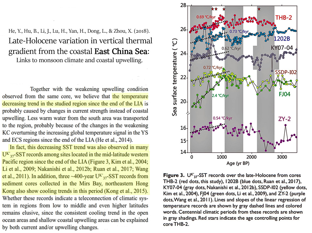
He et al., 2018 Together with the weakening upwelling condition observed from the same core, we believe that the temperature decreasing trend in the studied region since the end of the LIA [(the recent ~100 years)] is probably caused by changes in current strength instead of coastal upwelling. Less warm water from the south area was transported to the region, probably because of the changes in the weakening KC overturning the increasing global temperature signal in the YS and ECS regions since the end of the LIA (He et al., 2014). In fact, this decreasing SST trend was also observed in many UK’37-SST records among sites located in the mid-latitude western Pacific region since the end of the LIA (Figure 3, Kim et al., 2004; Li et al., 2009; Nakanishi et al., 2012b; Ruan et al., 2017; Wang et al., 2011). In addition, three ~400-year UK’37-SST records from sediment cores collected in the Mirs Bay, northeastern Hong Kong also show cooling trends in this period (Kong et al., 2015).
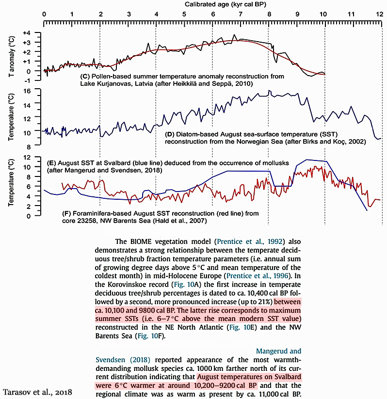
Tarasov et al., 2018 In the Korovinskoe record (Fig. 10A) the first increase in temperate deciduous tree/shrub percentages is dated to ca. 10,400 cal BP followed by a second, more pronounced increase (up to 21%) between ca. 10,100 and 9800 cal BP. The latter rise corresponds to maximum summer SSTs (i.e. 6-7°C above the mean modern SST value) reconstructed in the NE North Atlantic (Fig. 10E) and the NW Barents Sea (Fig. 10F). … A pollen-based reconstruction of the summer temperature anomaly at Lake Kurjanovas (Fig. 1) in Latvia suggests that the warmest interval in the area located ca. 270 km west of Korovinskoe occurred ca. 8100-5600 cal BP (Fig. 10C; Heikkila and Seppa, 2010). … Mangerud and Svendsen (2018) reported appearance of the most warmth-demanding mollusk species ca. 1000 km farther north of its current distribution indicating that August temperatures on Svalbard were 6°C warmer at around 10,200-9200 cal BP and that the regional climate was as warm as present by ca. 11,000 cal BP.
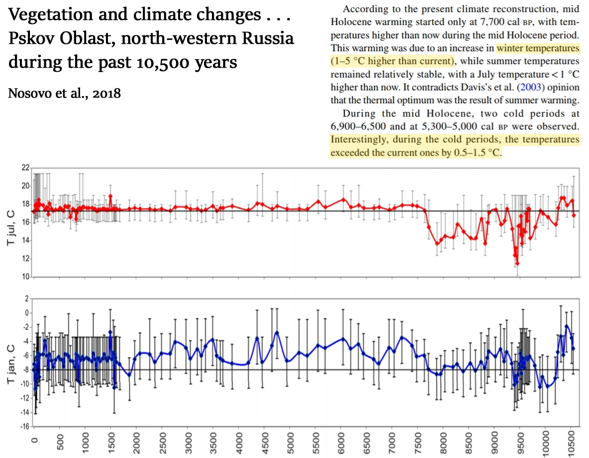
Nosova et al., 2018 According to the present climate reconstruction, mid Holocene warming started only at 7,700 cal bp, with temperatures higher than now during the mid Holocene period. This warming was due to an increase in winter temperatures (1–5 °С higher than current), while summer temperatures remained relatively stable, with a July temperature<1 °С higher than now. … During the mid Holocene, two cold periods at 6,900–6,500 and at 5,300–5,000 cal bp were observed. Interestingly, during the cold periods, the temperatures exceeded the current ones by 0.5–1.5 °С. … The transition from the mid Holocene thermal maximum to the following period occurred without considerable climatic changes. The mean annual temperatures remained much higher than the current ones by 0.5–2.5 °С until 2,500 cal bp. Local maximum temperatures were observed at 4,800, 4,300, 3,500 and 2,900–2,700 cal bp. The present climatic reconstruction demonstrates a gradual cooling down to current levels at ca. 2,500 cal bp, and then followed by a new warming phase with up to 1–2 °С increase at approximately 1,500 cal bp.
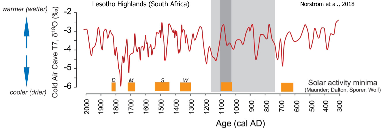
Norström et al., 2018 The first part of the multi-proxy record (AD 400–800) shows stable terrestrial conditions and low detrital input, followed by higher variability in almost all proxies between ca. AD 900 and 1200. The δ13 C record infers a higher proportion of C4 vegetation, tentatively associated with higher temperatures during this phase, coeval with the Medieval Climate Anomaly (MCA). … Although age-model constraints impedes a robust regional comparison, the inferred climate variability is discussed as a tentative response to enhanced mid-latitude cyclonic activity during LIA, and the variable MCA climate conditions as indirectly dictated by changes in solar activity.
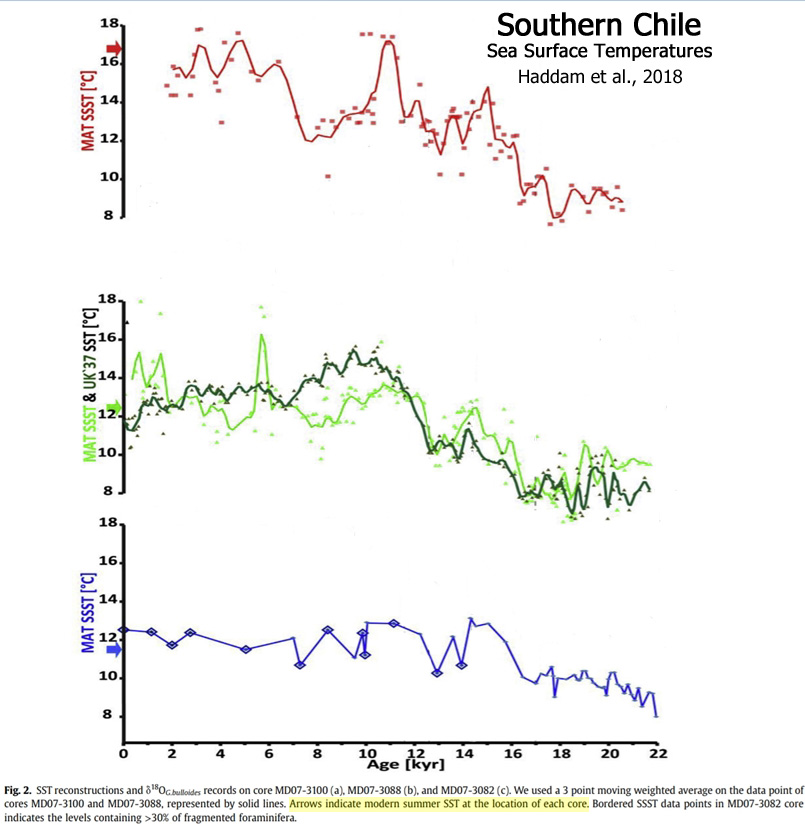
Haddam et al., 2018 The MD07-3100 SSST [summer sea surface temperature] reconstruction displays values ranging from 8° to 17°C over the last 21 kyr. Lowest temperatures are recorded at 18 kyr just before the onset of the deglaciation, while the warmest ones are recorded at 15 kyr (15-17°C), from 11 to 10 kyr and from 4.7 to 3 kyr. After 6.5 kyr, SSSTs stay mostly 15°C and are marked by two short-term warming events up to ~18°C, at 4.7 and 3.1 kyr respectively until reaching the present-day summer temperature values at the core location. … Core MD07-3088 displays SSST values ranging from 7 to 18°C over the last 21.4 kyr. The lowest values are observed from 18.3 to 16.5 kyr, while the highest are recorded during the middle to late Holocene (at 5.7, 1.5 and 0.7 kyr respectively). The Early Holocene, from 11.5 kyr to 10 kyr, is characterized by SSST values at around 13°C followed by a progressive 1.5°C decreasing trend until 7.7 kyr. Then a sharp SSST increase culminated at 5.8 kyr (~16°C) before decreasing again at 4.5 kyr. … The UK 37 SST reconstructions for core MD07-3088 show similar trends compared to MAT-SSST displaying the lowest and highly variable temperatures between 21 and 18 kyr. [A] sharp SST increase (~5°C) marks the Early Holocene (~10.4 kyr). Between 10.4 and 6.5 kyr, SST decreased again, followed by a plateau until 3 kyr with mean values of 13°C. Finally, after an abrupt SST rise (~2°C) centered at 1.5 kyr, UK 37 SST decrease until present-day. … The MAT SSST reconstruction of core MD07-3082 shows values ranging from 9°C to 13°C over the last 22 kyr. The lowest temperatures are recorded between 22 and 20.5 kyr, whereas a progressive SSST increase representing the last deglaciation culminates at 14.3 kyr. A two-step SSST lowering of about 3°C is recorded between 14.3 and 12.9 kyr and attributed to the ACR before reaching stable values at 12°C during the Holocene.
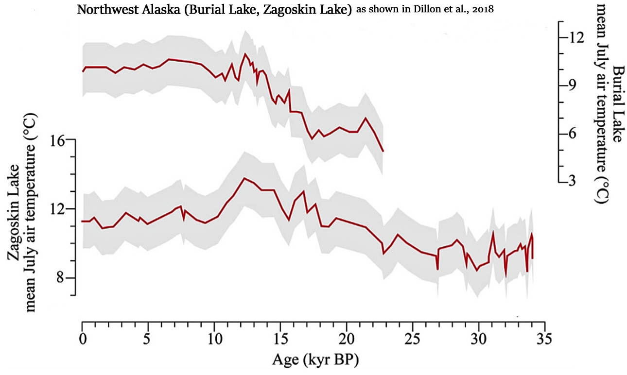
Dillon et al., 2018
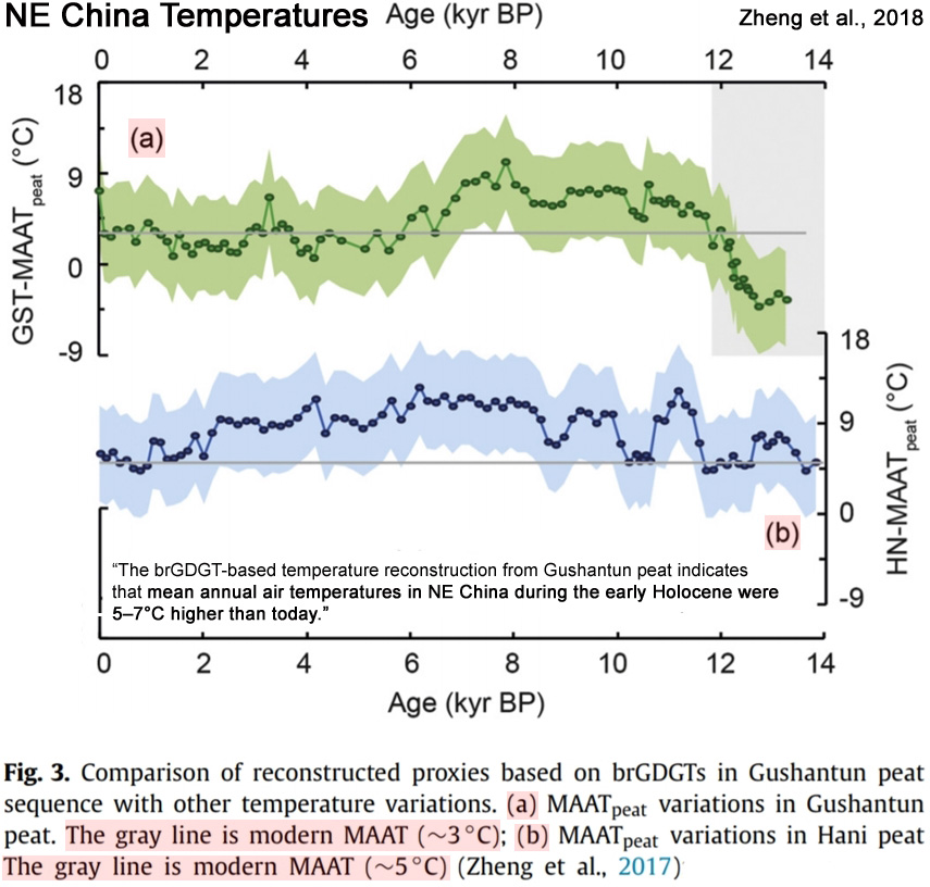
Zheng et al., 2018 In this study we present a detailed GDGT data set covering the last 13,000 years from a peat sequence in the Changbai Mountain in NE China. The brGDGT-based temperature reconstruction from Gushantun peat indicates that mean annual air temperatures in NE China during the early Holocene were 5–7°C higher than today. Furthermore, MAAT records from the Chinese Loess Plateau also suggested temperature maxima 7–9°C higher than modern during the early Holocene (Peterse et al., 2014; Gao et al., 2012; Jia et al., 2013). Consequently, we consider the temperatures obtained using the global peat calibration to be representative of climate in (NE) China. … The highest temperatures occurred between ca. 8 and 6.8 kyr BP, with occasional annual mean temperatures >8.0 ± 4.7°C, compared to the modern-day MAAT of ∼3°C.
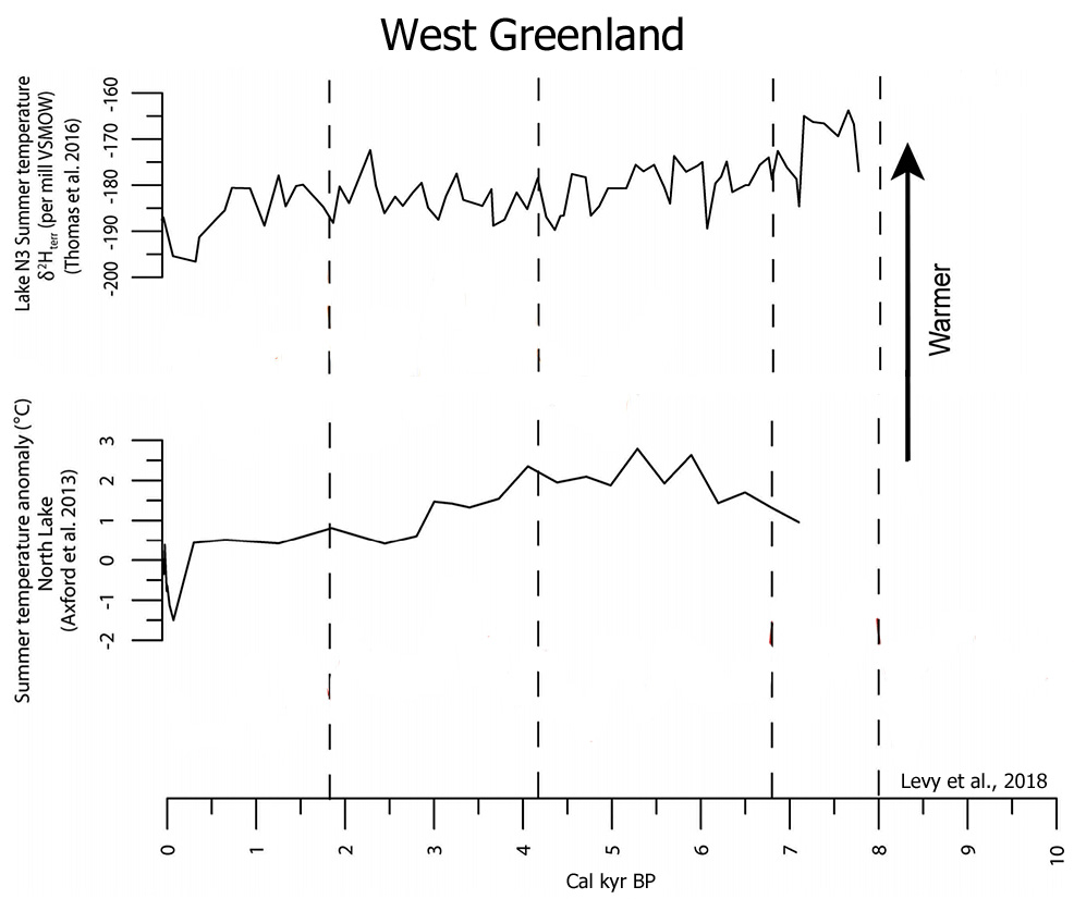
Levy et al., 2018 The three historical moraine crests indicate that there were at least three ice-margin stillstands or advances during historical time. Summer temperature records from North lake (Axford et al. 2013) and Lake N3 (Thomas et al. 2016) broadly register cooling in the past 200 years in western Greenland, which likely influenced the advance to the historical moraines.
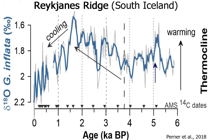
Perner et al., 2018 From c. 1.5 ka BP onwards, we record a prominent subsurface cooling and continued occurrence of fresh and sea‐ice loaded surface waters at the study site.
Belle et al., 2018
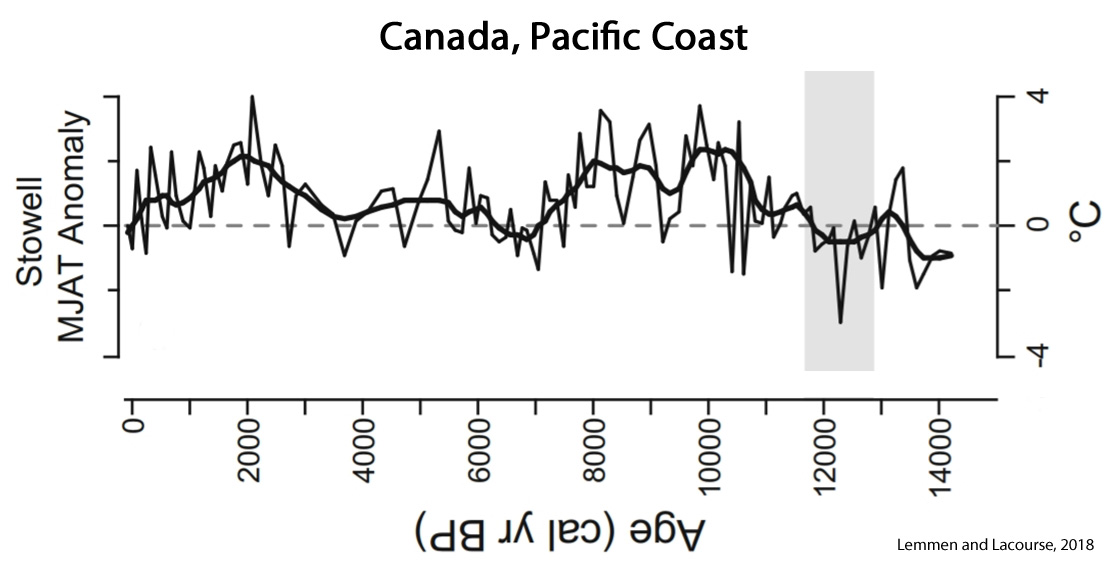
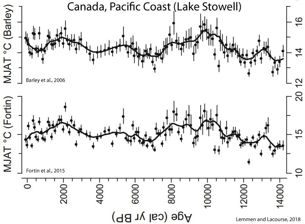
Lemmen and Lacourse, 2018 The early Holocene was marked by relatively stable temperatures that exceeded modern by ~2 to 3°C. Inferred temperatures generally decrease through the remainder of the Holocene.

Mikis, 2018
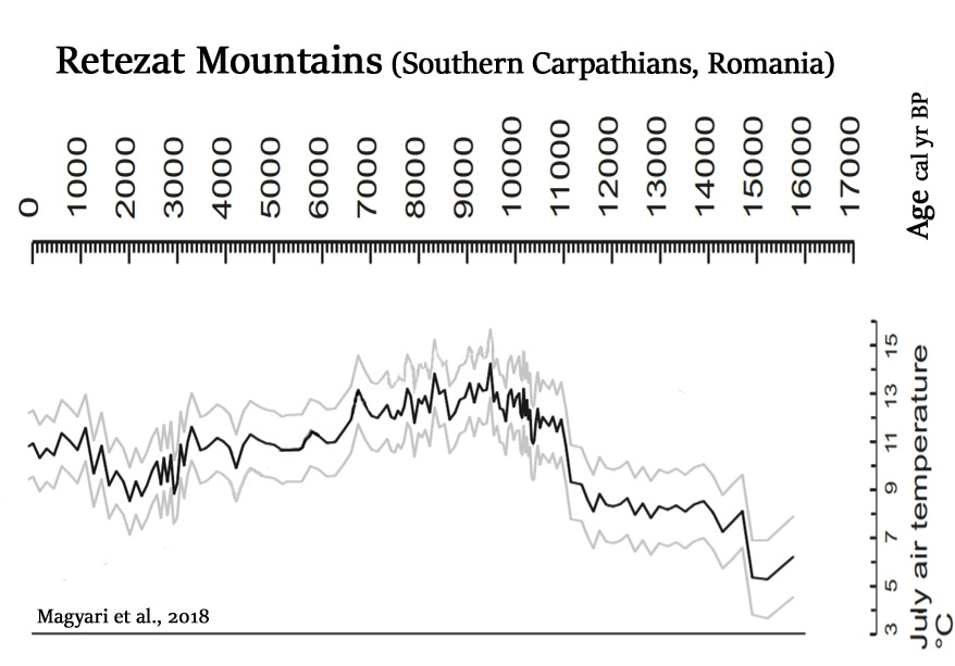
Magyari et al., 2018 [I]ts climatic tolerance limits were used to infer July mean temperatures exceeding modern values by 2.8°C at this time [8200-6700 cal yr BP] (Magyari et al., 2012).
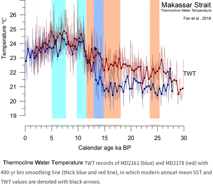
Fan et al., 2018 The thermocline water temperature variabilities of the two sites, in particular the highest peaks at ~7 ka BP, are different from the records of the open western Pacific. Reoccurrence of the South China Sea Throughflow and thus a decreased surface throughflow along the Makassar Strait perhaps led to a warmer peak of thermocline temperature at ~7 ka BP than at ~11 ka BP.
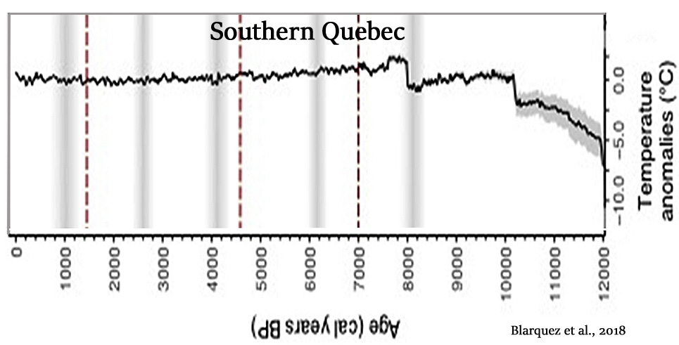
Blarquez et al., 2018
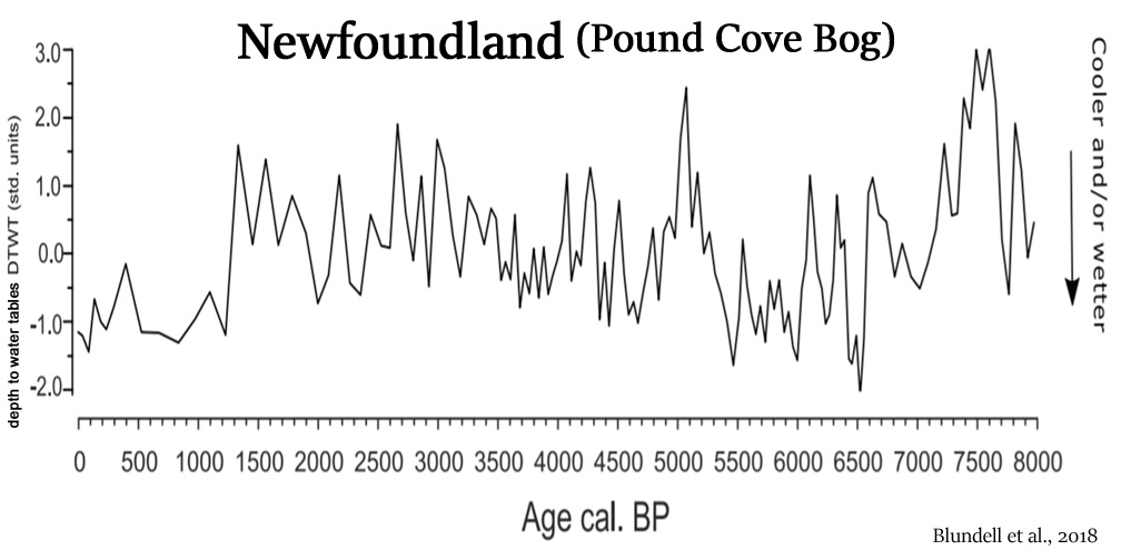
Blundell et al., 2018 Energy carried by warm tropical water, transported via the Atlantic Meridional Overturning Circulation (AMOC), plays a vital role in regulating the climate of regions bordering the North Atlantic Ocean. Previous phases of elevated freshwater input to areas of North Atlantic Deep Water (NADW) production in the early to mid-Holocene have been linked with slow-downs in the AMOC and changes in regional climate.
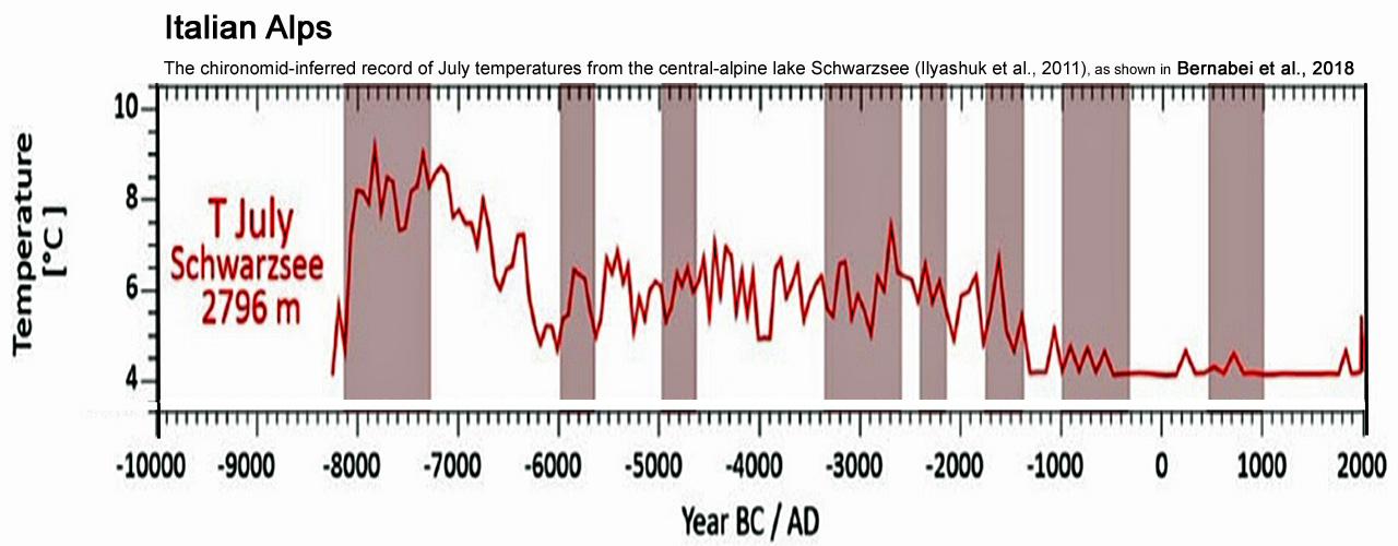
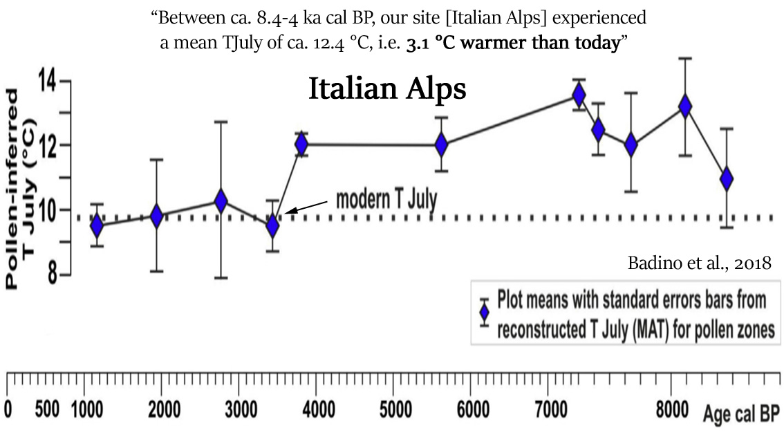
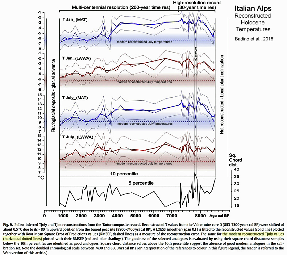
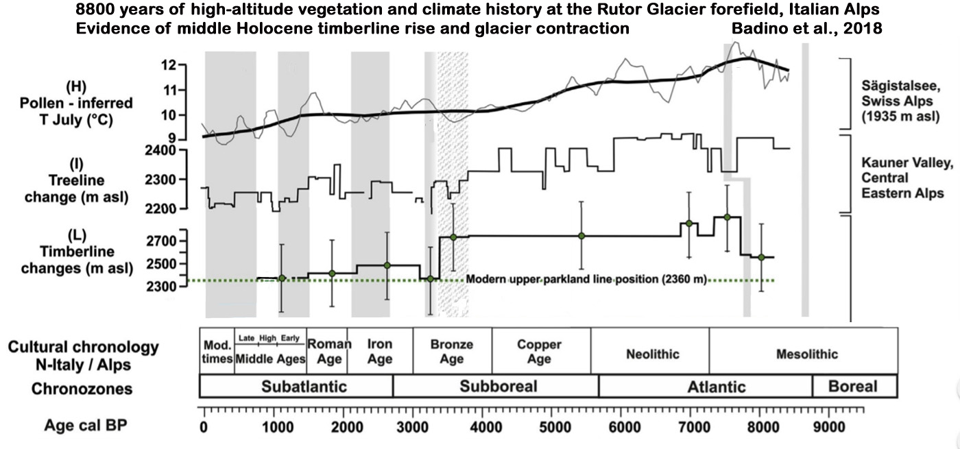
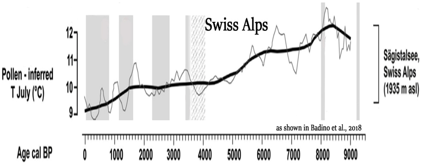
Badino et al., 2018 Between ca. 8.4-4 ka cal BP [8,400 to 4,000 years before present], our site [Italian Alps] experienced a mean TJuly of ca. 12.4 °C, i.e. 3.1 °C warmer than today [9.3 °C]. … Between 7400 and 3600 yrs cal BP, an higher-than-today forest line position persisted under favorable growing conditions (i.e. TJuly at ca. 12 °C).
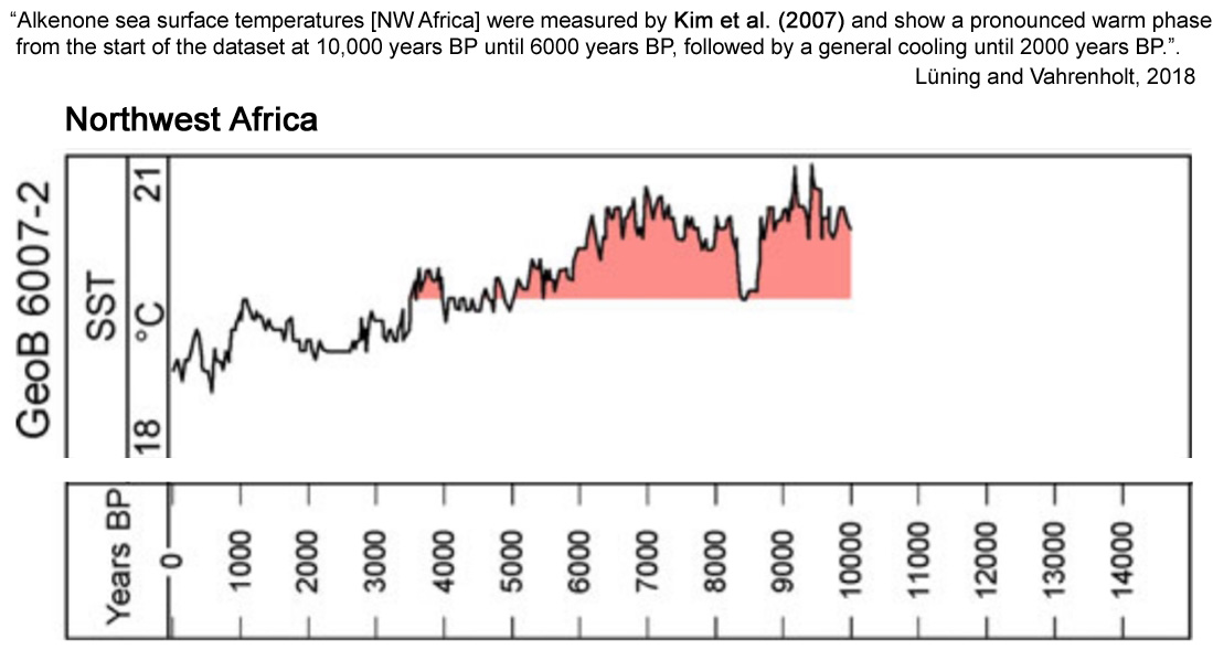
Lüning and Vahrenholt, 2018 The early Holocene ‘Green Sahara’ forms part of a long series of wet periods that have occurred over the past hundred thousand to million years in North Africa and Arabia. Notably, climate models are still unable to match the observed hydroclimatic changes in a quantitative way. Simulated rainfall during the African Humid Period over the Sahara is not sufficient to sustain vegetation at a level seen in the palaeo record, indicating that processes such as vegetation and dust feedbacks still need to be refined. Sea surface temperatures in North Africa and Arabia during the early Holocene were generally one to several degrees C warmer than during the late Holocene. Warming began around 12,000 years BP and ended around 5000 years BP. The warm period generally coincided with the early Holocene wet phase in the region and is linked to the Holocene Thermal Maximum, an early Holocene period during which temperatures were globally elevated. The review suggests that the Holocene climate history of North Africa and Arabia is closely linked to the global development and that significant temperature changes have also occurred in subtropical climate belts.
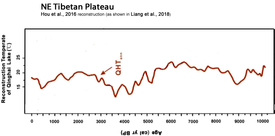
Liang et al., 2018
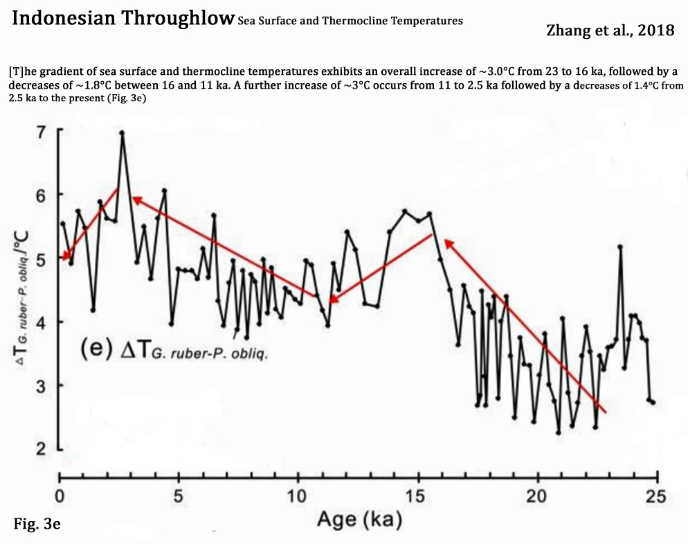
Zhang et al., 2018 [T]he gradient of sea surface and thermocline temperatures exhibits an overall increase of ~3.0°C from 23 to 16 ka, followed by a decreases of ~1.8°C between 16 and 11 ka. A further increase of ~3°C occurs from 11 to 2.5 ka followed by a decrease of 1.4°C from 2.5 ka to the present (Fig. 3e).
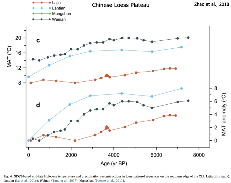
Zhao et al., 2018 According to the interpolation of meteorological data of the two nearest weather stations at Linxia (ca. 46 km away; MAT [mean annual temperature] = 7.3 °C) and Minhe (ca. 54 km away; MAT [mean annual temperature] = 8.3 °C)… In this study, we reconstructed mid-late Holocene climatic changes using GDGT distributions in a loess-paleosol sequence in the Lajia Ruins of the Neolithic Qijia Culture, Guanting Basin, in the southwestern end of the Chinese Loess Plateau. … MAT [mean annual temperature] decreased from 11.9 °C to 8.0 °C, during the past ca. 7000 yr, and a drastic decline in MAP [mean annual precipitation] (70 mm), accompanied by a 0.8 °C decline in MAT [mean annual temperature], occurred at 3800–3400 yr BP.
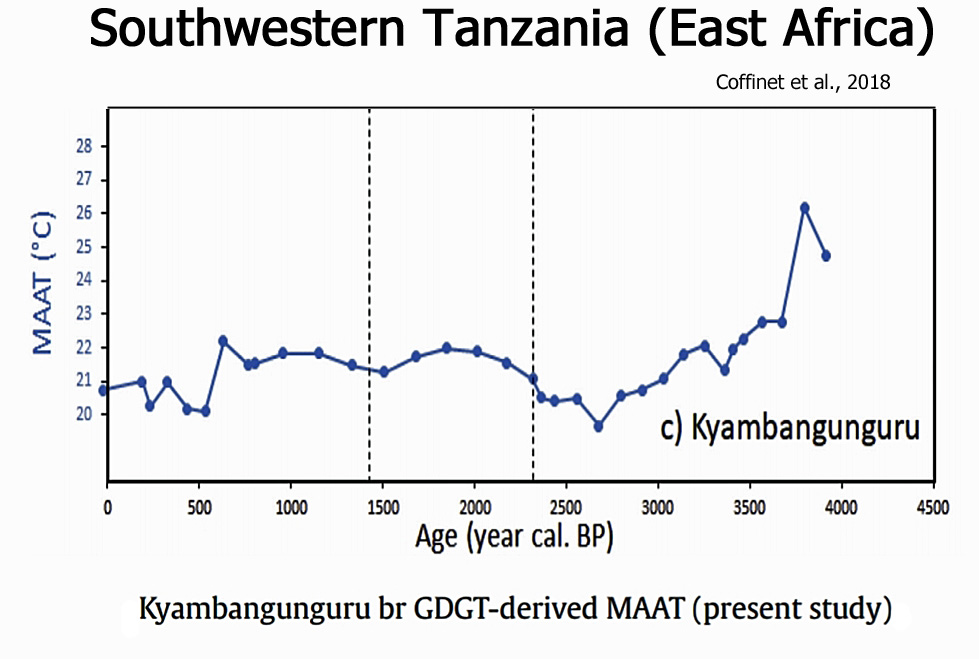
Coffinet et al., 2018 This study represents the first detailed late Holocene quantitative air temperature reconstruction from the RVP [Rungwe Volcanic Province, southwestern Tanzania/East Africa] region. We identified a succession of cold/warm/cold events, largely in phase with the other regional East African climate records and with the cold periods identified worldwide by Wanner et al. (2011). This further supports that global scale processes may be the main drivers of the Holocene climatic variability. Moreover, warm conditions during the MCA followed by abrupt cooling during the LIA were observed at Kyambangunguru and elsewhere in East Africa suggesting that these two recent events occurred globally.
Oswald et al., 2018
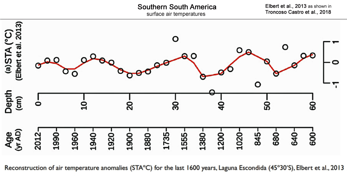
Troncoso Castro et al., 2018
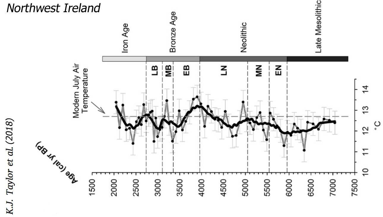
Taylor et al., 2018 This study provides the first mid to late Holocene chironomid-inferred temperature model for Ireland, creating a valuable climatic context for the development of Irish society during the Neolithic and Bronze Age. This reconstruction provides evidence of multiple fluctuations in temperature during the mid to late Holocene with a cold phase during the late Mesolithic (6800–5890 cal yr BP), followed by a warming period during the early Neolithic (5890–5570 cal yr BP). C-ITs reflect a relatively warm climate during the middle Neolithic, with a substantial warming from the late Neolithic into the early Bronze Age (4630–3810 cal yr BP), with temperatures registering above the modern day average between 3990 and 3810 cal yr BP.
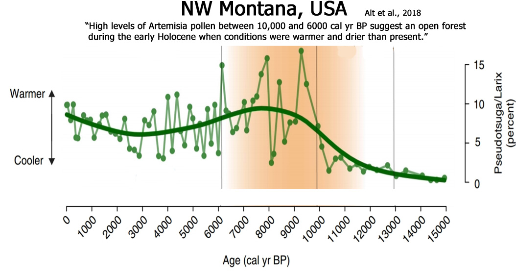
Alt et al., 2018 High levels of Artemisia pollen between 10,000 and 6000 cal yr BP suggest an open forest during the early Holocene when conditions were warmer and drier than present.
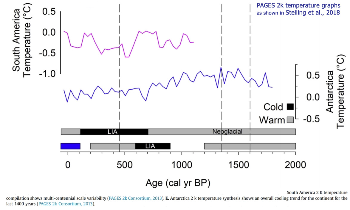
Stelling et al., 2018
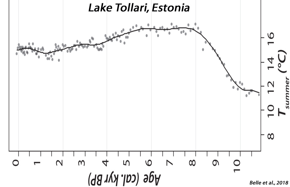
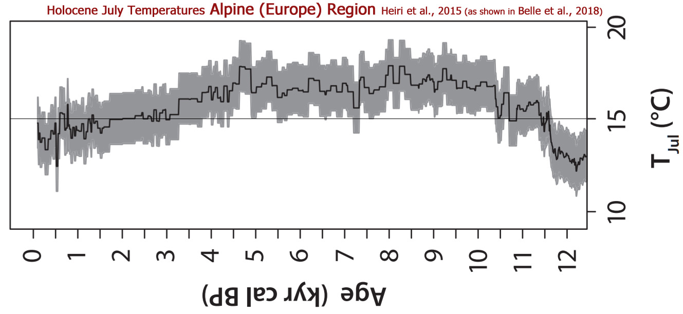
Belle et al., 2018 Comparable patterns of air temperature changes for the two studied areas have been reported for the Holocene (Figure 2, Heiri et al., 2015; Holmstrom, Ilvonen, Seppa, & Veski, 2015; Belle, Poska, et al., 2017). These patterns can be divided into three climatic periods: (1) from c. 11.7 to 8.2 kyr cal. BP (Early Holocene) when the Holocene coolest temperatures were observed, followed by a rapid warming, (2) maximal and stable temperatures during the Holocene thermal maximum (from c. 8.2 to 4.2 kyr cal. BP) and (3) since c. 4.2 kyr cal. BP (Late Holocene) when a slight gradual cooling was observed.
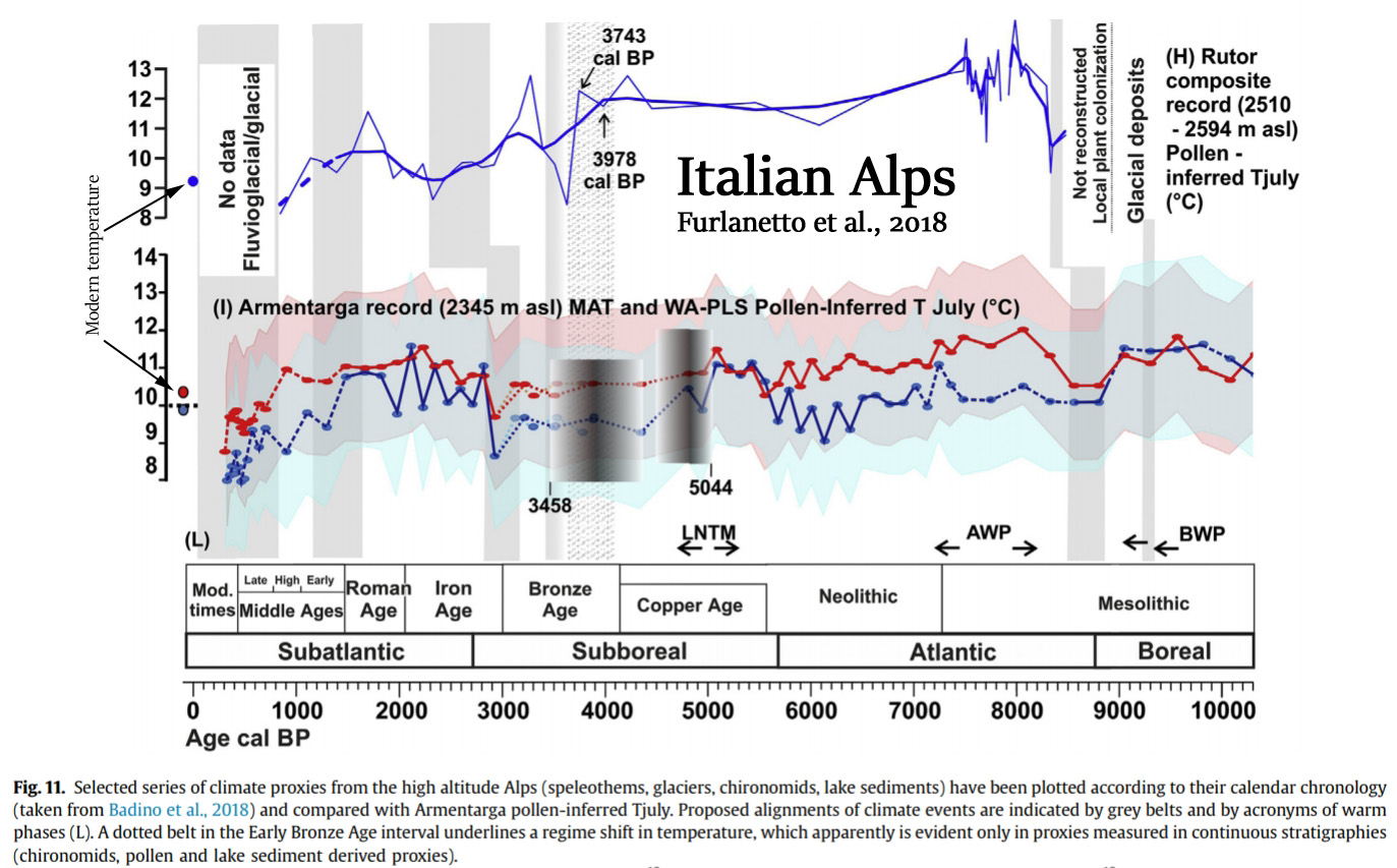
Furlanetto et al., 2018 [A] drop in temperature is documented in both reconstructions at around 2.9 ka cal BP in the Early Iron Age. After a warmer period around 2.8-1.5 ka cal BP, a new cooling trend appears from the Late Middle Age to Modern times in a phase of higher human impact
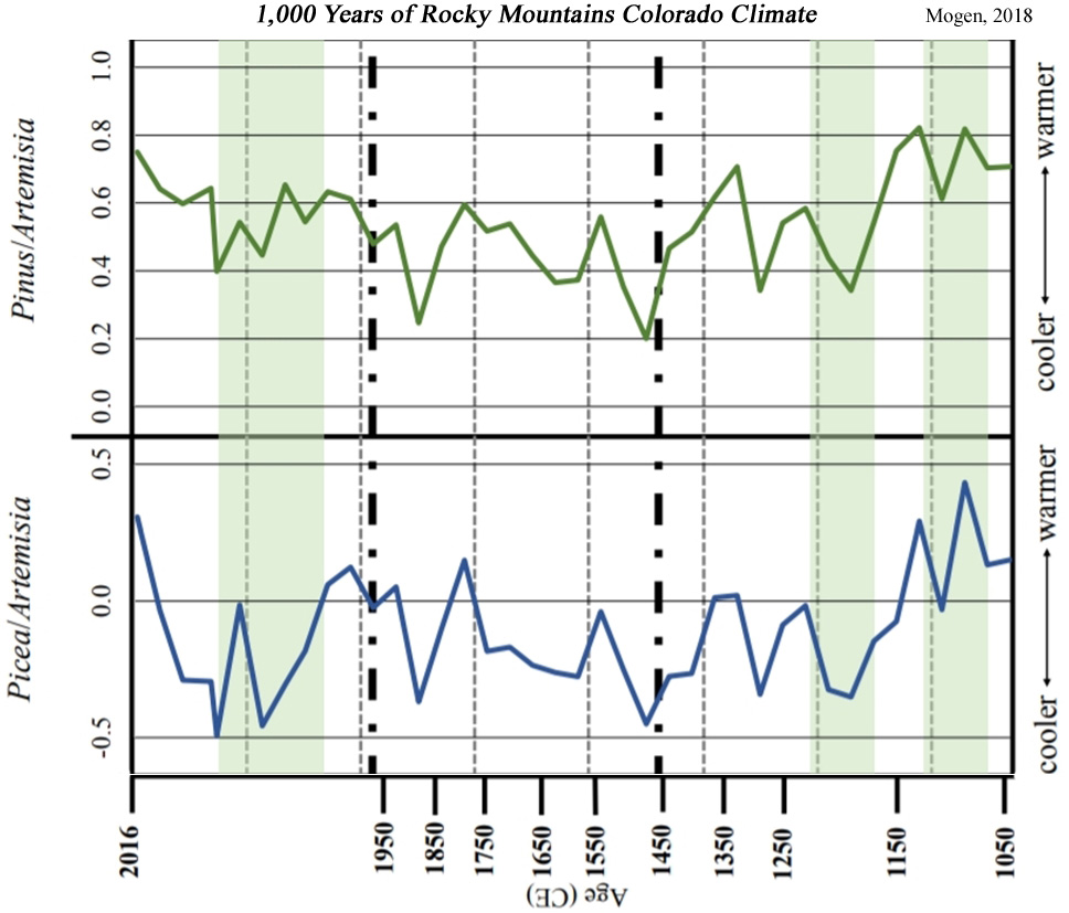
Mogen, 2018 Around 9 ka [9,000 years ago] average summer temperatures are estimated to have been over 2°C warmer than present, and between 10.4-6.6 ka treeline was about 80 m higher than present in the San Juan Mountains [Colorado, Rockies] (Elias et al., 1991; Carrara, 2011).
Bajolle et al., 2018
Papadomanolaki et al., 2018 (Baltic Sea) A large fraction of the Baltic Proper became hypoxic again between 1.4 and 0.7 ka BP, during the Medieval Climate Anomaly (MCA), when mean air temperatures were 0.9–1.4 °C higher than temperatures recorded in the period 1961–1990 (e.g. Mann et al., 2009; Jilbert and Slomp, 2013).
Leonard et al., 2018 (Great Barrier Reef, Australia) Coral derived sea surface temperature (SST-Sr/Ca) reconstructions demonstrate conditions ∼1 ◦C warmer than present at ∼6200 (recalibrated 14C) and 4700 yr BP, with a suggested increase in salinity range (δ18O) associated with amplified seasonal flood events, suggestive of La Niña (Gagan et al., 1998; Roche et al., 2014).
Suvorov and Kitov, 2018 (Eastern Sayan, Siberia) The authors examined the variability of activity of modern glaciation and variation of natural conditions of the periglacial zone on climate and on dendrochronological data. Results of larch and Siberian stone pine growth data were revealed at the higher border of forest communities. … It is believed that the temperature could be 3.5 °C warmer at the Holocene optimum than at the present time (Vaganov and Shiyatov 2005). … Since 2000, there has been growth of trees instability associated with a decrease in average monthly summer temperatures. … Since the beginning of 2000, decrease in summer temperatures was marked.
Lozhkin et al., 2018 (East Siberia) The postglacial occurrence of relatively warm/dry and warm/wet intervals is consistent with results of a regional climate‐model simulation that indicates warmer than present temperatures and decreased effective moisture at 11 000 cal. a BP and persistence of warm conditions but with greater moisture and longer growing season at 6000 cal. a BP.
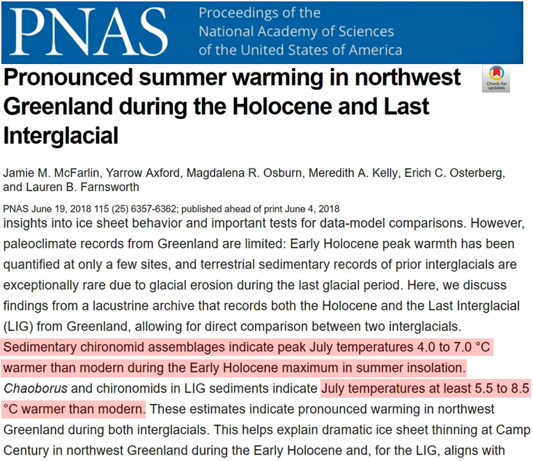
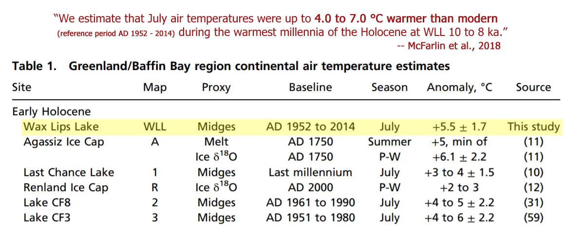
Smith, 2018 (Greenland Ice Sheet) To project how much sea level will rise in response to ongoing climate warming, one of the things we need to know is how sensitive the rate of Greenland Ice Sheet melting is to rising temperatures. McFarlin et al. present results from a set of sediment cores from a small nonglacial lake in the highlands of northwest Greenland, which contain deposits from the Holocene and the Last Interglacial (LIG). They found midge assemblages indicating peak July temperatures that were 4.0° to 7.0°C warmer than modern temperatures during the early Holocene and at least 5.5° to 8.5°C warmer during the LIG. This perspective of extreme warming suggests that even larger changes than predicted for this region over the —–coming century may be in store.
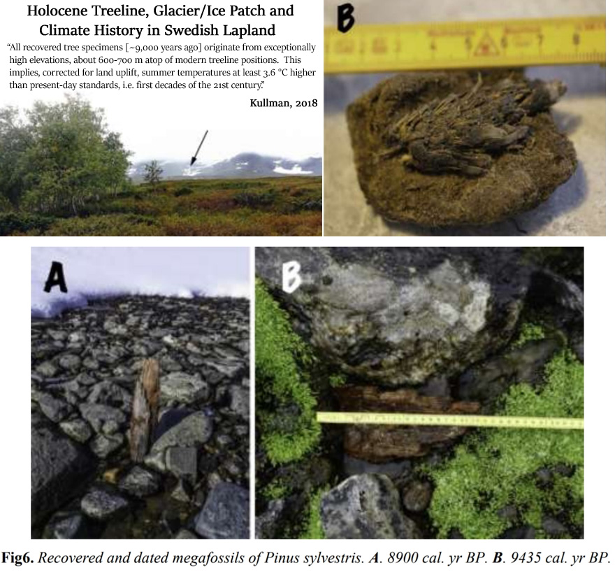
Kullman, 2018 (Scandes, Northern Sweden) The present paper reports results from an extensive project aiming at improved understanding of postglacial subalpine/alpine vegetation, treeline, glacier and climate history in the Scandes of northern Sweden. The main methodology is analyses of mega fossil tree remnants, i.e. trunks, roots and cones, recently exposed at the fringe of receding glaciers and snow/ice patches. This approach has a spatial resolution and accuracy, which exceeds any other option for tree cover reconstruction in high-altitude mountain landscapes. … All recovered tree specimens originate from exceptionally high elevations, about 600-700 m atop of modern treeline positions. … Conservatively drawing on the latter figure and a summer temperature lapse rate of 0.6 °C per 100 m elevation (Laaksonen 1976), could a priori mean that, summer temperatures were at least 4.2 °C warmer than present around 9500 year before present. However, glacio-isostatic land uplift by at least 100 m since that time (Möller 1987; Påsse & Anderson 2005) implies that this figure has to be reduced to 3.6 °C higher than present-day levels, i.e. first decades of the 21st century. Evidently, this was the warmth peak of the Holocene, hitherto. This inference concurs with paleoclimatic reconstructions from Europe and Greenland (Korhola et al. 2002; Bigler et al. 2003; Paus 2013; Luoto et al. 2014; Väliranta et al. 2015).
Borisova, 2018 (central East European Plain) Paleobotanical assemblages from peat, lake, and archaeological deposits reveal that during the Middle Holocene (MH; ca. 9.0 to 4.7 kyr BP), the central East European Plain was occupied by highly productive and diverse mixed-oak forests, along with mire, meadow, and riverine communities. Climatic reconstructions based on modern analogues of fossil pollen and plant macrofossil assemblages indicate that throughout the MH [Middle Holocene] mean annual precipitation was at near present levels (~600 mm) and July temperatures were similar to those of today (~17°C). However, differences in the Fossil Floras (FFs) suggest changes in winter conditions though the MH [Middle Holocene, 9.0 to 4.7 kyr BP], with January temperatures higher than the present-day value of -10°C by 2°C in the Early Atlantic, 6°C in the Middle Atlantic, and 3°C in the Late Atlantic-Early Subboreal. The annual frost-free period was 15 days longer than today in the Early Atlantic, about one month longer in the Late Atlantic, and became close to present by the beginning of the Subboreal. The combination of warm winters with diverse and productive vegetation communities provided an environment that was more hospitable than that of today for Late Mesolithic and Neolithic societies.
McFarlin et al., 2018 (Greenland) Early Holocene peak warmth has been quantified at only a few sites, and terrestrial sedimentary records of prior interglacials are exceptionally rare due to glacial erosion during the last glacial period. Here, we discuss findings from a lacustrine archive that records both the Holocene and the Last Interglacial (LIG) from Greenland, allowing for direct comparison between two interglacials. Sedimentary chironomid assemblages indicate peak July temperatures [Greenland] 4.0 to 7.0 °C warmer than modern during the Early Holocene maximum [10,000 to 8,000 years ago] in summer insolation. Chaoborus and chironomids in LIG sediments indicate July temperatures at least 5.5 to 8.5 °C warmer than modern.
Bartels et al., 2018 (North Atlantic Region) During summer, AW [Atlantic Water] rises up to waterdepths as shallow as ~55 m. … Summer surface temperatures [1955-2012] range between up to 3°C at the northern mouth and <-1.5 °C at the southern mouth of the Hinlopen Strait, while winter surface temperatures vary between 0.5 and <~1.5°C (averaged, 1955–2012; Locarnini et al. 2013). … Increased summer insolation probably amplified the surface melting of the glaciers resulting in enhanced meltwater production and in a very high accumulation of finegrained sediments within the fjord […]. In addition, during the mild early Holocene conditions, summer sea-surface temperatures probably reaching 8–10°C [~5 – 9.5°C warmer than 1955-2012] (indicated by M. edulis findings as discussed in Hansen et al. 2011) may have contributed to reducing the number of glaciers that entered the fjord directly as tidewater glaciers and thus causing a diminished IRD input. These comparably warm surface temperatures most likely resulted in a reduced sea ice cover during summer, which is also reflected in the sea-ice biomarker data exhibiting lowest IP25 values during the early Holocene. … [G]lacier advances are most likely caused by atmospheric cooling as indicated, e.g. by d18O values from the Greenland NGRIP ice-core (Rasmussen et al. 2014a), by data from peats and permafrost soils on Spitsbergen (e.g. Humlum et al. 2003; Humlum 2005; Jaworski 2016), and by evidence that solar activity reduced around 2.7 ka, contributing to a cooling in both hemispheres (van Geel et al. 1999, 2000). … In lake sediments from northwestern Spitsbergen a temperature drop of ~6°C is recorded between c. 7.8 and c. 7 ka [-0.8°C per century], which has been connected to a stronger influence of Arctic Water and expanding sea ice (van der Bilt et al. 2018).
Street-Perrot et al., 2018 (Estonia) Estimates of summer temperatures in Estonia based on rapidly responding proxies such as aquatic macrofossils (Valiranta et al., 2015) and chironomids (Heiri et al., 2014) suggest conditions 2 °C warmer than today during the early Holocene.
Pozachenuk, 2018 (Western Russia) Mass peat accumulation in the territory of Vyatka region began only in the first half of the Atlantic Holocene period. The maximum warming corresponds to the second half of at (climatic optimum Holocene), when the average temperatures of January and July exceeded modern 2-3˚C. at this time in the region formed coniferous-broad-leaved forests of complex composition, with a slight presence of broad-leaved species (Qercus, Tilia, Ulmus) and Corulus. Siberian element of flora-fir on the territory of Vyatka region appeared only in the Subatlantic period of Holocene, most likely due to climatic conditions.
Kolaczek et al., 2018 (Southeastern Poland) The reconstruction of the mean July temperature based on Chironomidae revealed the exceptionally high rate of warming during the period of ca. 11,490–11,460 cal. BP (at least 1 °C per decade) up to values > 2 °C than modern ones. … Between ca. 11,490 and 11,460 cal. BP, the strongest warming trend in the Early Holocene MJT was registered, that is from 15 to 20.7°C (0.19°C yr1, 1.9°C/decade). Then, ca. 11,450 cal. BP, the temperature decreased to 18.3°C and up to ca. 10,560 cal. BP MJT fluctuated between 17 and 19°C. The climate of the area [today] is classified as cold temperate with mean annual air temperature of 8.2°C and mean annual precipitation 620 mm. A mean temperature of the warmest month, i.e. July, is +18.2°C [today], whereas a mean temperature of the coldest month, i.e. January, is -3.6°C.
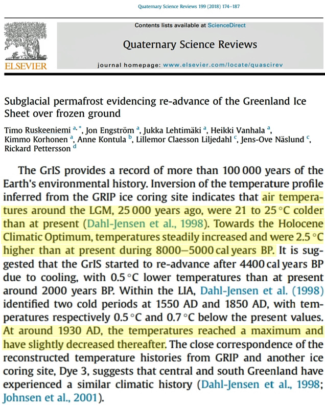
Ruskeeniemi et al., 2018 (Greenland Ice Sheet) Towards the Holocene Climatic Optimum, temperatures steadily increased and were 2.5°C higher than at present during 8000-5000 cal years BP. It is suggested that the GrIS started to re-advance after 4400 cal years BP due to cooling, with 0.5°C lower temperatures than at present around 2000 years BP. Within the LIA, Dahl-Jensen et al. (1998) identified two cold periods at 1550 AD and 1850 AD, with temperatures respectively 0.5°C and 0.7°C below the present values. At around 1930 AD, the temperatures reached a maximum and have slightly decreased thereafter.
Leopold et al., 2018 (Arctic Svalbard) [T]he summer SSTs today around Svalbard are some 5–8 °C lower than during the thermal peak of the early Holocene.
Voldstad, 2018 (Arctic Svalbard) The early record of thermophilous species not commonly distributed around Svalbard today is in line with the description of a first Holocene warm period in Svalbard with climate about 6°C warmer than present between 10 and 9,2 cal. ka BP (Mangerud & Svendsen 2018).
Clarke et al., 2018 (Fennoscandia) Early Holocene climate in northern Fennoscandia was affected by summerinsolation that was higher than present (Berger 1978; Berger&Loutre 1991). … [P]ollen-based summer temperature reconstructions indicate July temperatures of +1.5 +/- 0.5 °C above modern (1961–1990) values in northern Fennoscandia during the regional HTM identified at c. 8000–6000 cal. a BP (Møller & Holmeslet 2002; Jensen & Vorren 2008; Seppa et al. 2009; Sejrup et al. 2016).
Oxenham et al., 2018 (China) Several sources of proxy data demonstrate that significant temperature rises (the Holocene Thermal Maximum) occurred between 11 000 and 5000ya [years ago], peaking 7200–6000ya in China, where surface temperatures were 1–4°C higher and rainfall 40–100 per cent greater than today (Tao et al. 2010; Renssen et al. 2012). … Da But and Dingsishan communities [China] were adapting to optimal hunter-gatherer conditions probably mediated by the Holocene Thermal Maximum. They lived in a climate warmer than now, which presumably favoured the growth and spread of economically valuable plants, such as Canarium, sago and root crops, in quantities that could sustain large sedentary hunter-gatherer populations. … Following the Holocene Thermal Maximum, lower sea levels, coastal progradation (orseaward extension of the coast) and declining temperature and rainfall presumably had a negative impact on these communities and their resources.
Clark et al., 2018 (South China) Evidence from the fossil coral record has shown that coral assemblages were able to extend their geographical range to higher latitudes during past global warming events. In the face of future global warming scenarios, we investigate the potential for China’s subtropical coral communities to act as a refuge for corals as ocean temperatures continue to warm. Using uranium-thorium dating to chronologically constrain the age of dead corals, we reveal two distinct periods of coral growth between 6.85 and 5.51 ka B.P. and 0.11 to –0.05 ka B.P. (relative to A.D. 1950). The former coincides with the mid–Holocene Warm Period when temperatures in South China were ~1–2 °C warmer than present.
Lack Of Anthropogenic/CO2 Signal In Sea Level Rise
Duvat et al., 2018 This review first confirms that over the past decades to century, atoll islands exhibited no widespread sign of physical destabilization by sea-level rise. The global sample considered in this paper, which includes 30 atolls and 709 islands, reveals that atolls did not lose land area, and that 73.1% of islands were stable in land area, including most settled islands, while 15.5% of islands increased and 11.4% decreased in size. Atoll and island areal stability can therefore be considered as a global trend. Importantly, islands located in ocean regions affected by rapid sea-level rise showed neither contraction nor marked shoreline retreat, which indicates that they may not be affected yet by the presumably negative, that is, erosive, impact of sea-level rise. .. These results show that atoll and island areal stability is a global trend, whatever the rate of sea-level rise. Tuvaluan atolls affected by rapid sea-level rise (5.1 mm/yr; Becker et al., 2012) did not exhibit a distinct behavior compared to atolls located in areas showing lower sea-level rise rates, for example, the Federated States of Micronesia or Tuamotu atolls.
Mörner, 2018 It is a serious mistake to claim that global sea level is in a phase of rapid rise. Observationally based facts document a present changes in absolute (eustatic) sea level ranging between ±0.0 and +1.0 mm/yr. This poses no threats what so ever. In New York City, sea level is rising at a rate of +2.84 mm/yr, which would imply an additional rise in sea level by 23.3 cm by 2100, a modest rise that can be handled without problems. There also occur statements that sea level may raise by 1 m or more by 2100. All such claims represent fake news that does not concur with observational fact and violates physical frames of realism.
Khan, 2018 [T]hermal expansion only explains part (about 0.4 mm/yr) of the 1.8 mm/yr observed sea level rise of the past few decades. However, observation claim of 1.8 mm/yr sea level rise is also limited in scope and accuracy. … Claim and prediction of 3 mm/yr rise of sea-level due to global warming and polar ice-melt is definitely a conjecture. … Prediction of 4–6.6 ft sea level rise in the next 91 years between 2009 and 2100 is highly erroneous. … Hence, both regional and local sea-level rise and fall in meter-scale is related to the geologic events only and not related to global warming and/or polar ice melt. … In conclusion, global warming, both polar and terrestrial ice melts, and climate change might be a reality but all these phenomena are not related to sea level rise and fall.
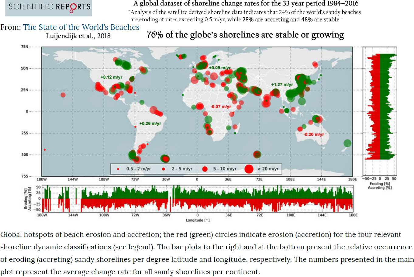
Luijendijk et al., 2018 The application of an automated shoreline detection method to the sandy shorelines thus identified resulted in a global dataset of shoreline change rates for the 33 year period 1984–2016. Analysis of the satellite derived shoreline data indicates that 24% of the world’s sandy beaches are eroding at rates exceeding 0.5 m/yr, while 28% are accreting and 48% are stable. …. Erosion rates exceed 5 m/yr along 4% of the sandy shoreline and are greater than 10 m/yr for 2% of the global sandy shoreline. On the other hand, about 8% of the world’s sandy beaches experience significant accretion (>3 m/yr), while 6% (3%) are accreting more than 5 m/yr (10 m/yr). … Taking a continental perspective, Australia and Africa are the only continents for which net erosion (−0.20 m/yr and −0.07 m/yr respectively) is found, with all other continents showing net accretion.
Parker, 2018 Conclusion: The tide gauges of China are too short, or incomplete, to permit a proper assessment of the long-term trend, more than for the slope, certainly for the acceleration. … There is no clear evidence the sea levels of China are rising at an accelerating rate because of thermal expansion and mass addition, as the data available is either insufficient or conflicting. Conclusions about the sea levels of China may only be drafted from all the local relative rates of rise, and the global relative rates of rise and accelerations of different data sets. The slopes for the tide gauges of China and the slopes and accelerations for the worldwide tide gauges suggest that the coastal mean relative sea level in the China Seas very likely rises from −1 to 3 mm/year in the past half century and it may likely rise of 0–0.259 m in the twenty-first century.
Tomasicchio et al., 2018 The estimation of long-term sea level variability is of primary importance for a climate change assessment. Despite the value of the subject [sea level changes], no scientific consensus has yet been reached on the existing acceleration in observed values. … The Intergovernmental Panel on Climate Change (IPCC), an international organisation responsible for assessing the scientific basis of climate change, its impacts and future risks, warned that at current trends, the projected increments in mean sea level (MSL) for the year 2100, relative to the 1986–2005 period [IPCC] are 400, 470, 480 and 630 mm, for the Representative Concentration Pathways scenarios indicated as RCP2.6, RCP4.5, RCP6.0 and RCP8.5, respectively. However, from the tide gauge records, the acceleration required to reach these large projected MSL [mean sea level] rises over the course of the twenty-first century is not evident. Even though the measurement of this acceleration is a topic with a long standing history (Douglas 1991; Church and White 2006; Jevrejeva et al. 2008), the most recent debate was initiated by a series of publications (Houston and Dean 2011a, b, c, d, e) that raised concerns about the general validity of the sea level projections; the authors did not find any acceleration in the sea level in USA tide gauge records during the twentieth century. Instead, for each time period they considered, the records showed small decelerations that are consistent with a number of earlier studies of worldwide gauge records (Woodworth 1990; Douglas 1992; Woodworth et al. 2009). By using a different approach in data analysis, other researchers (Rahmstorf and Vermeer 2011a, b; Donoghue and Parkinson 2011a, b) found the arguments of Houston and Dean (2011a, b, c, d, e) not convincing and showed that accelerations are present.
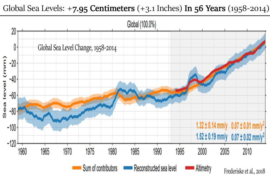
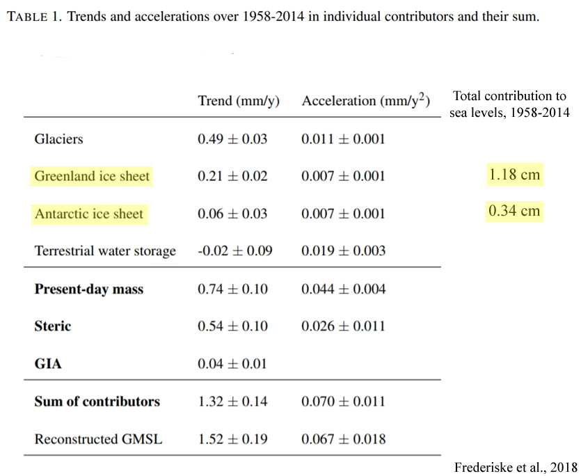
Frederiske et al.,2018 For the first time, it is shown that for most basins the reconstructed sea level trend and acceleration can be explained by the sum of contributors, as well as a large part of the decadal variability. The global-mean sea level reconstruction shows a trend of 1.5 ± 0.2 mm yr−1 over 1958–2014 (1σ), compared to 1.3 ± 0.1 mm yr−1for the sum of contributors.
[Global sea levels rose 3.1 inches (1.4 mm/yr) between 1958-2014, with 0.59 of an inch meltwater contribution from the Greenland and Antarctic ice sheets combined.]
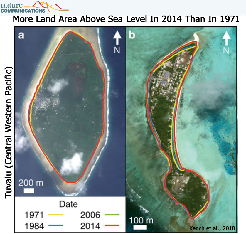
Kench et al., 2018 We specifically examine spatial differences in island behaviour, of all 101 islands in Tuvalu, over the past four decades (1971–2014), a period in which local sea level has risen at twice the global average (Supplementary Note 2). Surprisingly, we show that all islands have changed and that the dominant mode of change has been island expansion, which has increased the land area of the nation. … Using remotely sensed data, change is analysed over the past four decades, a period when local sea level has risen at twice the global average [<2 mm/yr-1] (~3.90 ± 0.4 mm.yr−1). Results highlight a net increase in land area in Tuvalu of 73.5 ha (2.9%), despite sea-level rise, and land area increase in eight of nine atolls.
Ahmed et al., 2018 This paper draws upon the application of GIS and remote sensing techniques to investigate the dynamic nature and management aspects of land in the coastal areas of Bangladesh. … This research reveals that the rate of accretion [coastal land growth] in the study area is slightly higher than the rate of erosion. Overall land dynamics indicate a net gain of 237 km2 (7.9 km2annual average) of land in the area for the whole period from 1985 to 2015.
Parker et al., 2018 The anomalous pattern of relative sea levels for the Samoan Islands that followed the 2009 earthquake and tsunami is explained by coupling tide-gauge time series of relative sea levels and GPS time series of absolute geocentric positions of inland fixed domes. The subsidence of the land is responsible for the relative sea level acceleration that followed the earthquake. The pattern of subsidence is characterized by small departures from a linear pattern immediately before the earthquake, an abrupt change at the earthquake, and then a parabolically reducing extra subsidence. The absolute geocentric sea levels obtained clearing the relative sea level signal of the subsidence signal are stable. There is a need to couple GPS monitoring of tide gauge position with tide gauge measurements of relative sea levels without any linearity assumption to produce reliable, accurate, assessments of the pattern of sea level rise to inform policy makers.
Hisabayashi et al., 2018 Summary: Atoll islands are low-lying accumulations of reef-derived sediment that provide the only habitable land in Tuvalu, and are considered vulnerable to the myriad possible impacts of climate change, especially sea-level rise. This study examines the shoreline change of twenty-eight islands in Funafuti Atoll between 2005 and 2015 … Most of the islands remained stable, experiencing slight accretion or erosion or a combination of both over time. The total net land area of the islands increased by 1.55 ha (0.55%) between 2005 and 2010, and it has decreased by 1.90 ha (0.68%) between 2010 and 2015, resulting in a net decrease by 0.35 ha (0.13%). … Results indicate a 0.13% (0.35 ha) decrease in net island area over the study time period, with 13 islands decreasing in area and 15 islands increasing in area. Substantial decreases in island area occurred on the islands of Fuagea, Tefala and Vasafua, which coincides with the timing of Cyclone Pam in March, 2015.
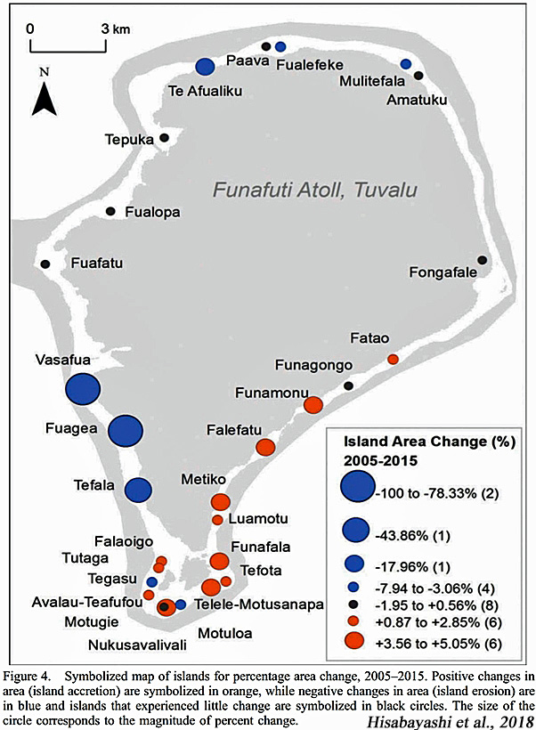
Parker, 2018 Regionally, the sea levels in the PRD [Pearl River Delta, China] region and Japan show no significant acceleration from 1900 to present, but only oscillations. This result is consistent with the other coastal area of the world where long-term tide gauges are located. Policy making, and management, should therefore focus on adaptive measures linked to the monitoring by tide gauges and Global Navigation Satellite System (GNSS) of relative sea level rise and land subsidence. Extreme sea level rise warnings based on predictions by never validated models, or speculations, that are defocusing coastal management from every other relevant situation, should be discharged. … [T]he long-term tide gauges of the world show no significant sign of sea level acceleration since the start of the 20th century… Ocean and coastal management in the area should be based on the accurate monitoring of the relative sea level rise and the subsidence of the land by coupled tide gauge and Global Navigation Satellite System measurements, rather than models’ predictions and speculations defocusing coastal management from more relevant situations than the non-existent threat of extreme sea level rise.
Schuerch et al., 2018 On the basis of our simulations, we find that, globally, rather than losses, wetland gains of up to 60 per cent of the current area are possible, if more than 37 per cent (our upper estimate for current accommodation space) of coastal wetlands have sufficient accommodation space, and sediment supply remains at present levels. … [M]ost large-scale assessments have overestimated the vulnerability of coastal wetlands to SLR [present-day sea level rise]. These differences highlight a major knowledge gap in our understanding of the responses of coastal wetland areas to global environmental change. It has been argued that the reason for the observed discrepancy is that large-scale assessments have so far failed to consider the well understood biophysical feedback mechanisms that are typically included in local-scale models. These mechanisms include the ability of coastal wetlands to build up vertically by sediment accretion, which is enhanced with increasing inundation heights and frequencies, triggered, for example, by accelerating SLR [present-day sea level rise], and which enables coastal wetlands to persist or even prosper with SLR [present-day sea level rise].
(press release) Rising sea levels don’t have to spell doom for the world’s coastal wetlands. A new study suggests salt marshes and other wetlands could accumulate soil quickly enough to avoid becoming fully submerged — if humans are willing to give them a little elbow room. … The new study builds on previous work that suggests rising seas will increase sediment buildup in some parts of coastal wetlands. This increased sediment, as well as human adaptations to allow wetlands to move inland as the seas rise, could allow the coastal fringes to not only survive but to increase their global area by as much as 60 percent.
Han et al., 2018 Previous studies suggest that anthropogenic warming has affected the multi-decadal trend patterns of sea level over the Indian Ocean (IO). This effect, however, has not been quantified. Using observational datasets combined with large ensemble experiments from two climate models, this paper assesses the effects of natural internal variability versus external forcing on the observed, multi-decadal trend pattern and the decadal sea level anomaly (SLA) of the IO since the 1960s. Because the global mean sea level rise (SLR), which results largely from external forcing, has been removed before the examination, the paper focuses on the regionally uneven distribution of trend and SLA. The impacts of climate modes are quantified using a Bayesian Dynamic Linear Model. For the regional trend pattern of 1958–2005, the effects of internal variability dominate external forcing. Over the Seychelles area where sea-level variations obtain the maximum, internal variability (external forcing) contributes 81% (19 ± 2.4%) of the observed trend. For decadal SLA, internal variability is the predominant cause, with a standard deviation (STD) ratio of externally forced/observed SLA being 18 ± 17% over Seychelles and 17 ± 11% near the Indonesian Throughflow (ITF) area. Climate modes account for most observed SLA during boreal winter, with the total effects of decadal ENSO, Indian Ocean Dipole (IOD), and monsoon accounting for 78–86% of the observed STD near the Seychelles region, ITF area, and coasts of Sumatra and the Bay of Bengal. … Over the North IO, the sea level experienced basin-wide falls from 1993–2003 but sharp rises from 2004–2013 [19,20]. Both observational analyses and OGCM experiments suggest that the surface wind over the IO is the primary cause for the observed decadal sea level variability [19,20,21,22], with the ITF making significant contributions primarily in the southeast tropical IO [21,23]. Thermosteric sea level is the primary contributor [22,24,25], with the halosteric sea level having apparent influence in some regions [22], such as the tropical southeast IO [26]. While surface wind associated with natural internal variability is suggested to be the major cause for decadal sea level variability [5,27], the effect of external forcing on regional, decadal sea-level variations over the IO remains unknown.
Mörner et al., 2018 Tide-gauges offer records of the relative changes in sea level. Out of a total of about 2300 stations (PSMSL), “a global set of ~300 tide gauges that serves as the backbone of the global in situ sea level network” in the Global Sea Level Observing System (GLOSS). There is no objective, straightforward solution for estimating a global mean value. The University of Colorado chose 184 global tide-gauge records. Their rate of distribution has a marked peak in the zone from ±0.0 to +2.0 mm/yr with a mean value at +1.14 mm/yr. Because the majority of stations used include a component of regional subsidence and local sediment compaction, the true mean sea level value should be <+1.14 mm/yr. … Satellite altimetry is a new and important tool, which reconstructs the entire ocean surface changes. But nowhere do the measurements agree with coastal observations. Satellite altimetry exceeds tide-gauge records by about 300%. There have even been accusations of data manipulation [Mörner, 2018].
Garner et al. (2017) propose SLR of up to 2.6 m by 2100, 10.5 m by 2200, and 17.5 m by 2300 (Fig. 1). These SLRs are far greater than those that occurred during catastrophic melting of immense ice sheets at the end of the Pleistocene, so the question arises, where will all the water come from to produce these very large SLRs? Melting of small, temperate, alpine glaciers wouldn’t produce anywhere near the SLRs projected by Garner et al., so the only possible sources of water are the Antarctic and Greenland ice sheets. The projections of Garner et al. of SLR of 7–8 m per century would require about seven times the end of the Pleistocene SLR when immense ice sheets were collapsing under warming of up to 20 °F in less than a century. To get these huge SLRs would require melting of an immense amount of ice from the Antarctic ice sheet. The average winter temperature in Antarctica is about –55 °F and temperatures have reached as low as 135 °F, so any significant melting of the Antarctic ice sheet would require 55° + 32° = 87 °F of warming just to get to the freezing point plus another 10 degrees or so to melt much ice. So Antarctica would have to warm up by 90–100 °F to melt enough ice to substantially raise sea level.
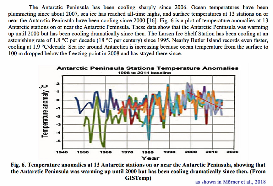
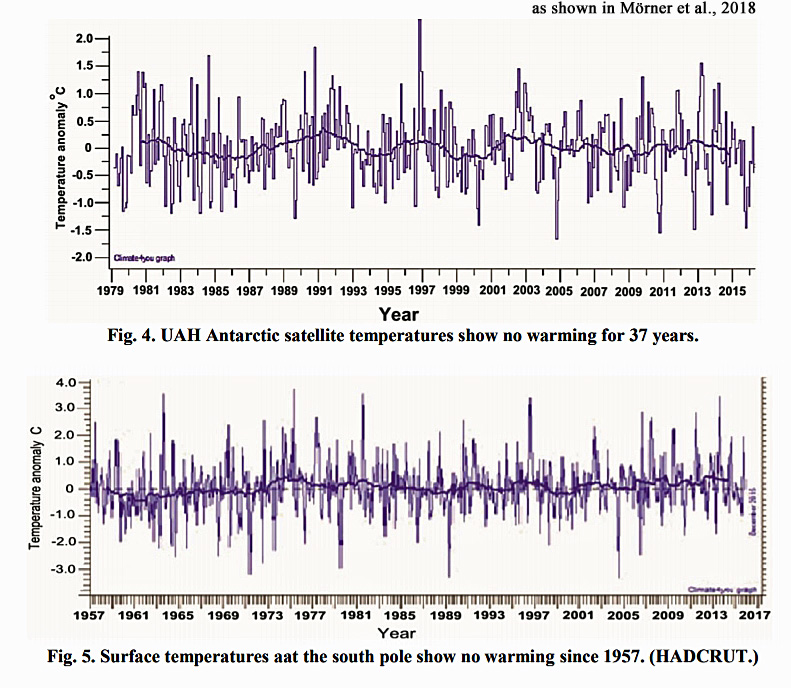
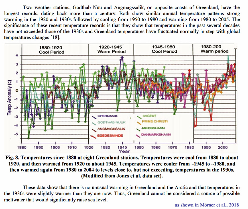
Piecuch et al., 2018 Here we analyse instrumental data and proxy reconstructions using probabilistic methods to show that vertical motions of Earth’s crust exerted the dominant control on regional spatial differences in relative sea-level trends along the US East Coast during 1900–2017, explaining most of the large-scale spatial variance. Rates of coastal subsidence caused by ongoing relaxation of the peripheral forebulge associated with the last deglaciation are strongest near North Carolina, Maryland and Virginia. Such structure indicates that Earth’s elastic lithosphere is thicker than has been assumed in other models. We also find a substantial coastal gradient in relative sea-level trends over this period that is unrelated to deglaciation and suggests contributions from twentieth-century redistribution of ice and water. Our results indicate that the majority of large-scale spatial variation in long-term rates of relative sea-level rise on the US East Coast is due to geological processes that will persist at similar rates for centuries. … We note that negative VLM [vertical land motion] reflects subsidence and hence contributes to sea-level rise. Correspondingly, the most negative VLM [vertical land motion] rate (−2.5 ± 0.6 mm yr−1) is likely (P = 0.75) to occur in the states that host the maximum sea-level rise, North Carolina or Virginia, whereas the most positive rate of VLM (0.7 ± 0.8 mm yr−1) is very likely (P = 0.90) to occur in Maine (Fig. 1g).
Sea Levels Multiple Meters Higher Than Present 4,000-7,000 Years Ago
Escobar-Torrez et al., 2018 (W Borneo, South China Sea) The predictions for a range of earth models show RSL [relative sea level] rising steeply up to 7000 yr BP, slowing thereafter, and peaking at 5000 yr BP with an elevation of 0.80–3.10 m above present.
Clemmensen et al., 2018 (N Denmark) The raised spit deposits at Skagen Odde, northern Denmark, offer a unique possibility to study spit evolution over the past 7600 years. The deposits contain well-preserved beach facies including the transition from wave-formed foreshore to aeolian-influenced backshore sediments. After correction foroffset and isostatic spatial gradient, we have been able to use this boundary as a proxy for palaeo-sea level. Measurements at 57 sample sites covering ~17 km along the northwestern coast of the spit indicate that this boundary first rises towards the northeast, then reaches a maximum relative sea level at about 12.5 m above present mean sea level [apmsl] before gradually decreasing toward the most recent part of the spit. By pairing all boundary elevation measurements with an OSL age, the variation in elevation with age has been determined directly. The resulting curve reflects variation in relative sea level with time; we conclude that relative sea level initially rose between c. 7600 and c. 6250 years ago, reached a first peak value around 12.5 m apmsl [above present mean sea level] and a second peak value around 11 m apmsl [above present mean sea level] c. 4600 years ago before it dropped to reach 2 m apmsl [above present mean sea level] c. 2000 years ago.
Xiong et al., 2018 For the period since 7000 cal. a BP, the RSL [relative sea level] from the study area shows almost no deviation from the present mean sea level, whilst a GIA model (e.g. Sun, 2016) suggests a 2.25 m – 3.94 m higher-than-present mid-Holocene sea-level highstand … According to the statistical analysis of far-field postglacial sea-level data by Stanford et al. (2011), there likely exists a broad period of rapid sea-level rise between the end of the Younger Dryas (11,300 cal. a BP) and c. 8800 cal. a BP, which can be called MWP [meltwater pulse] 1b. Within this period, the fast rate of sea-level rise is recorded around 9500 cal. a BP, and the rate reached 20.0 mm/a (95% confidence) or 25.0 mm/a (99% confidence) [+2.0 to 2.5 meters per century]. The result from Stanford et al. (2011) shows a marked decrease in the rate of sea-level rise immediately after 9500 cal. a BP. Coincidentally, our study from the PRD indicates that a phase of rapid rise in RSL in the early Holocene with a peak rate (33.0 ± 7.1 mm/a [~3.3 meters per century], 67% probability) centered at 9500 cal. a BP. In other words, the RSL history reconstructed from the study area is in a good agreement with the global synthesis.
Barlow et al., 2018 During the Last Interglacial, global mean sea level reached approximately 6 to 9 m above the present level. This period of high sea level may have been punctuated by a fall of more than 4 m, but a cause for such a widespread sea-level fall has been elusive. Reconstructions of global mean sea level account for solid Earth processes and so the rapid growth and decay of ice sheets is the most obvious explanation for the sea-level fluctuation.
Herrle et al., 2018 The final drainage of the glacial Lake Agassiz in North America at about 8.4 kiloyears (kyrs) cal BP triggered a rapid sea-level rise of >1.4 m within about 200 years. The freshwater outburst into the North Atlantic led to a reduced thermohaline circulation causing colder and drier climatic conditions over Europe, known as the 8.2 kyrs cal BP event. A similar massive meltwater event associated with a rapid sea-level rise, in the order of 4.5 m over the following <140 years [+3.2 meters per century] in SW Sweden, has been reported at about 7.6 kyrs cal BP but did not result in any major climate changes over Europe.
Meco et al., 2018 The eastern coast of Fuerteventura (Canary Islands, Spain) hosts the most complete and representative emergent Holocene marine deposits in the middle latitudes (27°N to 30°N) of the eastern Atlantic Ocean. The deposits consist of berms of gravel and foreshore sands which form beach rocks comprising >62 bed sets, with each bed set containing dozens of individual laminations suggesting a cyclical cause as, for example, the orbital movement of the Earth. Calibrated radiocarbon ages place a group of older Holocene highstands of Fuerteventura at around the Mid-Late Holocene boundary (around 4.2 kyr B.P.), and another group of more recent highstands in the Dark Age Period (around 1.4 kyr B.P.) of the Northern Hemisphere. They have been recorded at 4 m and 3.5 m apmsl [above present mean sea level] respectively.
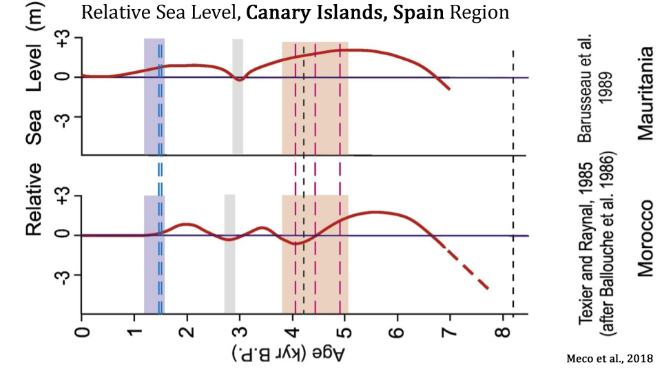
Miguel et al., 2018
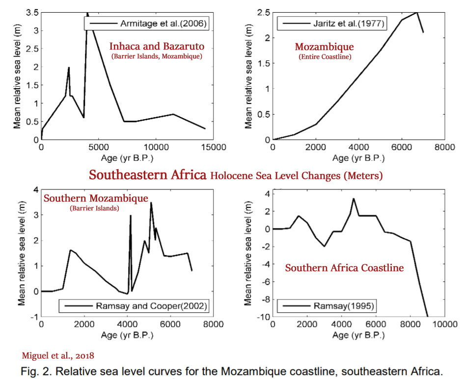
Cooper et al., 2018 With sea level stabilization a few metres above the present around 5.5 ka cal yr BP (Hein et al., 2016), the longshore drift system was reestablished and sediment accumulation in the littoral zone recommenced.
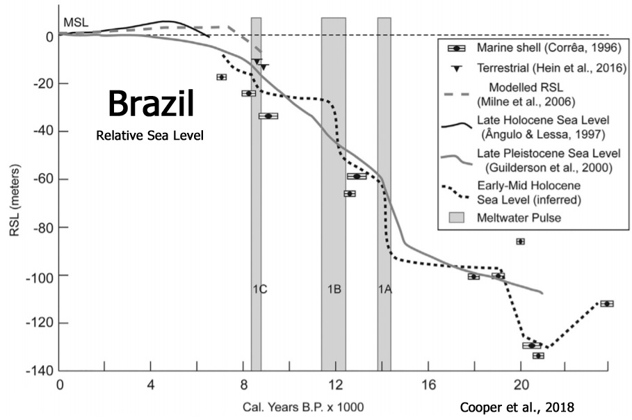
He et al., 2018
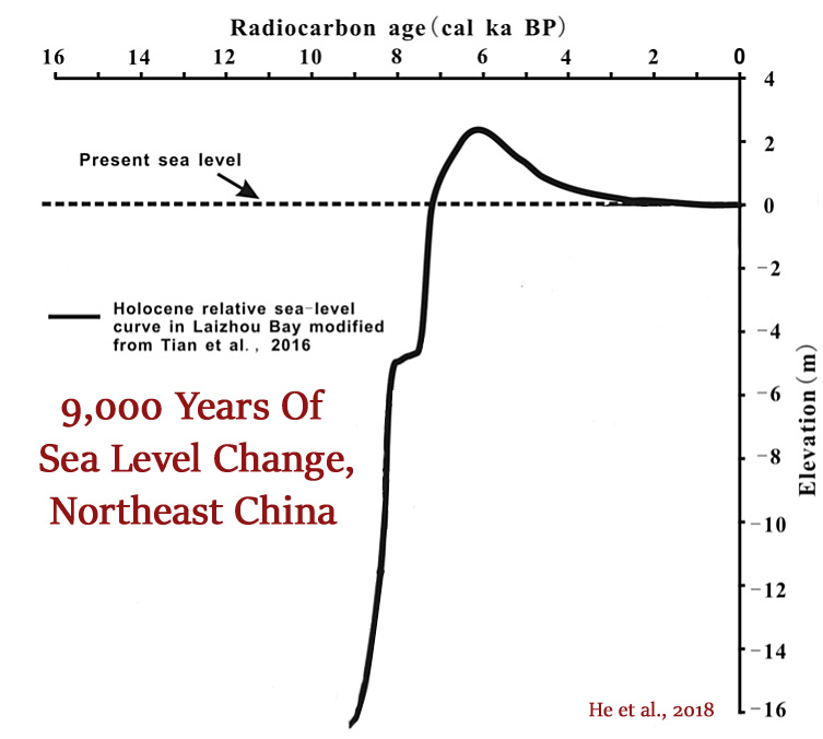
Hallman et al., 2018
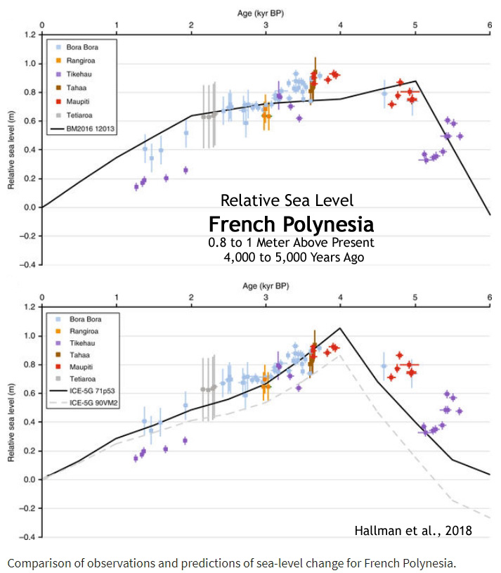
Wündsch et al., 2018 Holocene sea level reconstructions suggest a reduction of the speed of the sea level rise during this time [~7900–6400 cal BP]. The sea level likely reached and exceeded the height of the PSL [present sea level] by as much as 3 m (Compton, 2001).
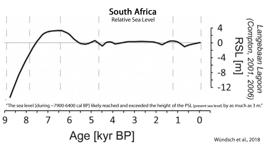
Song et al., 2018 A sea-level curve for the west coast of South Korea was reconstructed. Sea level rose rapidly at a rate of ~1.4 cm yr–1 from 9.8–8.4 cal kyr B.P. [1.4 meters per century] and rose gradually until the mid-Holocene, after which it fell gradually to the present. There is a sea-level highstand of 1–2 m [above present] from 7–4 cal kyr B.P., likely due to hydro-isostatic effects. The rapid sea-level rise during the early Holocene is clearly a manifestation of polar ice sheet decay. The results were supported by the GIA model. The Holocene RSL change on the west coast of South Korea was closely linked to global temperature and ice sheet decay, especially during the early Holocene.
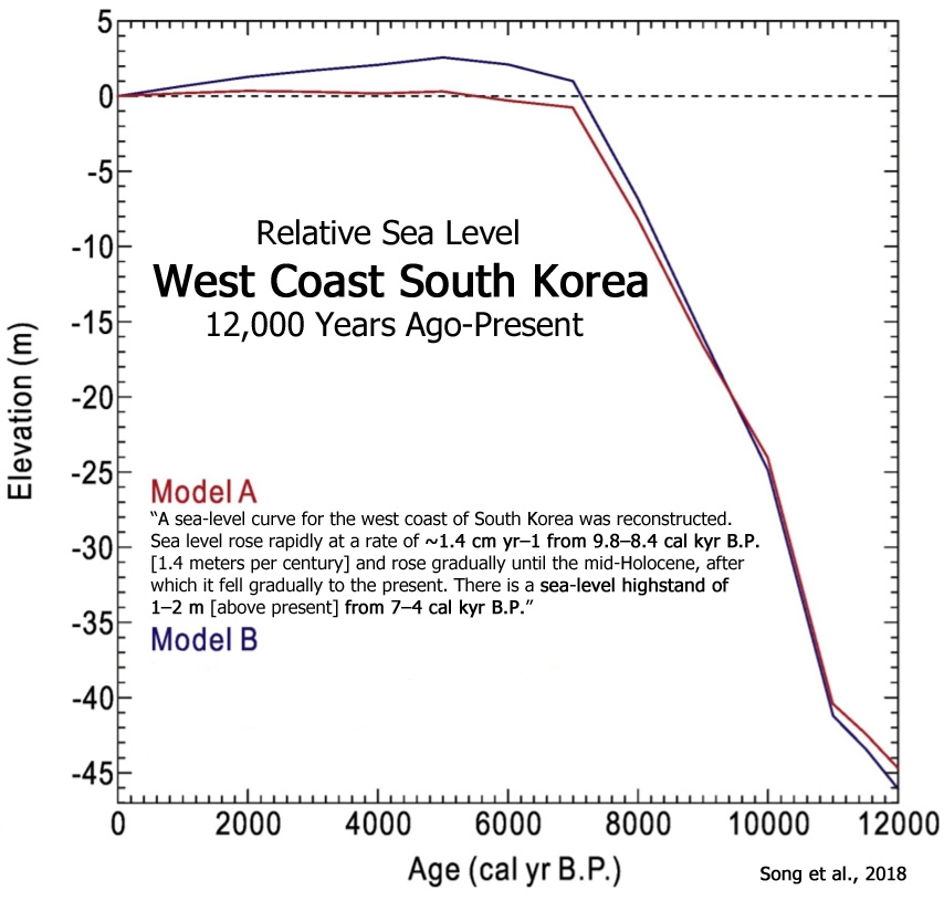
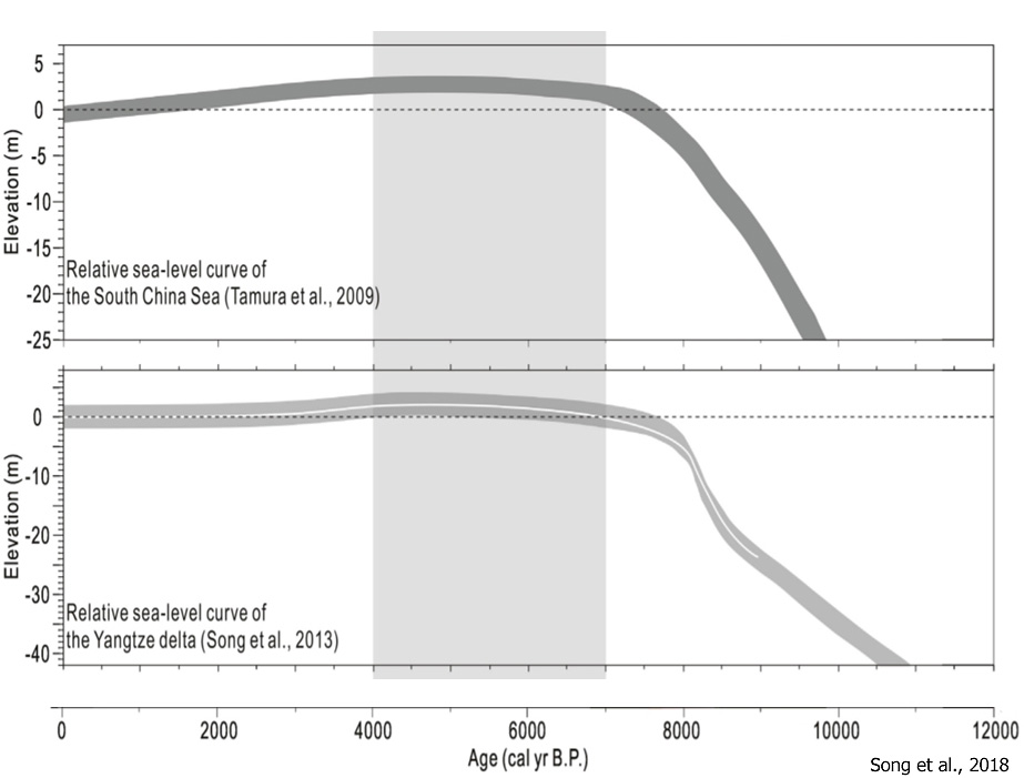
Sloss et al., 2018 A revised Holocene sea-level history for the southern Gulf of Carpentaria [north of Australia] is presented based on new data from the South Wellesley Archipelago and age recalibration of previous research. … By 7700 cal. yr BP, sea-level reached present mean sea-level (PMSL) and continued to rise to an elevation of between 1.5 m and 2 m above PMSL [present mean sea-level]. Sea level remained ca. + 1.5 [meters above present mean sea-level] between 7000 and 4000 cal. yr BP, followed by rapid regression to within ± 0.5 m of PMSL by ca. 3500 cal. yr BP. … A full review of Holocene sea-level around the Australian continental margin is provided by Lewis et al. (2013) which shows that, in general, sea-level around the coastal margin of Australia attained PMSL [present mean sea level] between 8000 and 7400 cal. yr BP, with an elevation of between 1 and 2 m above PMSL [present mean sea level].
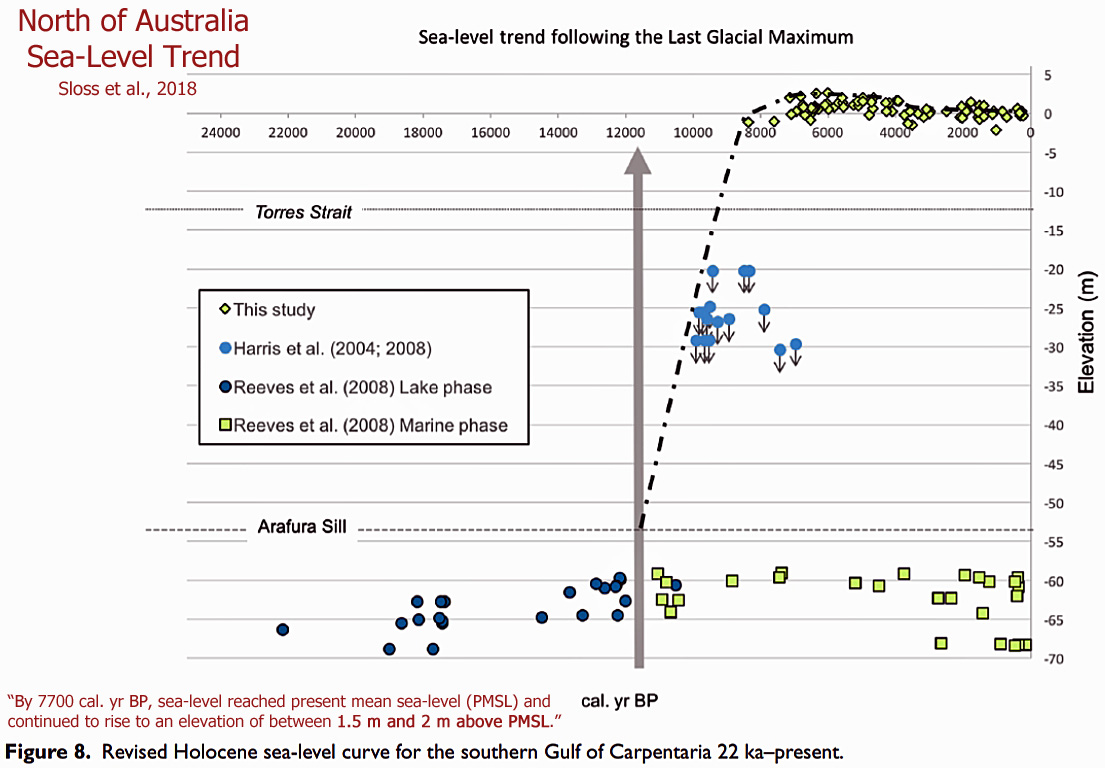
Cooper et al., 2018 Sea-level change around southern Africa (southern Namibia, South Africa, southern Mozambique) since Termination I has been quantified using a variety of indicators. Existing and new data are reviewed to provide a baseline for future studies and identify key research needs and opportunities in the region. While the southern African records broadly agree with other far-field records, detailed Holocene records present as-yet unresolved discrepancies with glacial isostatic adjustment (GIA) model predictions. Two domains, the west coast and east coast are considered. Radiocarbon dated saltmarsh facies and marine shells in life position provide the basis for the west coast sea-level curve back to 9 ka BP. Given the age and elevation uncertainties, a Mid-Holocene highstand of +2 to +4 m [higher than present] is suggested between 7.3 and 6 ka BP, as are several Late Holocene oscillations of <1 m amplitude.
Tam et al., 2018 These sea-level data show that the Holocene sea level in this far-field site has risen rapidly during the early Holocene at a rate averaged around 16.2 ± 4.5 mm/a [+1.6 meters per century] between 10,500 cal a BP at -35.0 ± 4.3 m and 9000 cal a BP at -14.2 ± 1.6 m. The rate of RSL rise was reduced progressively to zero from 9000 to 5000 cal a BP. By the end of this period [5000 cal a BP], the RSL reached a highstand of 3.3 ± 0.2 m [above present]. Since the mid-Holocene, RSL had fallen below-present to -0.60 ± 0.12 m by 800 years ago. This far-field RSL history has been driven by the global ice-volume change that led to the rapid rise in sea level in the early Holocene and by GIA which lifted the RSL for several meters in the mid-Holocene. The gradual fall of RSL during the past 5000 years reflects the diminishing GIA effects and gradual reduction in meltwater input to the oceans.
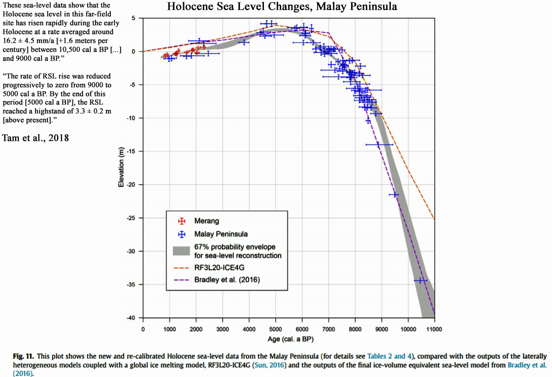
Razjigaeva et al., 2018 The landscape changes during the Medieval Warm Period were discussed for the Kuril and Sakhalin Islands, Primorye and the Amur River Basin. … In all regions, the warming was accompanied by a minor transgression. The sea level was higher than at present by ∼1 m, which resulted in the formation of low marine and lagoon terraces, the attenuation of eolian processes on the coasts, and the fixation of coastal dunes with the development of a thick soil.
Makwana et al., 2018 The enhanced chemical weathering intensities suggest that the last two millennia witnessed two phases of relatively warm and humid climatic conditions, which probably coincide with the Roman Warm Period and the Medieval Warm Period. The Banni Plains was evolved owing to the Middle Holocene high sea stand and subsequent relative fall during the last 2 ka period. The extent of the relative high sea stand up to 2 m above msl also corroborated well by ancient port settlements of the Late Harappan period. … The BB trench site was experiencing a marine environment at least 2.9 ka BP; which hints at a ‘relative sea level’ higher than 2 m from the present msl.
Vacchi et al., 2018 The northwestern portion of Newfoundland differs from the rest of Newfoundland (above ~50 N[…]) and can be classified as uplifting coast. Here, RSL [relative sea level] remained always above the present MSL [mean sea level] in the last ~16 ka. A suite of SLIPs and terrestrial limiting points robustly constrains the RSL evolution in the mid to Late Holocene where RSL dropped from 4.9 ± 3.2 m [above present] at ~5.3 ka to 2.4 ± 2.2 m at ~1.7 ka and finally to the present MSL at ~1.2 ka.
A Model-Defying Cryosphere, Polar Ice
Rösel et al., 2018 We present a continuous time series of in situ measurements from the N‐ICE2015 expedition from January to June 2015 in the Arctic Basin north of Svalbard, comprising snow buoy and ice mass balance buoy data and local and regional data gained from electromagnetic induction (EM) surveys and snow probe measurements from four distinct drifts. The observed mean snow depth of 0.53 m for April to early June [2015] is 73% above the average value of 0.30 m from historical [1955, 1970s] and recent observations in this region, covering the years 1955–2017. The modal total ice and snow thicknesses, of 1.6 and 1.7 m [2015] measured with ground‐based EM and airborne EM measurements in April, May, and June 2015, respectively, lie below the [1970s] values ranging from 1.8 to 2.7 m, reported in historical observations from the same region and time of year [but well above the sea-ice thickness values of 0.94 m for 1955].
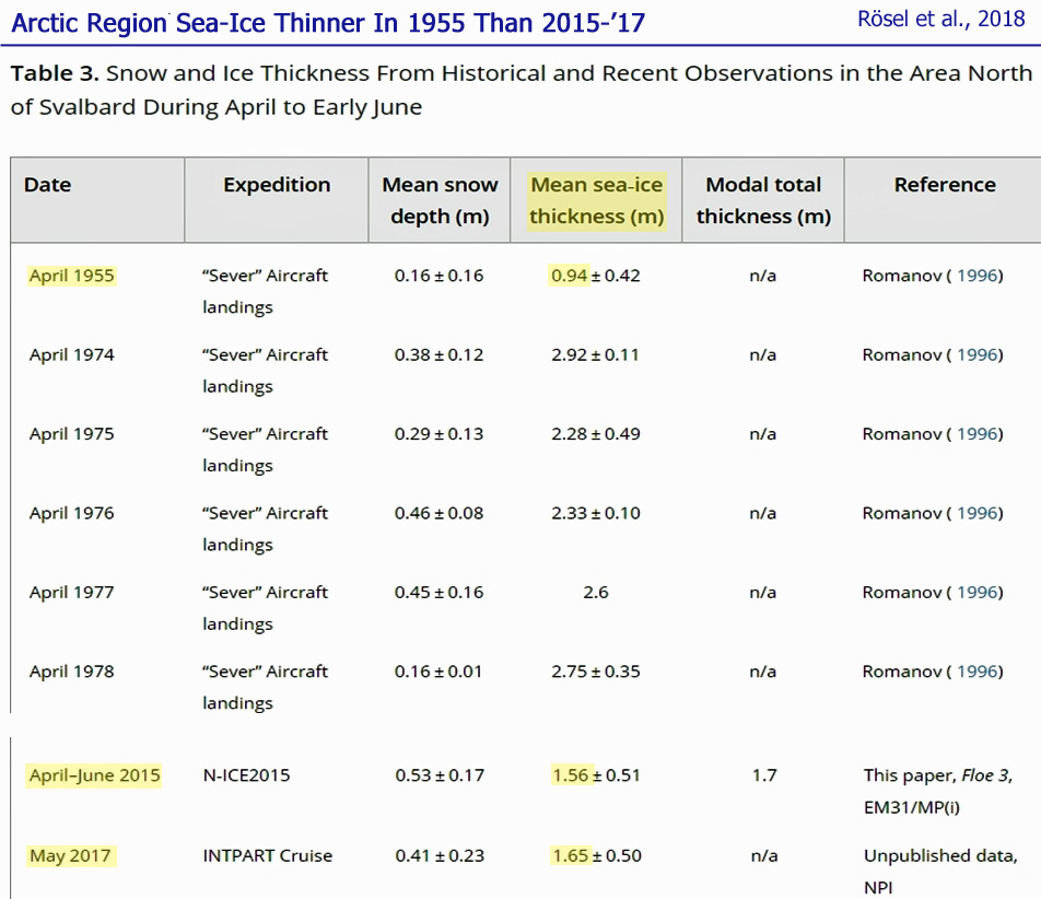
Shakun et al., 2018 Here we show that land-based sectors of the EAIS [East Antarctic Ice Sheet] that drain into the Ross Sea have been stable throughout the past eight million years. … These findings indicate that atmospheric warming during the past eight million years was insufficient to cause widespread or long-lasting meltback of the EAIS [East Antarctic Ice Sheet] margin onto land. We suggest that variations in Antarctic ice volume in response to the range of global temperatures experienced over this period—up to 2–3 degrees Celsius above preindustrial temperatures, corresponding to future scenarios involving carbon dioxide concentrations of between 400 and 500 parts per million—were instead driven mostly by the retreat of marine ice margins, in agreement with the latest models.
Arndt et al., 2018 Pine Island Glacier is the largest current Antarctic contributor to sea level rise. Its ice loss has substantially increased over the last 25 years through thinning, acceleration and grounding line retreat. However, the calving line positions of the stabilizing ice shelf did not show any trend within the observational record (last 70 years) until calving in 2015 led to unprecedented retreat and changed alignment of the calving front. … Despite the thinning and flow acceleration of PIG [Pine Island Glacier], and sustained, rapid thinning of the ice shelf over at least the past 25 years the position of the ice front had not shown any clear trend over 68 years of observations prior to 2015 (Bindschadler, 2002;MacGregor et al., 2012;Rignot, 2002).
Medley et al., 2018 East Antarctic Ice Sheet (EAIS) mass balance is largely driven by snowfall. Recently, increased snowfall in Queen Maud Land led to years of EAIS mass gain. It is difficult to determine whether these years of enhanced snowfall are anomalous or part of a longer-term trend, reducing our ability to assess the mitigating impact of snowfall on sea-level rise. We determine that the recent snowfall increases in western Queen Maud Land (QML) are part of a long-term trend (+5.2±3.7% decade-1) and are unprecedented over the past two millennia. Warming between 1998 and 2016 is significant and rapid (+1.1±0.7 °C decade-1). Using these observations, we determine that the current accumulation and temperature increases in QML from an ensemble of global climate simulations are too low, which suggests that projections of the QML [Queen Maud Land] contribution to sea-level rise are potentially overestimated with a reduced mitigating impact of enhanced snowfall in a warming world.
Treat and Jones, 2018 Rates of permafrost aggradation in peatlands generally increased after 3000 BP and were greatest between 750 and 0 BP [today], corresponding with neoglacial cooling and the Little Ice Age (LIA), respectively.
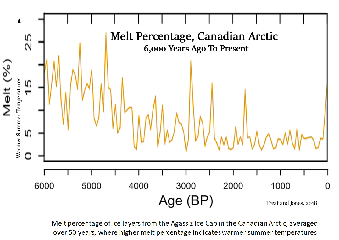
Nature Geoscience, 2018 The East Antarctic ice sheet may be gaining mass in the current, warming climate. The palaeoclimate record shows, however, that it has retreated during previous episodes of prolonged warmth. … In terms of immediate sea-level rise, it is reassuring that it seems to require prolonged periods of lasting hundreds of thousands to millions of years to induce even partial retreat.
Rysgaard et al., 2018 The Greenland ice sheet (GIS) is losing mass at an increasing rate due to surface melt and flow acceleration in outlet glaciers. … Recently it was suggested that there may be a hidden heat source beneath GIS caused by a higher than expected geothermal heat flux (GHF) from the Earth’s interior. Here we present the first direct measurements of GHF from beneath a deep fjord basin in Northeast Greenland. Temperature and salinity time series (2005–2015) in the deep stagnant basin water are used to quantify a GHF of 93 ± 21 mW m−2 which confirm previous indirect estimated values below GIS. A compilation of heat flux recordings from Greenland show the existence of geothermal heat sources beneath GIS and could explain high glacial ice speed areas such as the Northeast Greenland ice stream. … Geothermal springs with source water temperatures above 0 °C have been found all over Greenland, especially around Disko Island in West Greenland, where several thousands of such springs have been identified. … However, the hottest springs, with source water temperatures of 55-62 °C are found in East Greenland at a number of locations north and south of Scoresbysund. … Overall, there has been a gradual warming of the stagnant deep basin bottom water below 240 m depth of 0.017 °C yr−1 from 2005 to 2015. … [T]he gradual temperature increase during 2006–2015 and the spatial distribution of Δθ strongly indicate that bottom water temperatures increase due to a large GHF [geothermal heat flux] in the “Dybet” section. Therefore, we assume that vertical turbulent mixing and GHF [geothermal heat flux] are the primary processes behind the observed salinity and temperature change. … High glacier surface speeds and negative mass balance are also observed near other hot vents in West Greenland such as the Jakobshavn Isbræ (69°N) near Disko Island; [T]he Narssaq bræ, Valhaltinde glacier, Nordbo glacier and Qassimiut ice lobe in South Greenland all show negative ice mass balances near the hot vent in Uunartoq (60°N); [I]n East Greenland the Helheim glacier, Isertoq and Mittivakkat glaciers located near Ikasagitavaq (66°N) are losing mass, and high ice speed is also observed at the Kangerdlugssuaq glacier where a GHF [geothermal heat flux] of 70–80 mW m−2 has been recorded (68°N). In addition, a GHF value of 135 mW m−2 has been reported at NGRIP [North Greenland].
Oppedal et al., 2018 This advance was documented by historical evidence (Hayward, 1983), showing that many glaciers advanced in the twentieth century. Cirque and valley glaciers were at its most advanced position in the 1930s, while larger valley and tidewater glaciers reached their maximum glacier extent in the 1970s. Such a glacier advance is also documented for the Hamberg glacier by Van Der Bilt et al. (2017). Furthermore, during the recession phase after the twentieth century advance, many cirque glaciers deposited annual moraines (Gordon and Timmis, 1992), such as the ones observed in the innermost moraine cluster. Thus, Diamond glacier followed a similar pattern to that observed for small glaciers (0.1–4.0 km2) on South Georgia during the late Holocene, with a Little Ice Age advance, a period of recession, a twentieth century advance and a recent recession (Gordon and Timmis, 1992).
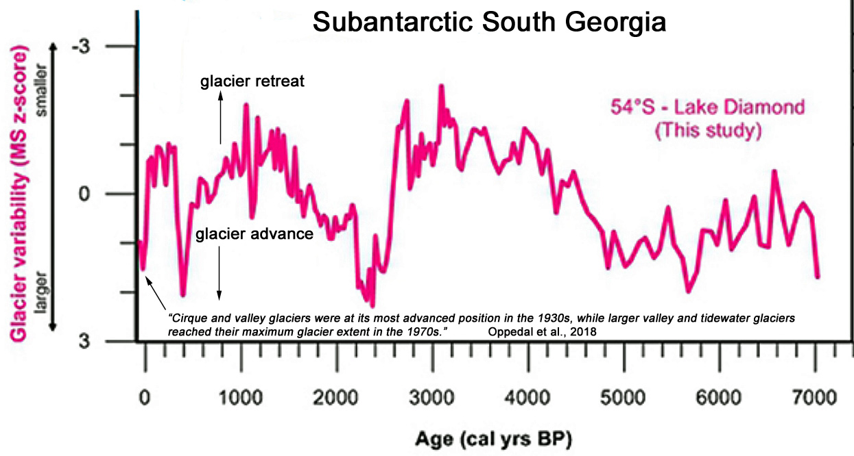
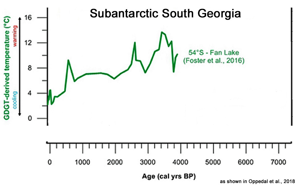
Allan et al., 2018 Our record shows variations with a mean 200 years periodicity until ~2 ka BP, which supports the hypothesis of climate variations driven by solar variability. After 1.5 ka BP, our data show a variability characterized by a 60–70 year periodicity, which suggests linkages with the Atlantic Multidecadal Oscillation and southwestward migration of the atmospheric polar front. The most recent part of the record, from ~1900 CE to 2007 CE, is characterized by assemblages reflecting warmer surface conditions and reduced sea ice cover.
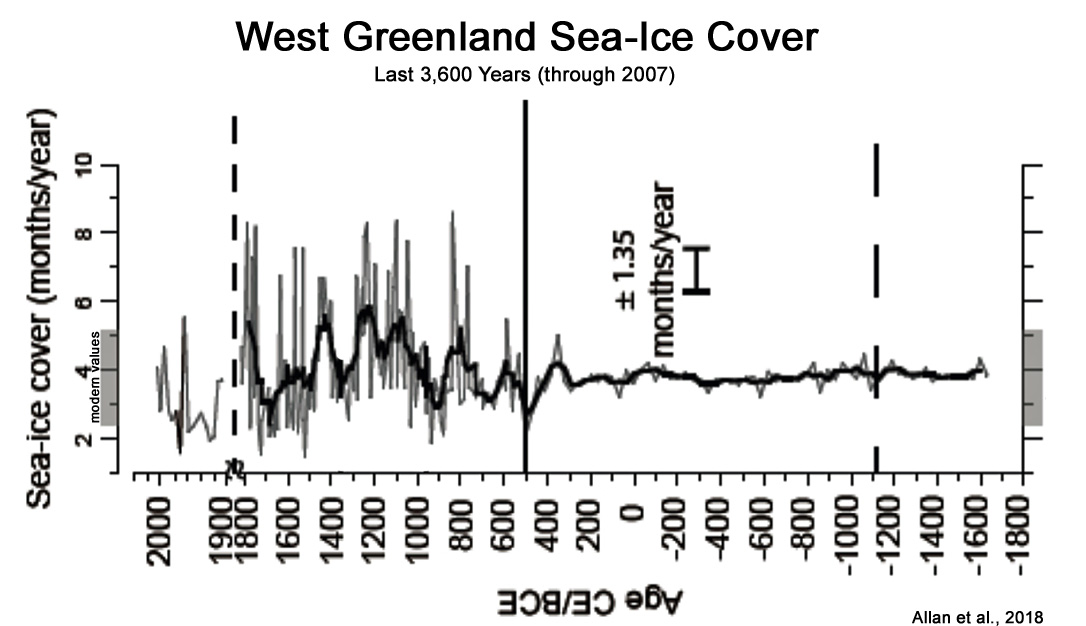
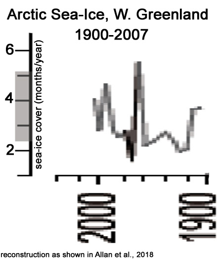
Kelley et al., 2018 In this study, we reconstruct the timing and pattern of middle- and late-Holocene GrIS [Greenland Ice Sheet] margin fluctuations at two locations, ~190 km apart, in central West Greenland using radiocarbon-dated sediment cores from proglacial-threshold lakes. Our results demonstrate that deglaciation occurs at both sites during the early Holocene, with the ice sheet remaining in a smaller-than-present ice margin configuration until ~500 years ago when it readvanced into lake catchments at both sites. … Historical and remote-sensing records indicate that Nordenskiöld Gletscher has been stable or advancing since AD 1950 (Weidick, 1968, 1994). This evidence, in addition to the lack of a moraine or trimline marking the culmination of the late-Holocene advance fronting the ice margin, as occurs across much of the region, infers that the system is at or is still advancing to its late Holocene maximum extent. We note the difference between the ice margin locations on the laterals versus the terminus relative to the late-Holocene maximum position and attribute this to deepening of the glacial trough as described by Kaplan et al. (2009). In fact, observations at the terminus of Nordenskiöld Gletscher in 2013 documented that the terminus is currently advancing onto living tundra.
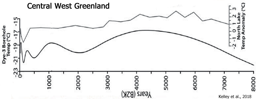
Méheust et al., 2018 In this study, the last glacial–deglacial–Holocene variability in SST [sea surface temperature] and sea-ice cover are reconstructed using alkenone-based SST [sea surface temperature] and sea-ice IP25 and PIP25 proxies in sediment cores from the Bering Sea [Arctic Ocean] and the subarctic Pacific. At all sites and during warm as well as cold climatic intervals SST values are well above 0 °C, suggesting ice-free summer conditions throughout. … The early Holocene is marked by distinctly increased TOC contents, reaching maximum values (>1 wt%) between ~400 and ~170 cm (~11.5–10 ka ~11,500 to 10,000 years ago]). Likewise, continuously increasing SST [sea surface temperature], reaching maximum values of ~ 9°C at ~ 180 cm (~ 10 ka [10,000 years ago]), strongly coincides with the absence of IP25 [proxy for sea ice] in the sediment. … [For the] lower half of the studied section of Core SO202-27-6 [North eastern Pacific], the Holocene is characterized by maximum SST [sea surface temperature] values of 12°C. Relatively low TOC and phytoplankton markers prevailing during this period, coeval with the absence of IP25 [sea ice]. … [For the] North western Pacific (Core SO202 07 6), the Holocene is marked by the absence of IP25 [sea ice], coinciding with low values of TOC, dinosterol and long chain n-alkanes (avg. ~0.5 wt%, ~ 4 µg/g TOC and 78 µg/g TOC, respectively). SST [sea surface temperature] values increase to about 10°C during the early Holocene. … At all sites and during warm as well as cold climatic intervals SST values are well above 0 °C (i.e., ranging between about 5 and 12°C), suggesting that the SST data represent more the summer situation with ice-free conditions.
In the Bering Sea, the transition between the YD [Younger Dryas]-like cold event and the Early Holocene is marked by the rapid disappearance of IP25 [sea ice] around 11.5 ka [11,500 years ago] in both cores from the Bering Sea. The absence of IP25 [sea ice proxy] and minimum PIP25 [sea ice proxy] index values is also registered in the subarctic Pacific during this period. These observations demonstrate that year-round open-water conditions prevailed in these areas during the Early Holocene. … A prominent decrease of IP25 [sea ice proxy] and minimum values of PIP25 index, reflecting ice-free conditions in the subarctic Pacific and the Bering Sea during the Holocene Thermal Maximum, is in line with the SST [sea surface temperature] warming. This is likely due to the maximum orbitally forced summer insolation, enhancing the melting of ice sheets and thus a sea-level rise.
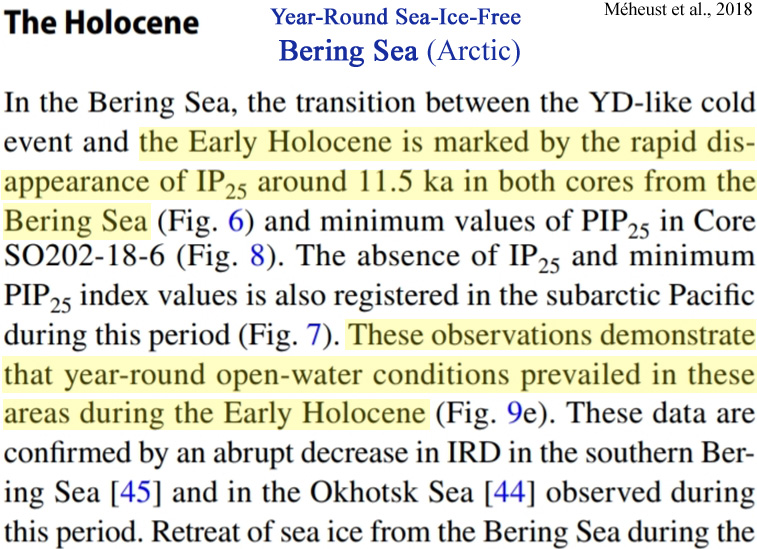
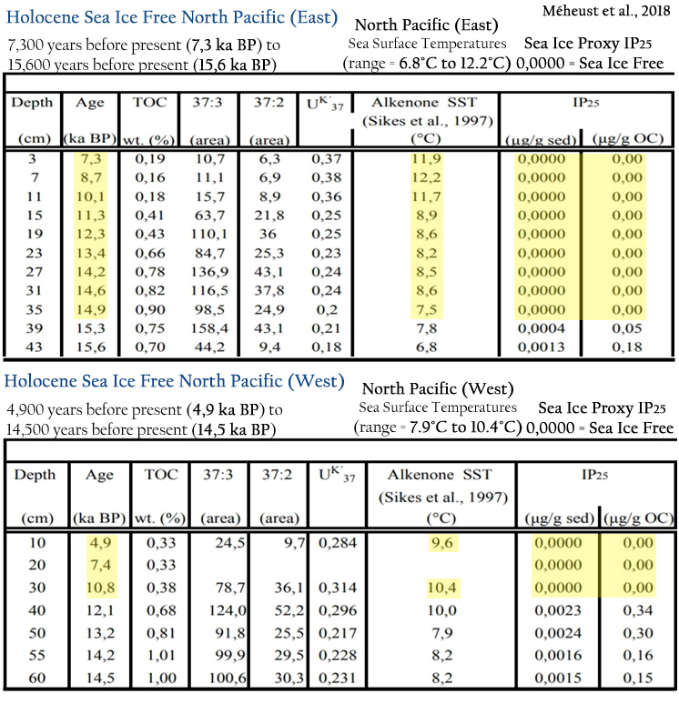
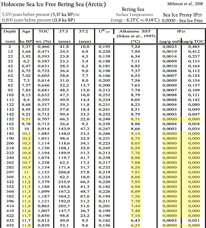
Przybylak et al., 2018 Analysis reveals that the expedition year 1944/1945 in Nordaustlandet was, in the majority of months, the warmest of all analysed periods, that is, both historical and contemporary periods. The study period was markedly warmer than 1981–2010 (mean annual −6.5 vs. −8.4°C) but colder than the periods 2011–2016 (−5.7°C) and 2014–2017 (−5.8°C). … Generally, no change is observed in frequency of occurrence of cold days between the ETCWP [early twentieth century warm period] and CWPs [contemporary warm periods]. A slightly smaller number of cold summer days occurred in the ETCWP than occur at present. … The majority of mean monthly air temperatures in the ETCWP [early twentieth century warm period] is within two SDs of the modern 1981–2010 mean. This means that values of air temperature in the study period [1944/1945] lie within the range of recent temperature variability. Similar results were obtained for older historical periods, for example, for the Canadian Arctic, the entire Svalbard archipelago and surrounding seas, Novaya Zemlya as well as for the entire Arctic.
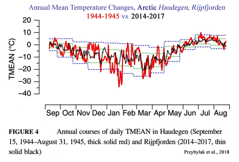
Sigl et al., 2018 No role for industrial black carbon in forcing 19th century glacier retreat in the Alps … Starting around 1860 AD, many glaciers in the European Alps began to retreat from their maximum mid-19th century terminus positions, thereby visualizing the end of the Little Ice Age in Europe. Radiative forcing by increasing deposition of industrial black carbon to snow has been suggested as the main driver of the abrupt glacier retreats in the Alps. … Our study reveals that in 1875 AD, the time when European rBC [industrial black carbon] emission rates started to significantly increase, the majority of Alpine glaciers had already experienced more than 80% of their total 19th century length reduction. Industrial BC emissions can, therefore, not been considered as the primary forcing for the rapid deglaciation at the end of the Little Ice Age in the Alps.
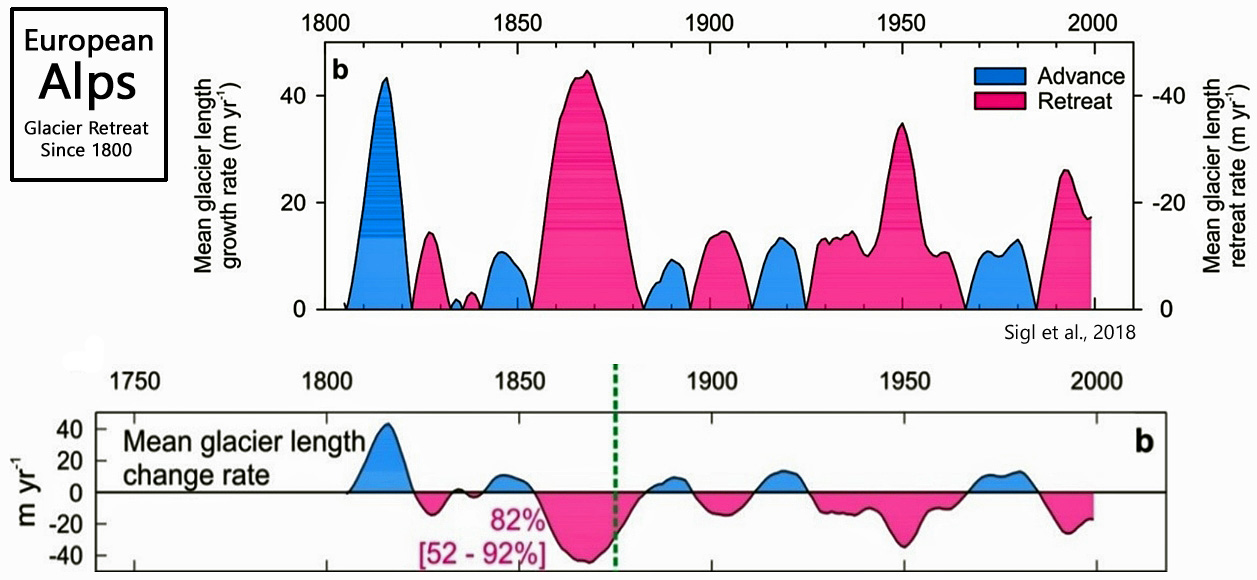
Ronkainen et al., 2018 In our study, we quantify the interannual variability of sea ice thickness in the Bay of Bothnia during the years 2003-2016.
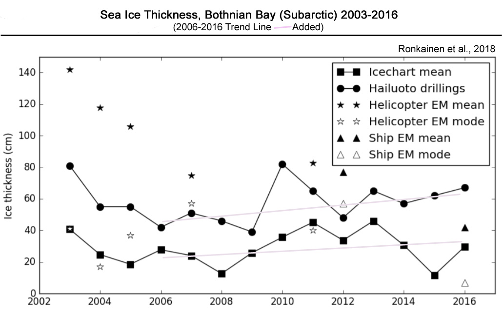
Stabeno et al., 2018 From 2007 to 2013, the southeastern Bering Sea was dominated by extensive sea ice and below-average ocean temperatures. In 2014 there was a shift to reduced sea ice on the southern shelf and above-average ocean temperatures. These conditions continued in 2015 and 2016. … Historically, the dominant parameters controlling sea-ice extent are winds and air temperature, with the persistence of frigid, northerly winds in winter and spring resulting in extensive ice. After mid-March 2014 and 2016 there were no cold northerly or northeasterly winds. Cold northerly winds persisted into mid-April in 2015, but did not result in extensive sea ice south of 58°N. The apparent mechanism that helped limit ice on the southeastern shelf was the strong advection of warm water from the Gulf of Alaska through Unimak Pass. This pattern has been uncommon, occurring in only one other year (2003) in a 37-year record of estimated transport through Unimak Pass. During years with no sea ice on the southern shelf (e.g. 2001–2005, 2014–2016), the depth-averaged temperature there was correlated to the previous summers ocean temperature. … This latest string of three warm years apparently ended this year (2017). In March, sea ice had covered M4, and the ice edge was near or at M2 on 13 March 2017, but by June 2017 the depth-averaged temperatures at M2 were average, indicating that ocean temperature near M2 in 2017 (like the 2006 transition between the previous warm and cold stanzas) will likely be average. With this end of a warm stanza, questions arise. Will the Bering Sea continue in a pattern of warm/cold stanzas?
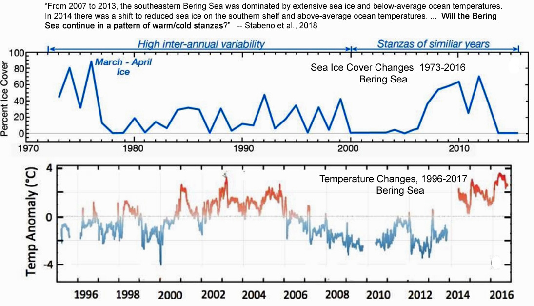
Schannwell et al., 2018 Ice shelf break-up and disintegration events over the past 5 decades have led to speed-up, thinning, and retreat of upstream tributary glaciers and increases to rates of global sea-level rise. The southward progression of these episodes indicates a climatic cause and in turn suggests that the larger Larsen C and George VI ice shelves may undergo a similar collapse in the future. However, the extent to which removal of the Larsen C and George VI ice shelves will affect upstream tributary glaciers and add to global sea levels is unknown. Here we apply numerical ice-sheet models of varying complexity to show that the centennial sea-level commitment of Larsen C embayment glaciers following immediate shelf collapse is low ( < 2.5 mm to 2100, < 4.2 mm to 2300) [0.25 to 0.42 cm added to sea levels by 2100/2300 with Larsen C collapse]. Despite its large size, Larsen C does not provide strong buttressing forces to upstream basins and its collapse does not result in large additional discharge from its tributary glaciers in any of our model scenarios. In contrast, the response of inland glaciers to a collapse of the George VI Ice Shelf may add up to 8mm to global sea levels by 2100 and 22mm by 2300 [0.8 cm to 2.2 cm] due in part to the mechanism of marine ice sheet instability. Our results demonstrate the varying and relative importance to sea level of the large Antarctic Peninsula ice shelves considered to present a risk of collapse.
Barletta et al., 2018 The marine portion of the West Antarctic Ice Sheet (WAIS) in the Amundsen Sea Embayment (ASE) accounts for one-fourth of the cryospheric contribution to global sea-level rise and is vulnerable to catastrophic collapse. The bedrock response to ice mass loss, glacial isostatic adjustment (GIA), was thought to occur on a time scale of 10,000 years. We used new GPS measurements, which show a rapid (41 millimeters per year) uplift of the ASE, to estimate the viscosity of the mantle underneath. We found a much lower viscosity (4 × 10¹⁸ pascal-second) than global average, and this shortens the GIA response time scale to decades up to a century. Our finding requires an upward revision of ice mass loss from gravity data of 10% and increases the potential stability of the WAIS against catastrophic collapse. … This means that as ice is lost, the crust rebounds much faster than previously expected. Although estimates of total ice loss have to be revised upward, the surprising finding indicates that the ice sheet may stabilize against catastrophic collapse.
Lv et al., 2018 Here, we utilize Landsat 7, Landsat 8, and ASTER optical images acquired between 1999 and 2016 to characterise the dynamics of the glaciers in the Kingata Mountains, located in the eastern Pamir. We quantify the velocity, areal, and frontal changes of these glaciers, which provide us with valuable data on their recent dynamic evolution and an indication of how they may evolve in future years. We highlight 28 glaciers among which 17 have changed markedly over the study period. We identify 4 advancing glaciers, 1 receding glacier, and 12 surge-type glaciers. The dynamic evolution of the glacier surges shows some similarity with those of the nearby Karakoram, suggesting that both hydrological and thermal controls are important for surge initiation and recession.
Kolling et al., 2018 Our biomarker record indicates that Disko Bugt [West Greenland] experienced a gradual expansion of seasonal sea ice during the last 2.2 kyr. Maximum sea ice extent was reached during the Little Ice Age around 0.2 kyr BP. Superimposed on this longer term trend, we find short-term oscillations in open water primary production and terrigenous input, which may be related to the Atlantic Multidecadal Oscillation and solar activity changes as potential climatic trigger mechanisms. … The period between 2.2 and 1.2 kyr BP, with lower than modern sea ice conditions in Disko Bugt (Fig. 6b), coincides with generally warm conditions over the Greenland Ice Sheet. … During the last 0.1 kyr, all biomarker concentrations showed an increase, brassicasterol and HBI III reach maximum values in the uppermost sample (80 µg/gTOC and 1.8 µg/gTOC, respectively; Fig. 3b, d). … [During the Little Ice Age (0.7–0.2 kyr BP)] our biomarker record supports harsher sea ice conditions, possibly similar to conditions as observed today (Fig. 6b), indicated by strong increased in IP25 concentration and the PDIP25 index (Fig. 4c, d). … A self-amplifying system may have caused the environmental changes observed in Disko Bugt area as follows: solar triggered Arctic sea ice melt [Ruzmaikin et al., 2004] increases freshwater supply towards the North Atlantic causing a reduction in sub-polar gyre activity and AMO [Holland et al., 2001, Schmith et al., 2003] as described by Sha et al. [2016]. This may in turn cause distinct changes in WGC composition and meltwater supply from the Greenland Ice Sheet that affects phytoplankton blooms in West Greenland. … We find that the Disko Bugt area was influenced by seasonal sea ice over the last 2.2 kyr BP. The overall sea ice trend indicates a development from a reduced sea ice cover during early spring, with sea ice algae productivity hampered by light availability to a gradual extend of the sea ice season from 1.2 kyr BP onwards. This change in sea ice extend is parallel to decreasing Northern Hemisphere atmospheric temperatures and culminates in the Little Ice Age around 0.2 kyr. We assume that modern conditions, with sea ice present until late spring and the presence of a stable ice edge at Disko Bugt, established around that time [~200 years ago].
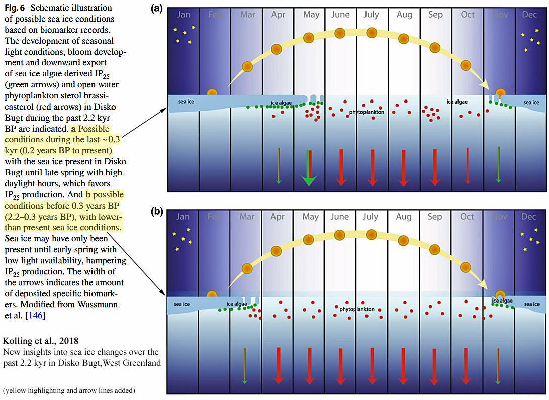
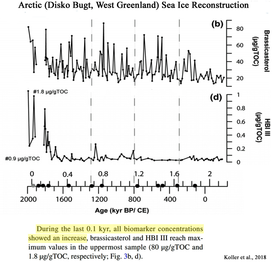
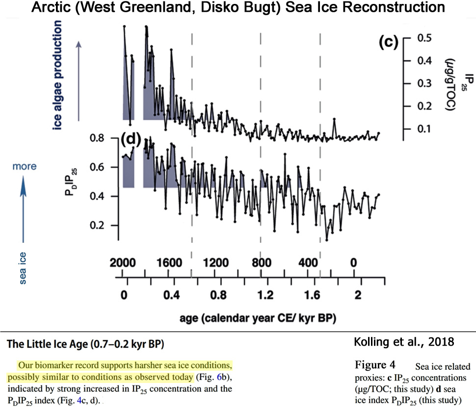
An et al., 2018 A Century of Stability of Avannarleq and Kujalleq Glaciers, West Greenland … We digitize the summer ice front positions using aerial photos from 1964 (Carbonnell & Bauer, 1968) and Landsat imagery spanning 1976 to 2017. AVA did not retreat at a significant level (150–200 m) during the entire time period (Figure 1). KUJ advanced and retreated over a region about 2.5 km wide. At midrange in the 1960s to 1970s, the ice front advanced in the 1980s, remained at an advanced position in the 1990s, and retreated by 1.5 km from 1997 to 2001. The ice front of KUJ has remained stable within ±300 m since 2001. On the longer term, AVA has not migrated more than 100 m since 1903, while KUJ retreated by 2 km in 1851–1949, followed by stable conditions in 1949–1961, and a readvance of 700 m in 1961–1964 (Weidick, 1968). … High-resolution airborne gravity acquired at a low aircraft speed, with low ground clearance, combined with novel multibeam echo sounding data of the fjord helps resolve the bed topography and ice thickness of major outlet glaciers flowing into the ice-chocked Torssukatak Fjord in central West Greenland. The results explain the exceptional stability of two large glaciers over the last 1.5 century, despite the presence of warmer ocean waters in the fjord since the mid-1990s, because the glaciers are protected from the ocean by sills at the end of deep (700 m) fjords. The retreat of these glaciers from the deep fjords to the sills precedes year 1851.
Tong et al., 2018 Glaciers and ice streams drain the ice from the ice sheets to the ice shelves, and contribute to global sea-level changes. Therefore, ice velocity is an essential parameter for the assessment of mass balance. … The results show that the estimated velocity obtained by the use of the proposed method is superior to the other methods, and the long-term series of ice velocity measurements shows that the ice velocity in the Amery Ice Shelf has hardly changed over the past 45 years (1968–2014). We conclude that the ice flow velocity of the Amery Ice Shelf has showed a slight deceleration over the past 45 years.
Hörner et al., 2018 IP25 concentrations and PIP25 values are low (less IP25 biomarkers and increased phytoplankton biomarkers) between 11 and 8 ka (Core BP00-36/4; Fig. 7c) reflecting less sea ice cover in the central Kara Sea after the cold interval. This warmer phase designated as the Holocene Thermal Maximum (HTM), was caused by the insolation maximum in the Northern Hemisphere (e.g., Koç et al. [93]; Bauch et al. [22]; Hald et al. [94]; Risebrobakken et al. [95]; Fig. 7c). The warmer climate was also documented in other parts of the high latitudes by reduced sea ice cover in the eastern and western Laptev Sea [54, 96] and by warmer and moister climate in the Siberian hinterland [97, 98]. Moreover, warmest atmospheric temperatures were recorded in Greenland ice cores during this interval [92, 99].
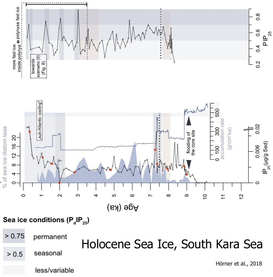
Engel et al., 2018 Two small glaciers on James Ross Island, the north-eastern Antarctic Peninsula, experienced surface mass gain between 2009 and 2015 as revealed by field measurements. A positive cumulative surface mass balance of 0.57 ± 0.67 and 0.11 ± 0.37 m w.e. was observed during the 2009–2015 period on Whisky Glacier and Davies Dome, respectively. … Ambrožová and Láska (2016) reported a significant decrease (0.03–0.15°C a−1 [-0.3 to -1.5°C per decade]) in the temperature along the AP [Antarctic Peninsula] over the 2005–15 period with the most prominent cooling at the Bibby Hill station on JRI [James Ross Island]. … The cumulative mass gain of the glaciers around the northern AP [Antarctic Peninsula] indicates a regional change from a predominantly negative surface mass balance in the first decade of the 21st century to a positive balance over the 2009–15 period. The change in the glacier mass balance follows a significant decrease in the warming rates reported from the northern AP [Antarctic Peninsula] since the end of the 20th century. The mass gain is also consistent with the regional trend of climate cooling on the eastern side of the AP [Antarctic Peninsula].
Lemos et al., 2018 We have presented a new, high temporal resolution record of ice velocity evolution for four important, high discharge marine-based glaciers in Greenland, updated to the present day (October 2014 to February 2017). … At J1 […], the average seasonal variability in ice speed was 400 m yr−1 during 2009–2011, increasing by more than a factor of 3, to 1400 m yr−1 between 2012 and 2013 and then diminishing to 750 m yr−1 between 2015 and 2017. Turning to the longer term evolution of JI (Fig. 5; time series location shown in Fig. 1), fitting a linear trend to the data suggests an annual acceleration since 2009 of ∼ 218 m yr−1 at Jif, diminishing inland to ∼ 128 m yr−2 at J1, and ∼ 102 m yr−2 at J2. Although this provides a simple characterization of the longer-term evolution in ice speed, it is clear from our time series that computing a linear trend does not capture the full decadal-scale variability in ice velocity. In particular, we note that much of the acceleration occurred between 2011 and 2013 (Fig. 5b and c), and since then there has been a notable absence of multi-annual acceleration as earlier records suggest (Joughin et al., 2014). Computing trends in ice velocity since 2012 near the glacier terminus (Jif), for example, shows a modest decline in speed of 321 m yr−2 over the 5-year period (Fig. 5b). The calving front position migration has been suggested as the trigger to the stresses regimes variations and consequently the main driver to the JI velocity fluctuations (Joughin et al., 2008a, b, 2012, 2014; Bondzio et al., 2017). After a successive and gradually increased rate of ice front retreat until 2012 (Fig. 5a), the JI grounding line is now located on a higher bed location (Joughin et al., 2012; An et al., 2017). This may be acting to stabilize the grounding line, and in turn contribute to the glacier deceleration, although the main cause remains to be determined and further investigations is necessary.
Yu and Zhong, 2018 The underlying physical mechanisms for the Arctic warming and accelerated sea ice retreat are not fully understood. In this study, we apply a relatively novel statistical method called Self-Organizing Maps (SOM) to examine the trend and variability of autumn Arctic sea ice in the past three decades and their relationships to large-scale atmospheric circulation changes. Our results show that the anomalous autumn the Arctic Dipole (AD) (Node 1) and the Arctic Oscillation (AO) (Node 9) could explain in a statistical sense as much as 50% of autumn sea ice decline between 1979 and 2016. The Arctic atmospheric circulation anomalies associated with anomalous sea surface temperature patterns over the North Pacific and North Atlantic influence Arctic sea ice primarily through anomalous temperature and water vapour advection and associated radiative feedback. … We investigate the potential mechanisms for the autumn arctic sea ice decline for the period 1979-2016 using the SOM method. Our results show that more than half of the autumn Arctic sea ice loss may be associated with the changes in the temperature and water vapour transport and the associated water vapour radiation feedback resulting from anomalous atmospheric circulations linked to SST anomalies over the North Pacific and North Atlantic. … [T]he results here help advance the knowledge about the relatively large contributions from the decadal-scale natural climate variability to Arctic climate change, though further studies using coupled global atmosphere-ocean-sea ice models are warranted to fully understand the physical mechanisms.
Belt, 2018 Exceptionally, Massé et al. (2011) observed a general decline in sedimentary IPSO25 concentration in a short offshore transect from East Antarctica; a trend shown subsequently to be quite general for various other Antarctic regions (Belt et al., 2016). In the latter study, it was suggested that the origin of this trend might be found in the preferred habitat of the known source of IPSO25 (B. adeliensis), which has a tendency to proliferate in platelet ice, found most commonly in near-shore locations covered by fast ice (Medlin, 1990). As such, it was hypothesised that higher concentrations of IPSO25 might be found in locations proximal to ice shelves, since their basal melt acts as the major driver for platelet ice formation (Jefferies et al., 1993). Re-examination of some palaeo sea ice records based on IPSO25 added further credibility to this suggestion (Fig. 6), and Smik et al. (2016a) also identified highest concentrations of IPSO25 in near-shore surface waters soon after spring sea ice melt.
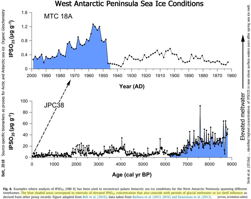
Bjørk et al., 2018 Here, we present the first record of direct Holocene ice-marginal changes of the Helheim Glacier following the initial deglaciation. By analysing cores from lakes adjacent to the present ice margin, we pinpoint periods of advance and retreat. We target threshold lakes, which receive glacial meltwater only when the margin is at an advanced position, similar to the present. We show that, during the period from 10.5 to 9.6 cal ka BP, the extent of Helheim Glacier was similar to that of today’s, after which it remained retracted for most of the Holocene until a re-advance caused it to reach its present extent at c. 0.3 cal ka BP, during the Little Ice Age (LIA). [The glacier’s present extent is not different than it was 300 years ago, during the Little ice Age.] Thus, Helheim Glacier’s present extent is the largest since the last deglaciation, and its Holocene history shows that it is capable of recovering after several millennia of warming and retreat. Furthermore, the absence of advances beyond the present-day position during for example the 9.3 and 8.2 ka cold events as well as the early-Neoglacial suggest a substantial retreat during most of the Holocene. … Our results show that the ice sheet significantly retreated during the HTM [Holocene Thermal Maximum] 8-5 ka BP when temperatures were 2-4°C warmer than now (Axford et al., 2013; Buizert et al., 2018). Reconstructed summer temperatures from central east Greenland show also a pronounced early Holocene warming (Axford et al., 2017). Therefore, we infer significant retreat during the HTM since the increasing cold conditions commencing at c. 5 cal. ka BP were not sufficient to advance the glacier margin to its present position.
Köseoğlu et al., 2018 The core 70 site is characterised by extensive modern sea ice conditions (≈80% SpSIC [Spring Sea Ice Concentration]) and the downcore record represents a gradual evolution of sea ice cover in the northern Barents Sea from ice-free conditions during the early Holocene to prolonged seasonal sea ice presence prevalent in the region today. The primarily insolation-controlled southward expansion of sea ice cover previously inferred for the core site throughout the Holocene (Belt et al., 2015; Berben et al., 2017) is reflected in the CT model assessment. Consistent with the onset of the Holocene Thermal Maximum and the resulting proximity of the annual maximum sea ice edge to the core site between ca. 9.5–8.5 cal kyr BP evident from low PIIIIP25-derived SpSIC (ca. 5–15%), the CT model predicts mostly marginal sea ice conditions during this interval. … From ca. 10.0–1.5 cal kyr BP, ice-free conditions characterised the core 11 site, as evidenced by consistently low SpSIC (ca. <10%) and marginal sea ice conditions predicted by the CT model, and further supported by an enhancement of AW [Arctic Water] inflow to the core site from ca. 9.8 cal kyr BP (Groot et al., 2014).
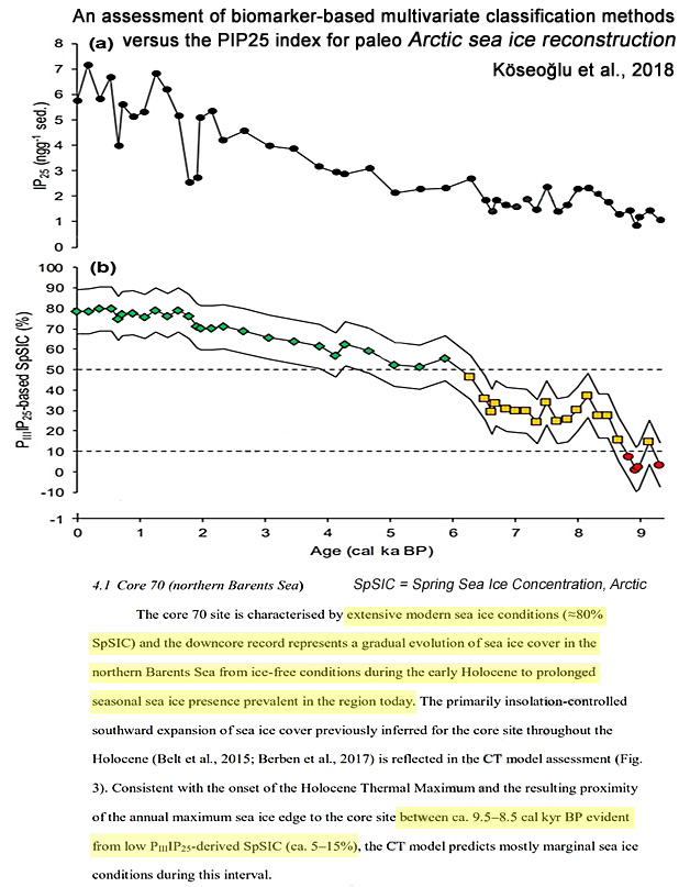
Lovell et al., 2018 Most large tidewater glaciers in Svalbard are known to have surged at least once in the last few hundred years. However, very little information exists on the frequency, timing or magnitude of surges prior to the Little Ice Age (LIA) maximum in ∼1900. We investigate the sediment-landform assemblages produced by multiple advances of the Nathorstbreen glacier system (NGS) in order to reconstruct its Late Holocene surge history. The glacier has recently undergone one of the largest surges ever observed in Svalbard, advancing ∼16 km from 2008 to 2016. … By combining these data with previous marine geological investigations in inner and outer Van Keulenfjorden, we demonstrate that NGS [Nathorstbreen glacier system] has advanced at least four times prior to the recent 2008–2016 surge: twice at ∼2.7 kyr BP, at ∼1160 AD, and in ∼1890. This represents a unique record of the timing and magnitude of Late Holocene tidewater glacier surges in Svalbard.
Fjeldskaar et al., 2018 About 60% of Svalbard is covered by glaciers today, but many of these glaciers were much reduced in size or gone in the Early Holocene. High resolution modeling of the glacial isostatic rebound reveals that the largest glaciers in Nordaustlandet and eastern Spitsbergen survived the Early Holocene warming, while the smaller, more peripheral glaciers, especially in the northwest, started to form about 5,500 years ago, and reached 3/4 of their current size about 600 years ago. Relative sea level has been rising during the last few millennia in the north and western parts of Spitsbergen, while land still emerges in the remaining part of Svalbard. Here we show that this sea level rise in the northwest is caused by the regrowth of glaciers in the Mid- to Late Holocene that slowed down, and even reversed, the post-glacial isostatic uplift and caused the crust to subside over large areas of Spitsbergen.
Røthe et al., 2018 Reconstructing Holocene Glacier and Climate Fluctuations From Lake Sediments in Vårfluesjøen, Northern Spitsbergen … Here, we present work from the northern coast of Spitsbergen in which we unravel the sediment sequence from a distal glacier-fed lake, Vårfluesjøen. … During the early Holocene, the glaciers in the Vårfluesjøen catchment were considerably smaller than today or had even melted completely. … D’Andrea et al. (2012) […] point to increased heat transport via the West Spitsbergen Current, and accompanying increased winter precipitation, rather than cold temperatures, to have caused LIA expansions on Svalbard. … During the early and mid-Holocene period, other glacier reconstructions from the west coast of Svalbard suggests that many glaciers were small or completely melted during this time interval (Svendsen and Mangerud, 1997; Røthe et al., 2015; van der Bilt et al., 2015; de Wet et al., 2018). Mangerud and Svendsen (2018) postulated that August temperatures in Svalbard were 6°C warmer from 10000 to 9000 cal. yr. BP than they are today, based on the presence of Zirfaea crispate.
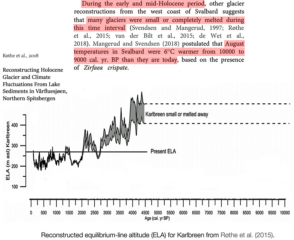
Ding et al., 2018 This simulated internal variability shows a strong similarity to the observed Arctic atmospheric change in the past 37 years. Through a fingerprint pattern matching method, we estimate that this internal variability contributes to about 40–50% of observed multi-decadal decline in Arctic sea ice. Our study also suggests that global climate models may not actually underestimate sea ice sensitivities in the Arctic, but have trouble fully replicating an observed linkage between the Arctic and lower latitudes in recent decades. Further improvements in simulating the observed Arctic–global linkage are thus necessary before the Arctic’s sensitivity to global warming in models can be quantified with confidence. … Our analysis indicates that the discrepancy between observed and simulated sea ice trends can be reconciled in large part by recognizing that internal variability may have been as important as anthropogenic influences on Arctic sea ice decline over the past decades. This result conflicts with previous studies.… [A]s much as 30% of global surface air temperature change may be in response to sea ice loss rather than being driven by it.
McKay et al., 2018 In total, observations from 144 sites north of 57°N that span at least the interval from 6 to 2 ka, and that had median Holocene temporal resolution of <500 yr were included in the analysis. … Across all observations (Fig. 2a), the area-weighted total distribution of cooling onset ages indicates two primary intervals of when cooling began or accelerated. The first, beginning ca. 7 ka, primarily captures cooling following peak summer warm conditions in the early- to mid-Holocene, when nearly all Arctic glaciers were smaller than during 20th century positions. … The first-order structure of Holocene glaciation in the Arctic is a general increase in the size of glaciers from the early Holocene through the Little Ice Age (Fig. 3). From 8-6.5 ka, glaciers were uniformly retreated or absent throughout the Arctic.
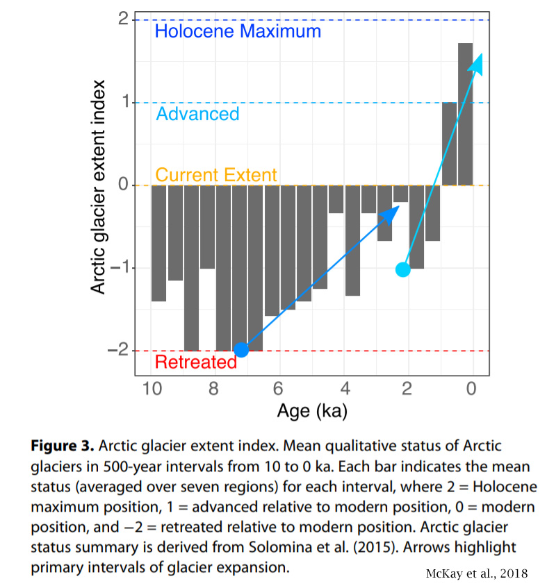
Jena et al., 2018 In the backdrop of global warming, Antarctic sea-ice variability showed an ovhttps://notrickszone.com/wp-content/uploads/2019/06/Arctic-glacers-during-the-Holocene-McKay-2018.jpgerall expansion with the regional heterogeneity of increasing and decreasing patterns. Analysis of satellite derived sea-ice extent, during 1979 to 2015, in the Indian Ocean sector of Antarctica (IOA) revealed expansion of 2.4±1.2% decade-1. We find strengthening of westerly wind during the austral summer (between 50°S to 62°S) facilitated northward advection of a cool and fresh layer.
Mass Extinction Events Caused By Global Cooling, Glaciation, Sea Level Fall
Isozaki and Servais, 2018 Besides the similarity in extinction patterns with the preferential elimination of particular clades, we can recognize a major resemblance but of non-biotic nature between the [Ordovician] Hirnantian and [Permian] Capitanian [mass extinction] events, that is the significant cooling coupled with global sea-level drop. … A sea-level drop of nearly 100 m can be achieved solely by transferring vast seawater onto land in the form of ice. It is noteworthy that sea level was much higher in the Late Ordovician (ca. 60 m above the present-day level) than in the Middle Permian (ca. 80 m below the present-day level), even after the sea-level drop in the same magnitude. … The lines of evidence for cooling and relevant sealevel drop during the Hirnantian [Ordovician] are listed as follows: (1) sequence stratigraphy (Haq & Schutter 2008; Fig. 2); (2) regional occurrence of glacial sediments, including tillite/dropstone, mostly in Gondwana (e.g. Brenchley et al. 1994; Ghienne 2003); and (3) isotope signature in seawater (Trotter et al. 2008). On the basis of these, there was a solid consensus among researchers for the link between the global cooling and the first Hirnantian extinction; however, recent studies indicate that the cooling may have started not necessarily at the beginning of the Hirnantian but much earlier, probably already in the Middle Ordovician (Vandenbroucke et al. 2010; Finnegan et al. 2011; Nardin et al. 2011; Rasmussen et al. 2016). Nevertheless, sea level dropped nearly 100 m in the Hirnantian (e.g. Haq & Schutter 2008). Traditionally, the existence of a continental block (Gondwana) over the South Pole was required for the development of ice sheets. … The evidence for the late Capitanian global sealevel drop (for up to 100 m) is robust. … The sharp erosion of reef limestone in low-latitude mid-ocean implies a large eustatic sea-level drop, in other words, the appearance of a global cooling. … The biotic responses in the Hirnantian and Capitanian appear compliant with all these lines of evidence for cooling, in particular, the latitudinal contraction of faunal distributions towards tropics together with the preferential elimination of preexisting tropical fauna. Regardless of the second Hirnantian episode, the first decline in biodiversity in both cases occurred during global cooling. In general, a relative drop in seawater temperature, particularly in shallow seas, is critical for the metabolism of almost all contemporary marine organisms. The updated lines of evidence therefore confirmed the classic notion of a putative link between the global cooling and extinction (e.g. Stanley 1988) for both cases [the Ordovician and Permian extinction events].
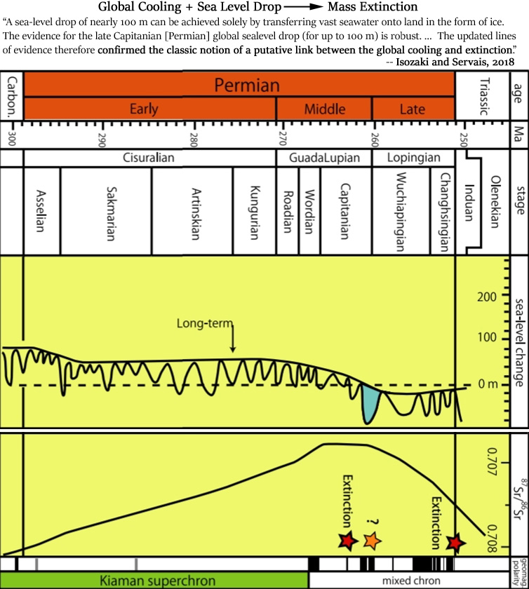
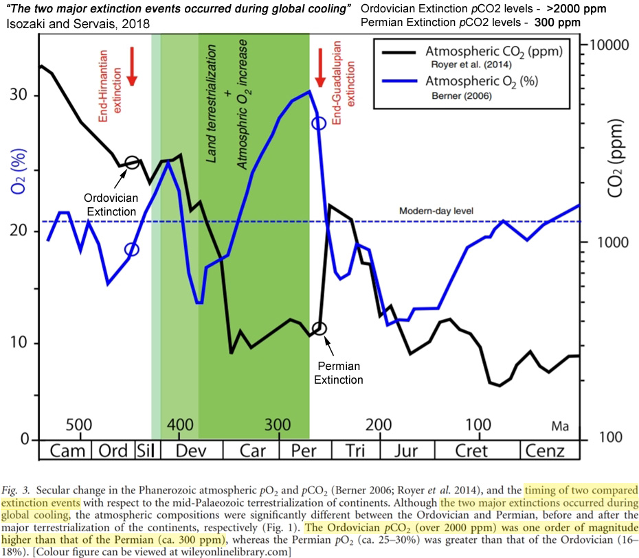
Kani et al., 2018 The end-Middle Permian extinction was in fact a prolonged but gradual decrease in diversity from the Wordian to the end of the Capitanian (Clapham et al., 2009). The main phase of the extinction appears to have occurred almost simultaneously during the Capitanian minimum of Sr isotope records. … [T]he sea level during the Capitanian contradictorily recorded the lowest stand of the Phanerozoic (Haq and Schutter, 2008), suggesting a global cooling instead [caused the Permian extinction]. Ice coverage and/or the predominance of arid climates under cooling during the Permian likely accelerated the decrease in the seawater Sr ratio. … In general, the termination of shallow marine carbonates may occur with a decrease in the seawater temperature. Two possible causes can be inferred for the late Capitanian temperature decrease, i.e., 1) the appearance of global cooling, and 2) the migration of depositional sites to higher latitudes with cooler climates. The Capitanian global cooling was proposed first on the basis of the unique carbon isotope record in low-latitude paleo-atoll carbonates (12°S) (Isozaki et al., 2007), a signature that was reproduced later in other parts of the world, e.g., in Croatia and in South China (Isozaki et al., 2011; Chen and Benton, 2012). In addition, in a global summary of sequence stratigraphy (Haq and Schutter, 2008), the findings of coeval glacial deposits in eastern Australia and in Mongolia (Fielding et al., 2008; Fujimoto et al., 2012), the selective extinction of tropical fauna (Isozaki and Aljinovic, 2009), the migration of mid-latitude fauna to low latitudes (Shen and Shi, 2002), and the Milankovitch tuning (Fang et al., 2017), all support the onset of cooling in the Capitanian. … [T]he Capitanian under a cooling trend […] [coincided with the] lowest sea level of the Phanerozoic and […] the preferential elimination of tropical fauna. … [T]he appearance of extensive ice coverage over continental blocks might have occurred, and the weathering/erosion of continental crust could have been suppressed to drive a lower riverine flux with high 87Sr/86Sr ratios. Alternatively, an arid weathering regime might have developed extensively under the cool climate, particularly on the vast supercontinent Pangea, which also contributed to suppressing the riverine fluxes (Korte et al., 2006).
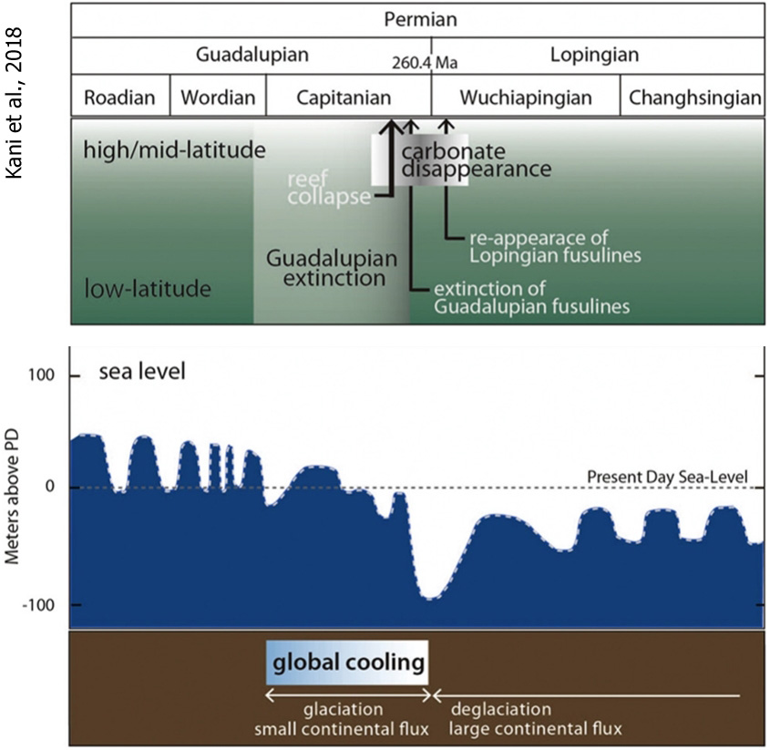
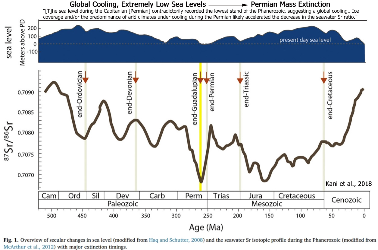


Recent Comments