Collins et al., 2019 Over the past 2300 yrs, SST values range between 14.3°C and 12.2°C (Fig. 4a), and hence most of the record is warmer than today. The earlier half of the record is relatively warm and stable and displays a gradual warming from 13.2°C at 2300 cal yrs BP to 14°C at 1200 cal yrs BP. The largest feature of the record is the cooling transition from 14°C to 12.5°C between 1100 and 600 cal yrs BP. Thisis followed by warming to 13.5°C at 300 cal yrs BP and then cooling to 12.5°C at present day. Multi-centennial variability is more clearly highlighted in the filtered record and is most pronounced over the last 1200 years. The record exhibits relatively warm conditions during the periods 1200 – 950 cal yrs BP and 500 – 200 cal yrs BP and relatively cool conditions during the periods 950 – 500 cal yrs BP and 200 – present. … Southern Ocean cooling is expected to have further enhanced sea ice cover in the Southern Ocean (Park and Latif, 2008; Zhang et al., 2017a). This is in accordance with two records displaying increased sea ice in the western Ross Sea at a similar timing (between 1250 and 650 cal yrs BP) to the cooling (Mezgec et al., 2017). Late Holocene sea-ice increases are also observed to the west of the Ross Sea (Denis et al., 2010), to the west of the West Antarctic Peninsula (Etourneau et al., 2013) and in the Eastern Ross Sea (Mayewski et al., 2013). Associated ice-albedo and ice-insulation feedbacks (Renssen et al., 2005; Varma et al., 2012) may have contributed to the rapidity of the cooling and sea-ice expansion. … Solar variability would be a potential driver of the changes in ENSO and SAM coupling. Increased (decreased) TSI has been shown to promote La-Niñalike (El-Niño-like) conditions by enhancement of the trade winds (Mann et al., 2005). Similarly, the SHW are sensitive to the 11yr solar cycle (Haigh et al., 2005) and solar variability on centennial timescales (Varma et al., 2011) and thus solar variability might be expected to exert an influence on the SAM. Therefore, it is plausible that solar variability may have controlled the phasing of ENSO and the SAM, and this remains an interesting avenue for further climate modeling research.
Lee et al., 2019
Salvatteci et al., 2019 [O]tolith δ18O data from Peruvian catfish (Galeichthys peruvianus) excavated from archeological sites in northern Peru suggest SST ~4 °C warmer than present‐day SST (Andrus et al., 2002).
Liu et al., 2019 The modern vegetation around Tianchi Crater Lake is categorized as temperate mixed conifer-broad-leaved forest … The area experiences a typical cold temperate monsoon climatic regime with long cold winters and short cool summers. The [modern] annual average air temperature is 0–0.5 °C … The PFT-MAT-based reconstructed Pann record for Tianchi Crater Lake has a similar trend of variation to that of the pollen percentage diagram. The ranges of Pann [annual precipitation] and Tann [annual mean temperature] are 268–881 mm and1.7–10.5°C, respectively [for the Holocene]. …[V]ariations in Tann exhibit […] a marked rise from the beginning of the early Holocene and a peak at 9000–8000 cal yr BP.
Klinge and Sauer, 2019 For the Tsambagarav Mountain (central Mongolian Altai), Herren et al. (2013) reconstructed the climatic development over the last 6 ka, based on an ice core. Because the maximal age obtained for the base of the glacier ice was approximately 6 ka, they concluded that warm conditions led to disappearance of most of the glaciers in the Altai Mountains during the early to mid-Holocene. This assumption was supported by Ganyushkin et al. (2018), who found fossil wood above the modern tree line in the Mungun-Taiga Mountain in northwest Mongolia, dating between 10.6 ka and 6.2 ka. They concluded that thetree line was 350 m higher than today at that time, indicating that summer temperatures were 2.0-2.5°C warmer than at present, and MAP was about twice as much as today, which led to a decrease of the glaciated area.
Girardin et al., 2019 Biomass burning fluctuations also significantly co-varied with Greenland temperatures estimated from ice cores, at least for the past 6000 years. Our retrospective analysis of past fire activity allowed us to identify two fire periods centered around 4800 and 1100 BP, coinciding with large-scale warming in northern latitudes and having respectively affected an estimated∼71% and∼57% of the study area. … The p̂CNFD [Canadian National Fire Database] exhibits a drop in 1992–1993, consistent with high-latitude cooling caused by the eruption of Mount Pinatubo (Parker et al 1996), followed by an increase until 2005 that is consistent with Greenland warming (figure S14). For the most recent 11 years on record (2005–2016), Greenland temperature has exhibited a slightly decreasing trend consistent with northern North Atlantic-wide cooling during that period (figure S15) and a slowdown of the Atlantic Ocean overturning circulation (Thornalley et al 2018). The proportion of forest that was affected by extreme biomass burning also declined during this period (figures 1 and S7). … Two periods of high sub-continental biomass burning and p̂CHAR (i.e. 4950–4750 BP and 1250–1050 BP) are found during some of the periods of warmest Holocene temperatures in Greenland (respectively about +2.4 °C and +3.4 °C above the 1951–1980 baseline; figure 4(e); Kobashi et al 2017). Both periods coincide with positive temperature anomalies that have been inferred from chironomid assemblages in eastern boreal North American lakes (∼+2.1 °C and 2.2 °C above baseline (Bajolle et al 2018, figure S11).
Joo et al., 2019 An early Holocene seawater temperature reconstruction for Dicksonfjorden exemplifies an amplified effect of warming (+4–6°C [warmer than present]) at high latitudes relative to global estimates (+1–3°C [warmer than present]; Beierlein et al. 2015). The early Holocene warmth culminated with a stepwise regional cooling, influenced by decreasing insolation, starting at ca. 9–8.8 Kya (Svendsen & Mangerud 1997; Hald et al. 2004; Forwick & Vorren 2009; Rasmussen et al. 2012; Mangerud & Svendsen 2018).
Barhoumi et al., 2019 In North America and Arctic Canada, an early Holocene thermal maximum (from about 8000 to 5000 cal. yr BP) is evidenced with summer temperatures at least 2° warmer than today (Axford et al., 2009; Viau and Gajewski, 2009). In the prepolar and polar Ural regions, the climate was probably moist and warm (summer temperatures c. 4°C warmer than today) between 8000 and 4500 BP (Kultti et al., 2003).
Bogren, 2019 Macrofossil inferred temperatures from indicator plant taxa in northern Fennoscandia indicate that the very beginning of Holocene (between 11000 and 10000 cal. yr BP) had several degrees warmer summer temperatures than present(e.g. Valiranta et al., 2015; Shala et al., 2017), which is also in agreement with what Luoto et al. (2014) found in chironomid-based records in northern Finland.). … Most proxies indicate that a long-term cooling trend started in Fennoscandia during the late Holocene (from c. 5000 cal. yr BP to the present), likely related to the decreased insolation in northern Europe (Borzenkova et al., 2015). … In Abisko in the northern Swedish Scandes the tree-type Betula tree line is suggested to have been at an altitude of 300-400 m higher than present in the early Holocene (Barnekow, 1999; Barnekow and Sandgren, 2001).
Schirrmacher et al., 2019In the Gulf of Cádiz alkenone-based SST values vary between 20.0 to 22.7°C and are warmer compared to recent annual mean temperatures (18.7°C; Locarnini et al., 2013). Higher SSTs during the mid-Holocene might be partly a consequence of higher insolation during this period.
Lacka et al., 2019 Sea ice-free conditions remained during most of the mid-Holocene as a result of the influence of AW [Atlantic Water] (Łacka et al., 2015b). These conditions coincided with the highest Holocene primary productivity observed on the northern continental slope of the Barents Sea (Wollenburg et al., 2004). The northern Barents Sea experiences seasonal sea ice cover that forms during fall/winter (Loeng, 1991). Sea ice breakup occurs during summer, leading to open-water conditions in August and September (Belt et al., 2015). … The SSTs at the study site during the B-A varied between 2°C and 4°C, which is comparable to modern SST values in Storfjordrenna [~3°C]. … Between 9200 cal yr BP and 3400 cal yr BP, SSTs in Storfjordrenna remained highly variable (from 3°C to almost 13°C). At approximately 6400 cal yr BP, the SST in Storfjordrenna reached a peak of almost 13°C[10°C warmer than modern].
Benson et al., 2019 Summer temperatures reconstructed from Burial, Zagoskin, and Trout Lakes using fossil Chironomidae assemblages provide additional evidence of increased summer temperatures (Fig. 7) that were roughly 1–2°C warmer than modern July air temperatures (Kurek et al., 2009b; Irvine et al., 2012). Additional evidence suggesting regionally warm conditions during the early Holocene includes the highest rates of thaw-lake initiation and peat formation ages from 11 to 10 cal ka BP (Jones and Yu, 2010; Walter Anthony et al., 2014).
van der Bilt et al., 2019 Alkenone data show that Svalbard experienced summer temperatures both warmer and colder than today during the Early Holocene. Warmth was greatest around 10 ka BP, when temperatures were up to ~7 °C higher than present in response to high radiative forcing and intensified ocean heat advection. In agreement with a growing body of recent work (e.g. Lecavalier et al., 2017; McFarlin et al., 2018), these findings indicate an earlier and warmer Holocene Optimum in the High Arctic then previously suggested. Supporting these findings, Mangerud and Svendsen (2018) derive a similar amplitude for peak Holocene warmth, based on the presence of Zirfaea crispata, a thermophilous mollusc that is not present in Svalbard waters today. … As seen in Figure 2e, sub-surface temperatures display a prominent peak around 10 ka BP that is unmatched in the remainder of the Holocene. Werner et al. (2015) infer a similar pattern of temperature change in the adjacent eastern Fram Strait. In addition, an IP25 reconstruction from the same site suggests that the seasonal sea ice margin had retreated north of Svalbard at this time. … Placed in a regional context, our findings support a number of recent studies that suggest an earlier, warmer and more distinct Arctic Holocene optimum (Lecavalier et al., 2017; McFarlin et al., 2018). Collectively, this body of work stresses the need for data-model comparisons as simulations neither reproduce this reconstructed pattern nor its magnitude (Figure 2c; Zhang et al., 2018).
Leopold et al., 2019 The warmest phase, referred to as the ‘Holocene thermal optimum’, occurred around 10.7–7.7 kyr. BP, peaking at 10.2–9.2 kyr. BP (Mangerud and Svendsen 2018). Reconstructed summer SSTs were as high as 8 °C during this period and later dropped to around 4 °C where they stabilized and persisted for~ 5 kyr. (Sarnthein et al. 2003). … Even though the summer SSTs today around Svalbard are some 5–8 °C lower than during the thermal peak of the early Holocene, they are well within the temperature range when Mytilus spp. previously occupied the archipelago. The Holocene occurrence of Mytilus spp. was most likely a recurring event during intermittent warm periods (see Mangerud and Svendsen 2018, results and discussion).
Brown et al., 2019 While summers in the interior of BC were 2–4 ºC warmer-than-present (Rosenberg et al., 2004), the coastal regions were probably only 1–2 ºC warmer (Hebda, 1995; Mathewes and Heusser, 1981).
Klippel et al., 2019[A]n analysis of instrumental temperatures forthe period 1955–2013 shows that in northwestern Greece, statistically significant trends in summer temperature are absent (Feidas, 2016). The cooling trend from 1950–1976, previously reported throughout the Mediterranean basin, was followed by an, so far, insignificant warming (Piervitali et al., 1997; del Río et al., 2011). Our reconstruction mirrors this absence of a clear positive trend at decadal scale. … In total, 110 cold and 48 warm extremes appear in the 100SP reconstruction, and 105 cold and 57 warm extremes in the 10SP reconstruction (Figure 5 and Table S1). The year 1240 was the warmest summer, with reconstructed anomalies of +3.13 °C and +2.64 °C in the 100SP and 10SP reconstructions, respectively. The two coldest summers in the 100SP reconstruction are 1217 and 1884 with anomalies of –3.71 °C and –3.61 °C, respectively. The two coldest summers in the 10SP reconstruction occurred in different years, 1035 and 1117, with anomalies of –3.11 °C and -3.14°C, respectively. The third coldest summer in the 100SP and fourth coldest summer in the 10SP reconstructions, is 1959, which is the second coldest year in the instrumental EOBS v.15 record. The coldest decade is 1811–1820 (–0.73°C) and the warmest decade 1481–1490 (+0.88°C; calculated only for 100SP reconstruction). The elimination of decadal trends in the 10SP reconstruction causes events to appear more evenly distributed. However,overthe past 450 years the occurrence of warm temperature extremes is substantially less frequent compared to preceding centuries.
Fletcher et al., 2019 The Pliocene is an intriguing climatic interval that offers important insights into climate feedbacks. Atmospheric CO2 concentrations were, at times, as high as modern ones (Fig. 1), but generally show a decreasing trend throughout the Pliocene (Haywood et al., 2016; Pagani et al., 2010; Royer et al., 2007; Stap et al., 2016), Although CO2 estimates from different methods do not converge, the modeled direct effects of these CO2 discrepancies appear to be small (Feng et al., 2017). Of additional importance for comparability to the modern climate system, continental configurations were similar to present (Dowsett et al., 2016). While global mean annual temperatures (MATs) during the Pliocene were only ∼ 3°C warmer than in the present day, Arctic land surface MATs may have been as much as 15 to 22°C warmer(Ballantyne et al., 2010; Csank et al., 2011a, b; Fletcher et al., 2017). Further, Arctic sea surface temperatures may have been as much as 10 to 15°C warmer than modern ones (Robinson, 2009), and sealevels were approximately 25 m higher than present (Dowsett et al., 2016). As a result, the Arctic terrestrial environment was significantly different from today, with boreal ecosystems at much higher latitudes (Salzmann et al., 2008).
Tamo and Gajewski, 2019Reconstructed July temperatures ranged from 4.5 to 8.0°C and showed a cooling trend of about 1.5°C from 1080–1915 CE and with lowest temperatures (4.5°C) reconstructed between 1800 and 1915 CE. Temperatures rose over the last 100 years to between 5 and 6°C, which is comparable to MCA values (Figure 4). … Other reconstructions with an average temporal resolution of less than 100 years between data points (SL06 and MB01, Peros and Gajewski 2009) and one slightly lower resolution record (JR01, Zabenskie and Gajewski 2007) showed some between-site congruence with SW08 (Figure 6). Two of the sites (SL06 and MB01) recorded warmer temperatures during most of the first millennium, and the longer records showed a centennial-scale cooling trend in the Common Era. All four sites reconstructed a relative cooling between 1800 and 1930 CE when temperatures decreased by 0.5–1.5°C from the mean of the last 1,000 years for each record. Although each site experienced a cold period of similar amplitude, the duration varied between sites. SW08 and SL06 recorded a longer sustained cold period from 1800–1930 CE and 1775–1950 CE, respectively. At SL06, this period was an intensification of colder conditions that began at ~1100 CE, whereas at SW08 there was more variability prior to 1800 CE.
Bobylev and Miles, 2019 The Holocene is the present interglacial period, which has persisted for about 12 kya. The Arctic summer air temperatures during the warmest part of the period were as much as2–3°C above present for much of the region, which was well above the interglacial average temperature for the rest of Earth (Fig. 2.5). Multiple proxy records indicating that early Holocene temperatures were higher than today and that the Arctic contained less ice, are consistent with a high intensity of orbitally-controlled spring and summer insolation that peaked about 11 kya and gradually decreased thereafter. The warming phase after the end of the Younger Dryas was very abrupt and central Greenland temperatures increased by 7°C or more in a few decades (McBean et al. 2004). Arctic summer temperatures were warm enough to melt all glaciers below 5 km elevation, except the Greenland Ice Sheet, which was reduced moderately. The last major ice sheet disappeared from Scandinavia about 8000–7000 BC, while in North America the ice retreated completely at an even later date (Frolov et al. 2009). The continued Holocene climate warming, which culminated in the “Holocene Climatic Optimum” (HCO) of 5–9 kya, was characterized by a significant increase in mean air temperature, which was generally 2–3°C higher in summer compared to present conditions.
Lüning et al.,2019 Until recently, the Antarctic Peninsula and West Antarctica were among the most rapidly warming regions on Earth. Between the 1950s and 1990s temperatures on the Antarctic Peninsula increased by more than 0.3°C/decade (Stenni et al., 2017; Turner et al., 2016; Vaughan et al., 2003), with even higher warming rates reported for Byrd Station in West Antarctica (Bromwich et al., 2013; Bunde et al., 2014; Nicolas and Bromwich, 2014). Since the late 1990s, however, this warming has essentially stalled. Rapid cooling of nearly 0.5°C per decade occurred on the Antarctic Peninsula (Favier et al., 2017; Fernandoy et al., 2018; Turner et al., 2016). This already impacted the cryosphere in parts of the Antarctic Peninsula, including slow-down of glacier recession, surface mass gains of the peripheral glacier and a thinning of the active layer of permafrost in the northern Antarctic Peninsula islands (Engel et al., 2018; Oliva et al., 2017; Seehaus et al., 2018). At the same time, temperatures in West Antarctica over the past two decades appear to have plateaued or slightly cooled (Bromwich et al., 2013; Jones et al., 2016; Steig et al., 2009). However, temperature records in West Antarctica are few, often discontinuous and show opposing trends from location to location (Shuman and Stearns, 2001) which complicates modern trend analysis in this part of Antarctica. In contrast, East Antarctica has not experienced any significant temperature change since the 1950s (e.g. Yang et al., 2018) and some areas appear to have even cooled during the most recent decades (Clem et al., 2018; Favier et al., 2017; Jones et al., 2016; Marshall et al., 2014; Nicolas and Bromwich, 2014; O’Donnell et al., 2011; Ramesh and Soni, 2018). Cooling and an increase in snowfall in East Antarctica seems to have led to a gain in ice sheet mass and thickening of ice rises over the past 15 years (Goel et al., 2017; MartinEspañol et al., 2017; Philippe et al., 2016; Zwally et al., 2015). East Antarctic marine-terminating glaciers show no systematic change over the past 50 years (Lovell et al., 2017). Lastly, also the surface layers of the Southern Ocean south of 45°S has predominantly cooled over that past three decades (Armour et al., 2016; Fan et al., 2014; Kusahara et al., 2017; Latif et al., 2017), whilst the subpolar abyssal waters are warming (Sallée, 2018).
Lin et al., 2019 The mid-Holocene period (MH) has long been an ideal target for the validation of general circulation model (GCM) results against reconstructions gathered in global datasets. Our results indicate that the main discrepancies between model and data for the MH climate are the annual and winter mean temperature. A warmer-than-present climate condition is derived from pollen data for both annual mean temperature ( ∼ 0.7 K on average) and winter mean temperature (∼ 1 K on average), while most of the models provide both colder-than-present annual and winter mean temperature and a relatively warmer summer, showing a linear response driven by the seasonal forcing.
Curran et al., 2019 [R]ecords for the Northgrippian from the East Greenland margin provide no evidence of increased calving of the Greenland Ice-Sheet (Jennings et al., 2002, 2011; Risebrobakken et al., 2011). This is likelydueto the absence of sustained marine-terminating glaciers on the East Greenland margin during the warmer than present Northgrippian(Larsen et al., 2015). … The intervals of warmest BWT [bottom water temperatures] occurred between ca. 4-5 ka and between 2.2 ± 0.1 ka and 2.4 ± 0.2 ka. … Mg/Ca measurements from gravity core GC07 indicate a gradual warming from 11.5°C at 7.5 ± 0.2 ka to reach a maximum of 13.1°C at 4.2 ± 0.2 ka
Axford et al., 2019 Deltasø chironomids indicate peak early Holocene summer temperatures at least 2.5-3°C warmer than modern and at least 3.5-4°C warmer than the pre-industrial last millennium. We infer based upon lake sediment organic and biogenic content that in response to declining temperatures, North Ice Cap reached its present-day size ~1850 AD, having been smaller than present through most of the preceding Holocene.
Jimenez-Moreno et al., 2019 The pollen record is also consistent with higher than modern summer temperatures. Previous studies from the area show that upper treeline would have been between 80 and 300 m higher than today. … Here, we find that low elevation thermophilous species, such as Quercus, Juniperus and Cercocarpus, reached maximum abundances between 8000 and 6700 cal yr BP in subzone EL-2a. This pattern probably points to the occurrence of these species at their highest Holocene elevations at this time and thus adds to evidence for the highest regional temperatures in the middle Holocene, possibly >2°C warmer than today (Andrews et al., 1975; Carrara et al., 1984; Elias, 1996). … A continuous cooling trend over the last few millennia is also recorded at Emerald Lake by a progressive decline in the pollen percentages of Quercus and other thermophilous species such as Juniperus and Cercocarpus. These species probably retreated to lower elevations under colder conditions. Decreasing summer insolation in the late Holocene (Neoglacial) led to cooler summers than earlier in the Holocene (Laskar et al., 2004; Alder and Hostetler, 2015), and most likely caused these vegetation trends.
Reißig et al., 2019 [T]he Tobago Basin core 235 subSSTMg/Ca record is highly variable and ranges from ~13-23°C, which is approximately three times as much as at Beata Ridge.. In Tobago Basin, the subSSTMg/Ca decrease by ~2°C from 30 ka BP (18°C) to the onset of HS1 (16°C). Within HS1, the subSSTMg/Ca increase continuously by 2°C, while at ~15.5 ka it rises abruptly by ~6°C up to maximum temperatures of 23°C. The abrupt subSST rise is delayed too the reconstructed SST rise at the beginning of HS1 by Bahr et al. (2018) (Fig. S7). Subsequently, subSSTMg/Ca scatters around 20°C until the beginning of the Bølling-Allerød (B/A). During the B/A and the YD the subSSTMg/Ca remains higher than ~19°C, abruptly increases up to ~22°C at mid YD, while steadily decreasing afterwards reaching modern values of ~15.5°C in the mid Holocene. Lowest subSSTMg/Ca of ~13°C are observed after ~7 ka BP. On average, the LGM subSSTMg/Ca are warmer by ~2.5°C than during the Holocene. … [T]he subsurface temperature variability is a robust climate signal in the tropical W Atlantic. Both records show an increase of ~5°C in subSSTMg/Ca from the LGM to the early YD and a subSSTMg/Ca decrease by ~7-8°C during the Holocene suggesting that both sediment cores are influenced by the same oceanographic changes. Notably, the mid Holocene subSSTMg/Ca in Tobago and Bonaire Basins remain cooler by ~1.5°C and ~3°C, respectively, than during the LGM. … At Tobago Basin and Bonaire Basin, the deglaciation is characterized by abrupt rises in subSSTMg/Ca by ~5.5°C at the end of HS1 and by ~6°C at the middle of the YD to peak values of up to ~23°C and ~22°C, respectively, accompanied by changes towards saline conditions (mean δ18Osw-ivf of ~2.25‰ and ~2‰, respectively (Fig. 3). These highly variable changes occur within less than 400 years. … In contrast to modern conditions Tobago Basin core 235 was influenced by a warm water mass between 30-10 ka BP, indicated by elevated subSSTMg/Ca (~2.5°C warmer than the modern conditions)
Yasuhara et al., 2019 Our reconstructions reveal a series of multi-centennial-scale abrupt warming events likely caused by upper NADW reduction coinciding with deglacial and Holocene stadial events. Notably, we discovered pervasive Holocene upper NADW variability in the western North Atlantic for at least the past 4000 yr and perhaps throughout the Holocene. Bottom-water temperature at ODP Site 1055 (1798 m) averaged ~5 °C during the last glacial period, which is slightly (by 1 °C) warmer than present-day and late Holocene values of ~4 °C. During the last deglaciation, ODP 1055 BWT shows several warming events supported by multiple data points (apart from noisy, singlepoint excursions). During the Holocene, ODP 1055 BWT shows ±1–1.5 °C multi-centennial-scale variability. Evidence for warmer-than-present lastglacial BWT at 1800 m water depth is consistent with low-resolution depth transect reconstructions (Dwyer et al., 2000).
Tonno et al., 2019 In North Europe, changes in early Holocene climate were rather intense, starting with low temperatures at the beginning of the period, followed by gradual warming, interrupted periodically by short cooling periods (Antonsson and Seppa¨ 2007). During the Holocene Thermal Maximum (HTM), the period from 8.0 to 4.0 cal ka BP, average temperatures in Northern Europe were approximately 2.5–3.5°C higher than today (Antonsson and Seppa¨ 2007; Heikkila¨ and Seppa¨ 2010; Ilvonen et al. 2016).
Pitulko et al., 2019 Our data show that from c. 10 600 BP, Zhokhov Island was situated on the margin of the shrinking Arctic coast (Anisimov et al. 2009); this is supported by the presence of a large quantity of driftwood that washed ashore at the Zhokhov site. The environmental situation was relatively favourable for human occupation: the climate was [5-6°C] warmer than today, and Zhokhov Island was covered by an Arctic tundra comprising sedge grass, shrubs and dwarf birch (Makeyev et al. 2003).
Kusch et al., 2019 High d13C values from Bliss Lake indicate that warmer conditions than today persisted from 7.2 to 6.5 cal. ka BP (Olsen et al. 2011). The records mentioned above imply relative warming during the HTM, but do not provide quantitative constraints on temperature changes. The closest terrestrial, non-ice-core record of absolute temperature change comes from Last Chance Lake in central East Greenland, approximately 1000 km farther south. Axford et al.(2017) D’Andrea et al. (2011) used the alkenone-basedUk’37 palaeothermometer to reconstruct lake water temperatures in two small lakes near Kangerlussuaq, southwest Greenland. Their results show variations of up to 5.5 °C since 5.6 cal. ka BP (D’Andrea et al. 2011). … Interestingly, using a combined MBT’/CBT calibration such as the Peterse et al. (2012) calibration (Table S1) results in a smoothed MAT curve, which shows a relatively constant ~3.7 °C decrease across the Holocene that agrees well with other temperature estimates (e.g. Axford et al. 2017).
Feakins et al., 2019 At lake level [Lake Elsinore, southern California] mean annual temperature (MAT) averages 18°C, with summer average temperatures of 25°C, resulting in high potential evaporation rates and lake water loss of >1.4 m yr−1(Kirby et al., 2013). … [T]he reconstructed temperatures are reasonable with early Holocene values close to modern (18°C). … Temperatures >20°C are reported for six late glacial samples, including a high of 22°C at 29.4 ka and a maximum of 23°C at 26.8 ka which coincides with the pollen-inferred warm and dry period from 27.5–25.5 ka (Heusser et al., 2015) when the lake was shallow (∼3.2–4.5 m deep; Kirby et al., 2018). … The lowest temperature, 10°C, occurs at 23.5 ka and the deglacial warming from 14–12 ka is >10°C, agreeing with the pollen interpretations of ∼11°C warming at the glacial termination (Heusser et al., 2015).
Marret et al., 2019 The studied region is the only coastal region in Russia to have subtropical landscapes as well as humid to semi-arid landscapes (Petrooshina, 2003). Winter temperatures average 3–5°C in winter [today] up to 23–24°C in summer. … A possible maximum of warm conditions may have occurred between 3.0 and 2.5 cal. ka BP, as highlighted by the occurrence of O. israelianum. This species has not been seen in modern sediments from the Black Sea nor the Caspian Sea and mainly occurs in waters where winter SSTs are above 14.3°C and summer SSTs are more than 24.2° C … Establishment of present-day conditions may have happened within the last 1500 years, but the low-resolution sampling at the top of the core prevents us to exactly pinpoint this change. However, our dinocyst assemblage indicates cooler conditions [today] with the decrease of S. mirabilis.
Røthe et al., 2019 Our findings do not provide any confirmation that the glacier Sørfonna melted entirely away during the Holocene Thermal Maximum (HTM). Bjune et al. (2005) suggest summer temperatures were 1.5–2 °C warmer than present during this period. Combined with the evidence from the glaciers Nordfonna and Hardangerjøkulen, it is, however, likely that the glacier Sørfonnawas also significantly smaller than at present during this period. … Since 1650 cal. a BP, we infer that the glacier was larger than the 2002 CE glacier extent until 1910 CE when a GLOF [glacier outburst flood] occurred. Svartenutbreen has been retreating since 1910 CE, which led to the ice damming of the two historical GLOFs [glacier outburst floods] in the 1980s and 2002 CE separated by a glacier advance in the 1990s CE.
Colin et al., 2019The Holocene subpolar North Atlantic climate is characterized by an early to mid-Holocene “thermal maximum” followed byprogressive cooling induced by decreased insolation forcing (related to orbital precession) (e.g. Marchal et al., 2002; Sarnthein et al., 2003). This climatic cooling reflects a major reorganization of atmospheric and ocean circulation in the North Atlantic (e.g. O’Brien et al., 1995; Came and Oppo 2007; Repschlager et al., 2017). … The time interval from 1 to 0.68 ka BP, which is marked by a strong eastward extension of the SPG, has been associated with the warm Medieval Climatic Anomaly and a subsequent intensification of the surface limb of the AMOC (Copard et al., 2012; Wanamaker et al., 2012; Ortega et al., 2015) (Fig. 4). The westward contraction of the weak SPG observed thereafter (between 0.68 and 0.2 ka BP) is coeval with the cold period of the Little Ice Age and may be linked to reduced AMOC intensity.
Steinman et al., 2019 The early Holocene d18O [hydroclimate] maximum in the Castor Lake record at 9630 (9110-10,100) yr BP is likely in part a result of higher summer insolation, which produced higher temperatures and greater evaporation during the warm season. Additionally, atmospheric circulation in the early Holocene was substantially different from the modern configuration (Bartlein et al., 2014), and precipitation amounts were likely lower, due to the presence of the residual Laurentide and Cordilleran Ice Sheets (Dyke, 2004), which affected air mass trajectories and the seasonal distribution and amount of precipitation on a hemispheric scale. … A chironomid based climate reconstruction from Windy Lake, south-central British Columbia, supports the assertion that greater summer insolation produced warmer summer temperatures at this time (Chase et al., 2008).
Wetterich et al., 2019 To reconstruct Holocene temperature changes, Lasher et al. (2017) employed δ18O of chironomid head capsules from Secret Lake in the Thule District as a proxy for the δ18O of precipitation, which is further related to surface air temperature. This proxy approach yields maximum estimates of Holocene temperature changes but is, as the study states, biased in summer and early autumn. The inferred summer season temperatures that were up to 4 °C warmer than today decreased from about 7.7 until about 2.3 ka cal BP before reaching colder than today temperatures, including the coldest period after about 1.2 ka cal BP (Lasher et al., 2017). The reconstructed period of decreasing summer temperatures covers the onset of permafrost aggradation at both sites, on Appat and at Annikitisoq, and likely relates to the dynamics of the NOW as reflected in sea surface temperature (SST), sea surface salinity (SSS), and sea ice cover (SIC) proxy data from marine sediments such as dinocyst records (Levac et al., 2001). After the breakup of perennial sea ice cover in the northern Baffin Bay around 10.5 ka cal BP, Holocene minima in SIC with up to 4–5 ice-free months per year occurred between about 7.4 and 4 ka cal BP accompanied by maxima in August SST and SSS (Levac et al., 2001).
Tanhuanpää et al., 2019 The postglacial expansion of hazelnut happened in the Holocene epoch, mainly during the Sub-Boreal climatic stage about 6000–4000 years ago, when climate was 2–4 °C warmer than present (Eriksson et al. 1991).
Manzanilla-Quiñones et al., 2019 (North America) Given the recent diversification of the genus Abies in the world (Xiang et al., 2015), it is very likely that climatic conditions of 6 000 to 12 000 years ago were warmer (+2 °C) in North America’s temperate and cold areas (Caballero et al., 2010; Svensson et al., 2008).
Lozhkin et al., 2019 Mixed Larix-Betula forest was established at the Tanon site by ∼6600 14C BP (∼7500 cal BP). This forest included Betula platyphylla, a species common in moderate zones of the Russian Far East (e.g., B. platyphylla-Larix forests of central Kamchatka). The importance of Betula in the Middle Holocene assemblage is unusual, as tree Betula is not a common element in the modern coastal forest. The abundance of B. platyphylla macrofossils particularly suggests warmer than present summers and an extended growing period. This inference is supported by a regional climate model that indicates a narrow coastal region where the growing season was longer and summer temperatures were 2-4 °C warmer than today. Variations in Betula pollen percentages at other sites in northern Priokhot’ye are suggestive that this Middle Holocene forest was widespread along the coast.
Novenko et al., 2019 [D]uring the Holocene Thermal Maximum when the mean annual temperatures were 2°С higher than those of the present day. Roughly 5.7–5.5 ka BP, the Holocene Thermal Maximum was followed by gradual climatic cooling that included several warming and cooling phases with temperature fluctuations ranging between 2 and 3°С. …The CFSNBR [Central Forest State Natural Biosphere Reserve] is situated roughly 360 km northwest of Moscow (the Tver region, 56º35’ N, 32º55’ E) in an ecological zone transitioning from taiga to broadleaf forests. The vegetation of the CFSNBR is primary southern taiga forests, and it has been undisturbed by any human activities for at least 86 years. The climate of the study area is temperate and moderately continental with a mean annual temperature of 4.1°C and annual precipitation of roughly 700 mm.
Rey et al., 2019 Our results imply that mixed Fagus sylvatica forests with Abies alba and Quercus may re‐expand rapidly in these areas, if climate conditions will remain within the range of the mid‐Holocene climatic variability (with summers c. +1–2°C warmer than today). … [T]he rise and fall of early farming societies was likely dependent on climate. Favourable climatic conditions (i.e. warm and dry summers) probably led to an increase in agricultural yields, the expansion of farming activities and resulting forest openings, whereas unfavourable climatic conditions (i.e. cold and wet summers) likely caused crop failures, abandonment of agricultural areas and forest succession. A better understanding of the environmental and societal factors controlling coeveal land-use dynamics as shown in this study would require new climate proxy data (e.g. temperature reconstruction from well dated and complete Holocene tree ring series). On the basis of our results and considering the ongoing spread of temperate forests in lowland Central Europe, we conclude that the existing beech forest ecosystems are resilient to anthropogenic disturbances under a changing climate.
Eda et al., 2019 Recent taxonomic composition and faunal distribution patterns support recognition of three biogeographic regions in Asia, Palaearctic (north), Indomalayan (south), and a transition zone between the two (Hoffmann 2001). In the division, the Yangtze River delta is located at the boundary of the Indomalayan region and transition zone. Pollen records suggest that, middle Holocene temperatures were ca. 2–4 °C warmer than today in the middle Yangtze River delta (Yi et al. 2003). Peters et al. (2016) indicated that the middle Yangtze River basin would delimit the northern most boundary for required habitat of (sub-) tropical red junglefowl during the Holocene thermal optimum. Furthermore, Xiang et al. (2014) reported that the wild distribution area of red junglefowl extended to northern China in the early Holocene, and domestic chicken farming began in the region.
Yuan et al., 2019 During the early Holocene (10.0–6.0 ka), the modern-type circulation system was not established, which resulted in strong water column stratification; and the higher sea surface temperature (SST) might be associated with the Holocene Thermal Maximum (HTM). The interval of 6.0 to 1.0/2.0 ka displayed a weaker stratification caused by the intrusion of the Yellow Sea Warm Current (YSWC) and the initiation of the circulation system. A decreasing SST trend was related to the formation of the cold eddy generated by the circulation system in the ECS. During 1.0/2.0 to 0 ka, temperatures were characterized by much weaker stratification and an abrupt decrease of SST caused by the enhanced circulation system and stronger cold eddy, respectively.
Lasher and Axford, 2019 More positive δ18O values are found between 900 and 1400 CE, indicating a period of warmth in South Greenland superimposed on late Holocene insolation-forced Neoglacial cooling, and thus not supporting a positive NAO anomaly during the MCA. Highly variable δ18O values record an unstable climate at the end of the MCA, preceding Norse abandonment of Greenland. The spatial pattern of paleoclimate in this region supports proposals that North Atlantic subpolar ocean currents modulated South Greenland’s climate over the past 3000 yr, particularly during the MCA. Terrestrial climate in the Labrador Sea and Baffin Bay regions may be spatially heterogeneous on centennial time scales due in part to the influence of the subpolar gyre.
Gebbie and Huybers, 2019 The ongoing deep Pacific is cooling, which revises Earth’s overall heat budget since 1750 downward by 35%. … In the deep Pacific, we find basin-wide cooling ranging from 0.02° to 0.08°C at depths between 1600 and 2800 m that is also statistically significant. The basic pattern of Atlantic warming and deep-Pacific cooling diagnosed from the observations is consistent with our model results, although the observations indicate stronger cooling trends in the Pacific. …. At depths below 2000 m, the Atlantic warms at an average rate of 0.1°C over the past century, whereas the deep Pacific cools by 0.02°C over the past century. … Finally, we note that OPT-0015 indicates that ocean heat content was larger during the Medieval Warm Period than at present, not because surface temperature was greater, but because the deep ocean had a longer time to adjust to surface anomalies. Over multicentennial time scales, changes in upper and deep ocean heat content have similar ranges, underscoring how the deep ocean ultimately plays a leading role in the planetary heat budget.
Helmens, 2019 Quantitative climate reconstructions based on pollen from terrestrial plant taxa show mean July temperature values reaching 3 °C warmer than the present-day value of +13 °C at Sokli.
Ning et al., 2019 Here we investigate the sources of branched glycerol dialkyl glycerol tetraethers (brGDGTs) in Lake Ximenglongtan from southwestern China and present a brGDGTs-based Holocene (~9.4 cal kyr BP) temperature reconstruction. Holocene temperature evolution is characterized by an early cool phase (with a mean annual air temperature (MAAT) of 12.5 °C) prior to 7.6 cal kyr BP, followed by a rapid warming towards the local thermal maximum (MAAT = 13.8 °C) from 7.6 to 5.5 cal kyr BP and a subsequent long-term cooling that ended at 1.5 cal kyr BP. Temperature changes after 1.5 cal kyr BP show high variability and low correspondence to global climate events such as the Medieval Warm Period. Overall Holocene temperature variation has been primarily controlled by boreal summer insolation changes.
Caballero et al., 2019 Diatom-based transfer functions for salinity, precipitation and temperature were developed using a training set that included data from 40 sites along central Mexico. … Maximum last glacial cooling of ∼5°C is reconstructed, a relatively wet deglacial and a warmer (+3.5°C) early Holocene. … The early Holocene marked a change towards high lake salinities andthe highest positive temperature anomalies (+3.5°C) during a peak in summer insolation.
Emslie and Meltzer, 2019 Ultimately, however, the most significant changes in climate and biota in the UGB [Upper Gunnison Basin, Colorado] occurred in the Early to Middle Holocene, when incoming solar radiation peaked, summer temperature increased, and effective precipitation decreased. As a result, biotic communities changed: the upper tree line shifted upslope to perhaps 270 m higher than today (Fall,1997b).
Aguirre et al., 2019 A SST rise of ca. 1-2°C during the Hypsithermal (ca. 7.5-4.5 ka B.P.) in comparison with the modern average oceanic temperaturesis independently supported by the palaeobiogeographical pattern of stenothermal gastropods and bivalves northwards displaced at present (“anomalous taxa”; Aguirre, 1993, Aguirre et al., 2011, 2017) together with the absence of the cold gastropod T. atra (Aguirre et al., 2013) and is sufficient to have displaced winds, shallow water masses and the Brazil Malvinas Confluence southwards along Patagonia. … The mid-Holocene and Last Interglacial were warmer than today due to a southward shifted BMC, stronger and poleward shifted southern westerlies winds, enhanced ACC and subantarctic shelf water, and intensified ocean fronts/upwelling levels.
Lasher and Axford, 2019 More positive δ18O values are found between 900 and 1400 CE, indicating a period of warmth in South Greenland superimposed on late Holocene insolation-forced Neoglacial cooling, and thus not supporting a positive NAO anomaly during the MCA. Highly variable δ18O values record an unstable climate at the end of the MCA, preceding Norse abandonment of Greenland. The spatial pattern of paleoclimate in this region supports proposals that North Atlantic subpolar ocean currents modulated South Greenland’s climate over the past 3000 yr, particularly during the MCA. Terrestrial climate in the Labrador Sea and Baffin Bay regions may be spatially heterogeneous on centennial time scales due in part to the influence of the subpolar gyre.
Svare, 2019 Seppä et al. (2008) set the summer temperature maximum in the northern European tree-line region to ca. 7500-6500 cal. yrs BP (ca. 1.5°C higher than present), similar to the Dovre area (Paus et al., 2011). Further, Bjune et al., (2005) found the HTM to last from ca. 8000 to 4000 cal. yrs BP in Western Norway, with temperatures reaching 12-13°C. … The early establishment of pine-forests in the area surrounding both study sites from ca. 9600 cal. yrs BP give evidence of local mean July temperatures of at least 11°C ca. 9600-8200 cal. yrs BP, 0.8-1.1°C warmer than present. From ca. 8200 cal. yrs BP until present day the July mean temperature has presumably been around 8-10°C.
Kuzmina et al., 2019Even during coldest time of the Pleistocene, the Last Glacial Maximum (LGM), summer temperatures were higher here than they are today (Alfimov, Berman, 2001, Alfimov et al., 2003). … The Pleistocene megafauna of the North Slope was dominated by mostly horses … There are depressions in the main Pleistocene unit filled by early Holocene sediments containing well-preserved leaves, logs and stumps of Populus balsamifera. Since the modern limit of this tree species is south of the North Slope, the presence of fossil poplar indicates warmer than present climate during the early Holocene. … The second warming (around 9–8 ka), which corresponds with Boreal Period of the BlyttSernander scheme, was probably the warmest interval of the Holocene in Beringia (Kaufman et al., 2004). Trees spread north to coastal areas in Siberia (Kaplina, Lozhkin, 1982; Kuzmina, Sher, 2006), spruce forest reached the central Brooks Range (Anderson, Brubaker, 1994), and beaver occupied formerly treeless landscapes in Alaska (Robinson et al., 2007). Climate on the North Slope was about 2 to 3°C warmer than today; and moisture was lower (Nelson, Carter, 1987).
Rull et al., 2019 (Pantepui, NE South America) Myrica forests dominated during the HTM [Holocene Thermal Maximum] and reached their maximum importance at the end of this phase. A sudden replacement of these forests by tepui meadows dominated by Stegolepis took place after the HTM, just at the beginning of the regional cooling and drying trend initiated at B6 cal kyr BP. Myrica forests never returned to the site. The only species of this genus living today in the Guiana region, Myrica rotundata, is endemic to Pantepui and occurs on the slope forests of the Apakara´-tepui, with an upper distribution limit near the coring site (Miller, 2001). It has been suggested that during the HTM, warmer and wetter climates would have favored upslope migration of Myrica forests to higher elevations, which could explain their dominance in the Apakara´ summit. The subsequent post-HTM cooling would have returned Myrica to lower elevations favoring the local expansion of meadows. HTM climatic conditions never recovered during the rest of the Holocene, and Myrica remained at lower elevations until today (Rull and Montoya, 2017)
Hvidberg et al., 2019 Here we present results from a study of the evolution of the Greenland ice sheet through the Holocene (Nielsen et al. 2018). We use a suite of different ice-core-derived climate histories for the Holocene to investigate the evolution of the Greenland ice sheet through the deglaciation, the Holocene thermal maximum and up to present day. The Holocene thermal maximum was a period 8–5 kyr ago when annual mean surface temperatures in Greenland were 2–3°C warmer than present-day values. We use climate histories based on new interpretations of the isotope records (Gkinis et al. 2014), which results in a more pronounced thermal maximum compared to previously used climate records. Furthermore, our records inform of snow accumulation rates in the early Holocene. Our studies show that the Greenland ice sheet retreated to a minimum volume of up to ∼1.2 m sea-level equivalent smaller than present in the early or mid-Holocene, and that the ice sheet has continued to recover from this minimum up to present day.
Warming Since Mid/Late 20th Century?
Kutta and Hubbart, 2019 Between 1900 and 2016, climatic trends were characterized by significant reductions in the maximum temperatures (−0.78°C/century; p = 0.001), significant increases in minimum temperatures (0.44 °C/century; p = 0.017) [overall -0.34°C per century], and increased annual precipitation (25.4 mm/century) indicative of a wetter and more temperate WV climate. Despite increasing trends of growing degree days during the first (p ≤ 0.015) and second half of the period of record, the long-term trend indicated a decrease in GDD [warm growing degree days] of approximately 100 °C/days.
Byambaa et al., 2019 [T]he recent cool-moist period from 1985 to 2000 has been related to the Arctic Oscillation (this study, Robock, 1984, He et al., 2017). The recent cooling could have been caused by volcanic aerosols of the El Chichón eruption (VEI5, 1982) in Southern Mexico, which impacted atmospheric wind patterns, including a positive phase of the Arctic Oscillation (Robock, 1984). No large volcanic-induced cooling was observed at this time due to the simultaneous warming ocean temperature caused by El-Niño (Robock, 2002). Also, the positive AO competing with ElNiño could reinforce the anomalous westerlies in the midlatitudes (He et al., 2017). During this recent cool-moist period, ice mass accumulation of the glaciers in the Russian Altai Mountains was observed and Narozhniy and Zemtsov (2011) connected this phenomenon to annual precipitation increased by 8% – 10% especially in winter and spring (April-May) as a result of a strengthening of the zonal circulation over the Altai Mountains.
Eck et al., 2019 A majority (12/14) of the regions within the SAM [southern Appalachian Mountains] have experienced a long‐term decline in mean winter temperatures since 1910.
Gan et al., 2019 Daily Minimum temperature (Tmin) is an important variable in both global and regional climate changes, and its variability can greatly affect the ecological system. In the early 21st century, warming slowdown is seen over the North Hemisphere and North America is one of the major cooling centers. … In this study, we found that Tmin experienced an obvious decline in North America during warming slowdown period. Such Tmin decline is closely related to the Atlantic Multidecadal Oscillation (AMO), the correlation between the decadal components of Tmin and AMO reached 0.71 during 1950-2014.
Araźny et al., 2019 Air temperature in 1899–1914 during three expeditions was 1.8–4.6 °C lower than the modern period in winter (Oct–Apr). However, during the 1930/31 expedition it was 4.6 °C warmer than the years 1981–2010. Our results relate to what has been called the ‘1930s warming’, referred to by various authors in the literature as the ETCW or the ETCAW. … In individual months, the highest negative anomalies were identified in Calm Bay (hereafter CB) in January 1914 (− 7.4 °C) and in February 1900 (− 6.8 °C). In contrast, duringthe 1930/31 expedition, it was 4.6 °C warmer than the present day in CB [Calm Bay]. Such a high thermal anomaly was influenced by a warm autumn and winter,especially February 1931, when the average monthly temperature was 10.7 °C higher than in the modern period.
Zhang et al., 2019 In core 31003, the SST record shows a distinctly anti-phase relationship with that of core 38002 over the last millennium. For instance, from the MWP to LIA, SST values increased from ∼17.0 ± 0.3°C to ∼19.1 ± 0.6°C in the northern core 38002 but decreased from ∼24.3 ± 0.4°C to ∼23.5 ± 0.3°C in the southern coastal core 31003. Since ∼1850 AD, the SST record in core 31003 elevated within the range of 24.3 ± 0.4°C, similar to values during the MWP, but decreased gradually to ∼18.0°C in core 38002, in line with the SST trends at two additional locations from the YSWC [Yellow Sea Warm Current] pathway as reported by He et al. (2014).
Huang et al., 2019The temperature effect of the Zhada δ18OTR series is further verified by consistency with nearby ice-core δ18O variability.
Watanabe et al., 2019 [P]revious studies have observed that global surface air-temperatures remained relatively constant between the late-1990s and 2015, although climate models predicted continued anthropogenic warming. This so-called global-warming hiatus has received considerable attention [Kosaka et al., 2013]. Satellite-based SST data suggest that the main cause of the global-warming hiatus is the Interdecadal Pacific Oscillation (IPO), which is the dominant mode of atmosphere-ocean interactions in the subtropical Pacific. The IPO reversed from a positive to a negative phase in the late 1990s, i.e. the timing of the IPO phase change coincides with the onset of the global-warming hiatus. The negative IPO led to anomalous cooling in the eastern Pacific and this is thought to be a major cause of the global-warming hiatus. … The 26-year SSTanom record shows a significant regime shift in October 1996 (peak: 0.202; P < 0.01: Fig. 2b). The mean (range) of SSTanom is 0.73 ± 2.59 °C (10.96 °C) before 1996 and −0.46 ± 2.71 °C (11.72 °C) after 1996 (Fig. 2b). SST anom (δ18OSW-anom) shows a gradual cooling (decrease) over the past-26 years (−0.03 ± 0.01 °C/year and −0.02 ± 0.00‰VSMOW/year, respectively).
Booker et al., 2019 Warm Period 1 (~1924–2006 CE) was characterized by Tcal from 23 to 34°C (average 28.3 ± 0.96 °C), which is similar to the current seawater temperature for Grand Cayman and significantly warmer than CP 2. During this period there were two warm intervals (WI 2: ~1924–1932, WI 3: ~1972–1993) and two cool intervals (CI 3: ~1960–1972, CI 4: ~1993–2006). The warm intervals are characterized by an increase in Tcal of ~5–7 °C. The cool intervals are characterized by a decrease of ~4–5 °C. … • Mild Period 1 (~2006–2014 CE) was characterized by Tcal of 25 to 33 °C (average 27.5 ± 0.96 °C) which is similar to the current average seawater temperature for Grand Cayman (t-test: p b 0.01; Fig. 14).
Fröb et al., 2019 The container vessel M/V Nuka Arctica, owned by Royal Arctic Line, operates between Ilulissaat, Greenland and Aalborg, Denmark. … The SST measurements on Nuka Arctica show a substantial cooling during winters between 2004 and 2017(Figures 2c and S6). From the IRM-W through the ICE-W box, the SST trend varies between -0.084±0.020 and -0.096±0.018 ◦C yr−1. Towards the east, thecooling is less pronounced, and in the FB box, the SST trend is only -0.045±0.016 ◦C yr−1. Averaged over all boxes, SST decreased by 0.78±0.19◦C per decade.
Huang et al., 2019 Climatic change is exhibiting significant effects on the ecosystem of the Tibetan Plateau (TP), a climate-sensitive area. In particular, winter frost, freezing events and snow avalanche frequently causing severe effects on ecosystem and social economy, however, few long-term winter temperature records or reconstructions hinder a better understanding on variations in winter temperature in the vast area of the TP. In this paper, we present a minimum winter (November–February) temperature reconstruction for the past 668 years based on a tree-ring network (12 new tree-ring chronologies) on the southeastern TP. The reconstruction exhibits decadal to inter-decadal temperature variability, with cold periods occurring in 1423–1508, 1592–1651, 1729–1768, 1798–1847, 1892–1927, and 1958–1981, and warm periods in 1340–1422, 1509–1570, 1652–1728, 1769–1797, 1848–1891, 1928–1957, and 1982–2007. … It also shows the possible effects of volcanic eruption and reducing solar activity on the winter temperature variability for the past six centuries on the southeastern TP.
Vermassen et al., 2019 A link between the physical oceanography of West Greenland and Atlantic SSTs has indeed been suggested previously: a positive phase of the AMO [Atlantic Multidecadal Oscillation] is related to an increase of warm Atlantic waters flowing towards and along the SE and W Greenland shelf (Drinkwater et al., 2014; Lloyd et al., 2011). … Despite differences in the timing and magnitude of the retreat of the different glaciers, they broadly share the same retreat history.High retreat rates occurred between the mid ‘30s and mid ‘40s (400-800m/yr), moderate retreat rates between 1965-1985 (~200 m/yr, except for Upernavik) andhigh retreat rates again after 2000 (>200 m/yr). … Since the meridional overturning circulation strength and associated heat transport is currently declining, (Frajka-Williams et al., 2017), this may lead to cooling bottom waters during the next decade in Upernavik Fjord and most likely also other fjords in West-Greenland.
Deng et al., 2019 Recent SST records based on longchain alkenones imply that the MCA [Medieval Climate Anomaly] was slightly warmer than the CWP [Current Warm Period] in the northern SCS [South China Sea] (Kong et al., 2017). … [I]t still should be noted that the SST record reconstructed from a Tridacna gigas Sr/Ca profile by Yan et al. (2015a) suggested that the annual average SST was approximately 0.89°C higher during the MCA[Medieval Climate Anomaly] than that of the CWP[Current Warm Period].
Zhang et al., 2019 Natural variability of Southern Ocean convection as a driver of observed climate trends …Observed Southern Ocean surface cooling and sea-ice expansion over the past several decades are inconsistent with many historical simulations from climate models. Here we show that natural multidecadal variability involving Southern Ocean convection may have contributed strongly to the observed temperature and sea-ice trends.
Etourneau et al., 2019 Based on water stable isotopes calibrated to recent air temperatures [Abram et al., 2013, Mulvaney et al., 2012], the reconstructed mean annual SAT documents a 1.5 °C cooling over the Holocene occurring in two steps between 10,000 and 6000 years before present (BP), and 3500 and 500 years BP. The Holocene cooling was interrupted by a slightly warmer period. The first main cooling episode corresponds to a phase of major EAP [East Antarctic Peninsula] ice shelf retreat reported in the literature [Domack et al., 2005, Cofaigh et al., 2014, Johnson et al., 2011, Davies et al., 2012]. … The Larsen A ice shelf was probably destabilized at least as early as ~6300 years BP [Brachfeld et al., 2003], while evidence show that the Larsen B ice shelf experienced a continuous and significant shrinkage throughout the Holocene [Domack et al., 2005]. Hence, the EAP ice shelves underwent a major retreat mostly between ~8000 and 6000 years BP. … [T]he ice core-derived SAT were overall warmer throughout the Holocene than during the last two millennia and could have hence favored the EAP [East Antarctic Peninsula] ice shelf surface melting during the entire period. … The long-term SOT [subsurface ocean temperatures] increasing trend at the JPC-38 core site was punctuated by up to 1.5 °C warm events at the centennial scale.
Li and Luo, 2019The surface air temperature over the Eurasian continent has exhibited a significant cooling trend in recent decades (1990–2013), which has occurred simultaneously with Arctic warming and Arctic sea ice loss. While many studies demonstrated that midlatitude cold extremes are linked to Arctic warming and Arctic sea ice loss, some studies suggest that they are unrelated. The causal relationship between midlatitude cold extremes and Arctic change is uncertain, and it is thus an unsolved and difficult issue. … Arcticwarming or sea ice decline is not necessary for the occurrence of midlatitude cold extremes.
Lack Of Anthropogenic/CO2 Signal In Sea Level Rise
Parker, 2019 Japan has strong quasi-20 and quasi-60 years low frequencies sea level fluctuations. These periodicities translate in specific length requirements of tide gauge records. 1894/1906 to present, there is no sea level acceleration in the 5 long-term stations. Those not affected by crustal movement (4 of 5) do not even show a rising trend. … In Japan tide gauges are abundant, recording the sea levels since the end of the 19th century. Here I analyze the long-term tide gauges of Japan: the tide gauges of Oshoro, Wajima, Hosojima and Tonoura, that are affected to a lesser extent by crustal movement, and of Aburatsubo, which is more affected by crustal movement. Hosojima has an acceleration 1894 to 2018 of +0.0016 mm/yr2. Wajima has an acceleration 1894 to 2018 of +0.0046 mm/yr2. Oshoro has an acceleration 1906 to 2018 of −0.0058 mm/yr2. Tonoura has an acceleration 1894 to 1984 of −0.0446 mm/yr2. Aburatsubo, has an acceleration 1894 to 2018 of −0.0066 mm/yr2. There is no sign of any sea level acceleration around Japan since the start of the 20th century. The different tide gauges show low frequency (>10 years) oscillations of periodicity quasi-20 and quasi-60 years. The latter periodicity is the strongest in four cases out of five. As the sea levels have been oscillating, but not accelerating, in the long-term-trend tide gauges of Japan since the start of the 20th century, the same as all the other long-term-trend tide gauges of the world, it is increasingly unacceptable to base coastal management on alarmist predictions that are not supported by measurements. … The Japan Meteorological Agency (2018) has shown that the relative rise in sea level on the coast of Japan has stabilized since the beginning of the 20th century and has not accelerated. The analysis presented here has further strengthened this result. … The relative sea level rise measured by a tide gauge has a sea and a land component. The relative sea level may rise, or fall, not only because the volume of the water is increasing, or reducing. It may also rise, or fall, because the tide gauge instrument is sinking, or uplifting. The sea component has important multi-decadal periodicities of quasi 60 years. Hence, not less than 60 years of data are needed to infer a rate of rise, and many more years, not less than 100 years, are needed to infer an acceleration.
Duvat, 2019 This review first confirms that over the past decades to century, atoll islands exhibited no widespread sign of physical destabilization by sea level rise. The global sample considered in this paper, which includes 30 atolls and 709 islands, reveals that atolls did not lose land area, and that 73.1% of islands were stable in land area, including most settled islands, while 15.5% of islands increased and 11.4% decreased in size. Atoll and island areal stability can therefore be considered as a global trend. … Importantly, islands located in ocean regions affected by rapid sea-level rise showed neither contraction nor marked shoreline retreat, which indicates that they may not be affected yet by the presumably negative, that is, erosive, impact of sea-level rise. … It is noteworthy that no island larger than 10 ha decreased in size, making this value a relevant threshold to define atoll island areal stability. … [A]mong the 27 islands having a land area lying between 100 and 200 ha (9 in French Polynesia, 6 in the Marshall Islands, 6 in Kiribati, 5 in Tuvalu and 1 in the Federated States of Micronesia), only 3 increased in area, while 24 were stable. … The great majority of Pacific islands showed positional stability, as illustrated by the Tuamotu atolls, where 85–100% of islands were stable, depending on atolls (Duvat & Pillet, 2017; Duvat, Salvat, et al., 2017). … Importantly, the reanalysis of available data on atoll island planform change indicates that over the past decades to century, no island larger than 10 ha and only 4 out of the 334 islands larger than 5 ha (i.e., 1.2%) underwent a reduction in size.
Zhai et al., 2019 To estimate the resilience influences on 15 islands in Florida Bay (Florida, U.S.), our study used indicators (areas of the 15 islands and their mangrove forests) by analyzing 61-yr high-resolution historical aerial photographs and a 27-yr time-series of Landsat images. … Comparative spatial analysis of the historical aerial images showed that the island area significantly increased from 1953 to 2014. For example, Joe Kemp Key had the largest area increase from 0.34 km2 to 0.37 km2. Moreover, the similar increased patterns of island area were found for annual total areas of the 15 islands from 1984 to 2011by analysis of Landsat images. The total areas showed a significant increasing pattern with time. Therefore, results from the analysis of both aerial and satellite images revealed increases in island area, which indicate the island resilience to inundation caused by SLR. However, three islands […] decreased in area. … The long-term island area increases estimated by our analysis supported the resilience of Florida Bay islands to SLR inundation. Moreover, both the positive relationship between the increases of island area and mangrove expansion, and previous field studies in the Florida Bay and nearby Caribbean mangroves suggested the contribution of the mangrove expansion were at the expense of non-mangrove habitats.
Mörner, 2019[T]he Late Holocene and present sea level changes are dominated by the horizontal redistribution of oceanic water masses primarily driven by planetary beat. The future changes in sea level are estimated at a maximum of + 20 cm by the year 2100.
Derrick, 2019 Sea levels in and around 1886 to 2018 … There has been no significant sea level rise in the harbour for the past 120 years, and what little there has been is about the height of a matchbox over a century. Along the northern beaches of Sydney, at Collaroy there has been no suggestion of any sea level rise there for the past 140 years. Casual observations from Bondi Beach 1875 to the present also suggest the same benign situation.
Parker and Ollier, 2019Over the past decades, detailed surveys of the Pacific Ocean atoll islands show no sign of drowning because of accelerated sea-level rise. Data reveal that no atoll lost land area, 88.6% of islands were either stable or increased in area, and only 11.4% of islands contracted. The Pacific Atolls are not being inundated because the sea level is rising much less than was thought. The average relative rate of rise and acceleration of the 29 long-term-trend (LTT) tide gauges of Japan, Oceania and West Coast of North America, are both negative, −0.02139 mm yr−1 and −0.00007 mm yr−2 respectively.Since the start of the 1900s, the sea levels of the Pacific Ocean have been remarkably stable.
Hamlington et al., 2019 Of particular note are mass losses in eastern Brazil, southeastern United States, northern Europe, western Australia, and the southeastern Africa, and massgains [ice] in central India, southeast Asia, eastern Australia, the Nile headwaters, western tropical Africa, northern Great Plains, and northern and southern portions of Brazil. These results are in general agreement with the GRACE trends attributed to natural variability in Rodell et al. [2018], although it should be noted that there are a number of other areas with trends here that are not picked out as attributable to natural variability in the referenced study. … In general, the warm phase of ENSO leads to an increase in global sea level on the order of several millimeters on intraseasonal timescales and the cold phase leads to a decrease of similar magnitude on the same timescales. On the regional level, ENSO variability can lead to rises and falls on the order of tens of centimeters with the largest events causing shifts in coastal sea level that approach half a meter(e.g. in the tropical Pacific). … In summary, there are a number of notable results from our combined CSEOF analysis: 1.The trends in total sea level, steric sea level, and land mass over the period from 2004-2016 are heavily influenced by natural variability. Given the record length, this is unsurprising, but the analysis conducted here does appear to separate much of the natural variability from the background trend that may be expected to persist into the future.
Boretti et al., 2019 There are 20 long-term-trend (LTT) tide gauges along the (Pacific) West Coast of North America. The average relative rate of rise is −0.38 mm/year, and the average acceleration is +0.0012 mm/year². There are 33 LTT tide gauges of the (Atlantic) East Coast of North America. The average relative sea level rise is 2.22 mm/year, and the average acceleration is +0.0027 mm/year². … Sea level acceleration is small, but larger along the East coast, because of the recent subsidence and the recent upward phase of the multi-decadal oscillations that are not phased with those of the West Coast.
Dean et al., 2019Results show RSL in Israel rose from ~0.8 ± 0.5 m at ~2750 a BP (Iron Age) to 0.0 ± 0.1 m by ~1850 a BP (Roman period) at 0.8 mm/a, and continued rising to 0.1 ± 0.1 m until ~1600 a BP (Byzantine Period). RSL then fell to ~0.3 ± 0.1 m by 0.5 mm/a until ~650 a BP (Late Arab period), before returning to present levels at a rate of 0.4 mm/a. The reassessed Israeli record supports centennial-scale RSL fluctuations during the last 3000 a BP, although the magnitude of the RSL fall during the last 2000 a BP is 50% less. The new Israel RSL record demonstrates correspondence with regional climate proxies.
Mörner, 2019 The sea level changes documented in the five equatorial sites investigated: A 20 cm drop in sea level in the mid 20th century (i.e. at the cooling phase after the 1930-1950 warm period in the Northern Hemisphere). Quite stable sea level conditions in the last 50-70 years (i.e. during the period when sea level was rising at a mean rate of 1.1±0.2 mm/yr in the northern Hemisphere).
Armstrong and Lazarus, 2019 [T]rends in recent rates of shoreline change along the U.S. Atlantic Coast reflect an especially puzzling increase in accretion, not erosion. Using U.S. Geological Survey shoreline records from 1830–2007 spanning more than 2,500 km of the U.S. Atlantic Coast, we calculate a mean rate of shoreline change, prior to 1960, of −55 cm/year (a negative rate denotes erosion). After 1960, the mean rate reverses to approximately +5 cm/year, indicating widespread apparent accretion despite steady (and, in some places, accelerated) sea‐level rise over the same period.
Martin et al., 2019 A similar situation has been suggested as having occurred during the so-called “A.D. 1300 Event,” a century long period of sea-level fall of perhaps 50–70 cm which occurred ca. A.D. 1250–1350 across most of the tropical Pacific. Bookended by the Medieval Warm Period (A.D. 750–1250) and the Little Ice Age (A.D. 1350–1800), the A.D. 1300 Event was characterized by rapid cooling, likely triggered by a decrease in solar irradiance, decrease in atmospheric CO2, or an increase in El Niño frequency (Kouwenberg et al. 2005; Nunn 2007a; Perry and Hsu 2000; Weber et al. 2004). On many Pacific Islands, the cooler temperatures, changed climatic conditions, and sealevel fall resulted in an estimated 80 percent decrease in coastal food production within a hundred years, leading to a prolonged food crisis that in turn caused conflict (Nunn 2007b), … [M]any studies have concluded that the Medieval Warm Period (a.k.a., Little Climatic Optimum) was a time of plenty that allowed population growth and increasing societal complexity; this period contrasts to the Little Ice Age, a time of less resources when climate-driven food crises became more common and widespread (Field 2008; Lape and Chin-Yung 2008; Nunn et al. 2007).
Gräwe et al., 2019 MSLR [mean sea level rise] (corrected for the relative sea level contribution from GIA) in the Baltic Sea has been estimated by 2.08 ± 0.49 mm yr−1 over the period1950–2015. This value is slightly larger than the simultaneousglobal mean of 1.63 ± 0.32 mm yr−1 (Dangendorf et al. 2017), as well as the adjacent southeastern North Sea (1.94 ± 0.36 mm yr−1 over 1940–2008; Albrecht et al. 2011).
Tuck et al., 2019 Here, we present evidence from physical model experiments of a reef island that demonstrates islands have the capability to morphodynamically respond to rising sea level through island accretion. Challenging outputs from existing models based on the assumption that islands are geomorphologically inert, results demonstrate that islands not only move laterally on reef platforms, but overwash processes provide a mechanism to build and maintain the freeboard of islands above sea level. Implications of island building are profound, as it will offset existing scenarios of dramatic increases in island flooding. Future predictive models must include the morphodynamic behavior of islands to better resolve flood impacts and future island vulnerability.
Boretti, 2019 Because of the well-known multi-decadal natural oscillations of periodicity up to quasi-60 years (Chambers, Merrifield & Nerem, 2012; Schlesinger & Ramankutty, 1994), not less than 100 years of continuous recording in the same location and without quality issues are needed to compute rates and accelerations by linear and parabolic fittings. However, not a single tide gauge has been operational since 1870 in the southern hemisphere, and very few tide gauges have been operational since 1870 in the northern hemisphere. … If we now take a subset of the 1269 tide gauge records of www.psmsl.org, requesting a range of not less than 100 years, there are 88 tide gauges total around the world satisfying this criterion. If we neglect the tide gauges having quality issues, such as data originating from multiple tide gauges, misaligned data, significant gaps, there are then 76 tide gauges left. These tide gauges have an average rate of rise 0.337, max. 6.660, min. -7.903 mm/yr., and an average acceleration 0.00700, max. 0.06090, min. -0.05560 mm/yr². All the long-term-trend (LTT) tide gauges of the world consistently show a negligible acceleration since the time they started recording in the late 1800s/early 1900s, much less than the +0.022 mm/yr2. Hence, the state of the oceans cannot be described as sharply warming and accelerating since 1870, as there is yet no sign of the climate models predicted sharply warming and accelerating sea level rise. … Apart from land motions of longer and wider scales, it is however important to measure the local vertical motion of the land in an absolute reference frame. From GPS monitoring of fixed domes nearby the tide gauge, the subsidence in Key West is comparable to the relative sea level rise. In the nearby global positioning system (GPS) dome of CHIN, distance to tide gauge 400 m, with data 2008.91 to 2018.99, the subsidence is -3.017±2.256 mm/yr. (Blewitt, Hammond, & Kreemer, 2018). The relative sea level, rises here, mostly because of the land sinks. On a shorter, but still long, time-frame, Peltier (1986) calculated the GIA subsidence of the Atlantic margin for the entire east coast of the United States, with specific for Florida a subsidence rate of about 1 mm/yr.
Tuck et al., 2019 [R]esults show that the rate and magnitude of physical adjustment is strongly dependent on the rate and magnitude of sea-level rise and wave conditions. Results challenge existing models of future island susceptibility to wave driven flooding, demonstrating that washover processes can provide a mechanism to build and potentially maintain island freeboard above sea level. These insights highlight an urgent need to incorporate island morphodynamics into flood risk models in order to produce accurate assessments of future wave-driven flood risks and better resolve island vulnerability.
Männikus et al., 2019 There is no increase in the magnitude of episodes of strongly elevated water levels in the Gulf of Riga since the 1960s.
Kench and Beetham, 2019 Coral reef islands are unconsolidated deposits of reef-derived sand and gravel that are considered vulnerable to the impacts of global sea-level rise because of their low elevation (< 3 m) and exposure oceanic wave energy. Previous research has shown that sea-level rise will drive an increase in wave overtopping on reef island shorelines, which will be an increasing hazard for atoll island communities. Here, we show that wave overtopping on reef islands is a geomorphically important process that facilitates sediment deposition on the island surface and vertical building. Field evidence from 26 overwash deposits show that vertical island accretion can be driven by king tides, long-period swell, local storms, tropical cyclones and tsunami. Deposit depths ranged between 0.06–1.93 m and increased island elevations by between 4–400%. Recognition that overwash processes can contribute to vertical island building is instructive in considering the potential for islands to adjust to future increases in sea-level and to incorporate this critical morphodynamic response in future flood risk modelling for low islands.
Tuck et al., 2019 Low-lying coral reef islands are considered extremely vulnerable to the impacts of climate change. However, future island morphodynamic adjustments in response to anticipated sea level rise and changing wave conditions are currently poorly resolved. Assertions of island vulnerability are based on outputs from flood risk models that simulate sea level rise on present day island topography despite evidence that many reef islands are highly dynamic landforms. Utilizing a physical modelling methodology, three experiment programs were undertaken to model gravel island morphodynamics in response to increasing sea level and changing wave conditions. Modelling outputs present new insights into the modes and styles of island change, primarily the first experimental evidence that reef islands can keep pace with sea level rise through island building driven by washover processes. Results suggest that many islands are less vulnerable to inundation than currently perceived and may endure on reef platforms despite sea level rise.
Sea Levels Multiple Meters Higher 4,000-7,000 Years Ago
Oliver and Terry, 2019~6000 cal yr B.P. old oysters can be found from between 3.8 ± 0.1 m to 2.5 ± 0.1 m above present day mean sea level. … Dead (fossil) oysters were collected from between 1 and 3 m above the centre of the live oyster band in a more sheltered cleft inside the notch. The oldest sample with an age of 5270–4950 cal yr B.P. was collected at an elevation of 3.01 ± 0.1 m above the apex of the notch. The ages decrease with elevation down to 920–710 cal yr B.P. at 1.03 m. … In all the sites, the 14C age of the dead oysters inside the notches increases with increasing elevation above present day MSL. Clearly, relative sea level was 2 to 3 m higher than present between 6000 and 3000 B.P. and has steadily fallen since. … There was a progressive warming from ~13,500 years ago to a peak at 6500 ± 200 years ago followed by a cooling of −2.6 °C to the present day. … Generally, there is a ~1 m wide live oyster band (with modern 14C ages) in the apex of the sea notch that corresponds to the present day MSL. 14C ages of dead oysters are systematically older higher up the sea notch and reach a maximum 14C cal yr B.P. age of 6513–6390 cal yr B.P. at an elevation of 2.5 ± 0.1 m above present day MSL in an exposed site at West Railay Beach. Consequently, relative sea levels must have been higher in the mid Holocene than they are now. … [A]t a more sheltered site inside a bay on Ko Pha Nak, the highest preserved oyster shell is at 3.2 ± 0.1 m above MSL and has a younger 14C calibrated age of 5845–5605 cal yr B.P. Furthermore, oysters from 3.8 ± 0.1 m above present day MSL, encrusted on a stalactite in a cave at West Railay Beach has a 14C calibrated age of 6176–6041 cal yr B.P.
Yamano et al., 2019 (SW Japan) Evidence from the core samples and fossil microatolls suggests sea level reached its present position before 5100 cal yr B.P., and a relative sea-level highstand of 1.1–1.2 m above the present sea level occurred from 5100 to 3600 cal yr B.P. This was followed by a gradual fall in relative sea level. The tectonically corrected sea-level curve indicates a stable sea level after 5100 cal yr BP., with a sea-level highstand of up to 0.4 m between 5100 and 3600 cal yr B.P.
Brooke et al., 2019 (Queensland) Indicator data for Queensland have been assessed for their accuracy and robustness by Lambeck et al. (2014), who identified a number of coastal and inner shelf island sites in the northeastern region, in which Cowley Beach is located (Fig. 1), where accurately dated in situ fossil coral, coral microatolls and sediment core samples provide robust sea-level records (Chappell, 1983; Chappell et al., 1983; Horton et al., 2007; Yu and Zhao, 2010; Zwartz, 1995; Fig. 3). Here, relative sea level reached a Holocene highstand between 6770 and 5520 yr BP approximately 1–2 m above the present level (Lewis et al., 2013; Fig. 3). Following the highstand, the data record a gradual fall in sea level to the present position (Perry and Smithers, 2011; Lambeck et al., 2014). … Local and regional records for the Holocene at far-field sites may also reflect the influence of climatic variations on sea level, such as shifts in the El Nino Southern Oscillation (ENSO), that can induce minor (<0.5 m) changes in sea level (Duke et al., 2017; Leonard et al., 2018; Sloss et al., 2018) on annual to multi-decadal, rather than millennial, timescales.
Makwana et al., 2019 (Western India) The BB trench site is located at an elevation of 2 m above present day msl, where it shows evidences of dominant marine processes at depth of 2 m with a horizon of clay at depth of 3.2 m. In coastal environments, clayey horizons get deposited in calmer and non turbid conditions with depth > 3 m, which explains the clay horizon at BB trench site that would have been deposited with the water level depth of 3.2 m at > 2.5 ka period.
Loveson and Nigam, 2019 (Eastern India) The continuous rise in sea level ever since late Pleistocene has reached the present sea level during 6800 years 100 BP and the highest sea level of about ~4m above the present sea level is observed during 6050 BP. Since then, the sea level started fluctuating in lesser magnitudes (between +4.0m to -2.0m), responding to the cycles of global ice melting and climate thereof. … It is also observed that the magnitude of all five high stands in between 7,200 to the recent has a decreasing trend from +4m to 0m. It obviously indicates that the most of the present day coastal plains were once under the sea as evidenced by the presence of many inland leftover paleo delta signatures in the East Coast of India.
Oliver et al., 2019(South Australia) Raised beach strata imaged with Ground Penetrating Radar (GPR) at Rivoli Bay suggesta sea-level highstand of +2 m above present ~3500 years ago, steadily falling and reaching the present ~1000 years ago.
Kylander et al., 2019 (Scotland) At present, the Laphroaig bog is edged by a dune system, but this sand source may have looked very different at the time peat accumulation started 6670 cal. a BP. A primary control on dune building is RSL. Glacial isostatic modelling, supported by radiocarbon-dated sea-level index points, show that the RSL on Islay was about 9 m higher at 6000 cal. a BP, and fell in a linear fashion to 2.2 m higher than present at 2000–1000 cal. a BP (Fig. 7C;Dawsonet al. 1998; Shennan et al. 2006a,b).
Meeder and Harlem, 2019(Southeast Florida, USA) Sea level was at ca 8 m above present during the last interglacial ca 120,000 yr bp inundating the entire platform during deposition of the Miami Limestone strata (Moore, 1982) … The marls form a leaky seal on the Everglades floor (Figure 14B) slowing water infiltration and storing water, increasing the hydroperiod and providing an environment suitable for peat deposition which started ca 4,500 yr bp (Gleason & Stone, 1994) at elevations between 1 and 1.3 m above present sea level (Wanless et al., 1994). … The historic high‐water stage occurred prior to drainage when the water stage was between 0.6 and 2 m higher than present in the study area (McVoy et al., 2011; Parker, 1975; Parker et al., 1955).
Cuttler et al., 2019 (Western Australia) Ningaloo Reef grew over the last ~8,000 years (Twiggs and Collins, 2010) with rapid reef build up ceasing ~5.8 ka BP when sea level was approximately 1 to 2 m higher than present. During this phase of development, benthic cover was dominated by reef-building corals (Collins et al., 2003; Twiggs and Collins, 2010). After this sea level highstand, reef evolution at Ningaloo was characterised as ‘detrital build-up and aggradational’ as sea level fell to present levels and the reef back-stepped (seaward) to its present location (Twiggs and Collins, 2010).
Bondevik et al., 2019(Western Norway) We conclude that the maximum sea level of the Tapes transgression lasted 2000 years from 7600 cal yr BP and extended into the Early Neolithic, to about 5600 cal yr BP (Fig. 13), with an uncertainty of about 100 years. We estimate thatthe highest spring tide during the Tapes transgression maximum phase was between 8.2 and 9.0 m above the present mean sea level. … To account for additional uncertainties, we suggest that the spring tide sea level at Longva would have been 8.6 ± 0.4 m above present day mean sea level during the Tapes transgression maximum.
Yamada et al., 2019 (Japan) Post-glacial sea level reached about 1 m higher than today around 6000 years ago and then started to fall (Yokoyama et al., 1996). As such, a sudden appearance and increase of marine and brackish diatoms just below PL-b cannot be explained by eustatic sea-level change.
Montaggioni et al., 2019 (French Polynesia) The foundations of islets (motus), namely conglomerate platforms, started to form with deposition of patchy, rubble spreads over the upper reef-rim surfaces fromca 4,500 yr BP as sea level was about 0.80 m above its present mean level. On these platforms, islets started to accrete not before ca 2,300 yr BP, from isolated depocentres located midway between outer-reef and lagoon margins. At that time, sea level at about +0.60 m above present mean sea level was starting to slowly decrease to its present position.
Nicholas et al., 2019 (South Australia) The presence of this assemblage preserved within the Glanville Formation at Kingscote suggests a 2–3° C higher than present last interglacial coastal water temperature for northern Kangaroo Island. The height of the last interglacial shoreline deposit was measured by theodolite, and points to a mean last interglacial sea level 3.1 ± 0.4 m higher than present.
Kench et al., 2019 (Maldives) Microatoll growth is constrained by low water levels and, consequently, they are robust recorders of past sea level. U–Th dating of the Maldivian corals identified lowstands at ad 234–605 and ad 1481–1807 when sea level fell to maximum depths of −0.88 m and −0.89 m respectively. These lowstands are synchronous with reductions in radiative forcing and sea surface temperature associated with the Late Antiquity Little Ice Age and the Little Ice Age.Our results provide high-fidelity observations of lower sea levels during these cool periods and show rates of change of up to 4.24 mm yr−1. Our data also confirm the acceleration of relative sea-level rise over the past two centuries and suggest thatthe current magnitude and rate of sea-level rise is not unprecedented. … [V]olcanism has been implicated in forcing the radiative cooling associated with the LALIA after which temperatures increased rapidly in the seventh century. Consistent with this change is the progressive increase in elevation of microatolls in our coral data, leading toward the MCA, characterized by warmer temperatures and a gap in the global microatoll record (Fig. 2a and Supplementary Fig. 1). The LIA is also known to have started abruptly AD 1275–1300 in response to increased volcanism and reinforced by ocean/sea-ice feedbacks and a solar minimum climatic cool intervals with lower SSTs (Fig. 2c). … On the basis of maximum and minimum elevation microatolls in our dataset, rates of sea level rise and fall across the past 1,800 years range from 4.24 to 2.80 mm yr−1 (Supplementary Table 4). Periods of sea-level fall occurred at rates of −2.80 (ad−92 to 401) and −2.75 mm yr−1 (ad1521–1757) whilst sea level rose at a rate of 4.24 mm yr−1 between ad401 and 717. Consequently, the magnitude and rates of sea-level change currently observed in the Indian Ocean, at twice the global average, are not unprecedented over the past 2,000 years.
Helm et al., 2019 (South Africa) Based on stratigraphic correlation to the dated layers of Roberts et al., we suggest that Megafauna Rock most likely dates to Marine Isotope Stage (MIS) 5e. The geological stratum in which it occurs is the same unit described by Helm et al. in which giraffe tracks were described. MIS 5e extended from ~128 ka to 116 ka with a peak sea-level highstand at 126±7.1 ka, and was associated witha relative sea-level range of 6.6-8 m higher than present on the Cape south coast.
Marra et al., 2019 (Italy) We conclude that straightforward, combined geomorphologic and sedimentary evidence of three marine terraces and related sea-level markers at ~35, ~23, and ~12 m a.s.l. [meters above present sea level] exists throughout the coast between Civitavecchia and Anzio. Geochronologic evidence from Cava Rinaldi unambiguously correlates the highest terrace and the paleo-sea level of ~35 m with highstand of MIS 5.5.[~130,000-80,000 years ago] … However, a higher sea-level marker is represented by a well-preserved stripe of lithofaga burrows at ca. 8 m a.s.l. on the cave wall, testifying the moment in which the coastline approached the cave entrance, which according to current literature also represents the MIS 5.5 paleo-sea level (Nisi et al., 2003, and references therein).
Brouwers et al., 2019 (Dubai) During Pleistocene glaciations, global sea level was 100–120 m below the present level and resulted in most of the Arabian Gulf occurring as a dry basin (Purser 1973; Gunatilaka 1986) … Since late Pleistocene to early Holocene times, the sea level rose gradually until a maximum sea level stand 1.6– 2.5 m higher than today (Gunatilaka 1986).
Haryono et al., 2019 (Indonesia) [I]n 5000 BP, sea level increases up to +5 m from the present time; it means it was warmer than the present day. … Sealevel change started in 6,000 BP and rose to reach the highest sea level in 4,500-3,600 BP as +4.5 m above present sea level. Then moderate sea level lasted for 600-700 years until 2,200 BP reached +2.8 m. Low sea level peak occurred in 3,000 BP (+4.5 m above present sea level). Meanwhile, present sea level is lower than sea level peak during the middle period, that reached 2m above mean sea level. … Marine terrace also found in +6 m above present sea level.
Dumitru et al., 2019 Reconstructing the evolution of sea level during past warmer epochs such as the Pliocene, provides unique insight into the response of sea level and ice sheets to prolonged warming. While estimates of global mean sea level (GMSL) during this time exist, they vary by several tens of metres, hindering the assessment of past and future ice sheet stability. Here we show that during the mid-Piacenzian Warm Period, which was on average 2–3 °C warmer than pre-industrial, the GMSL was 16.2 m (most likely, 5.6–19.2 m, 68% uncertainty range) higher than today. During the even warmer Pliocene Climatic Optimum (~4 °C warmer than pre-industrial), our results show that GMSL was 23.5 m above present (most probably, 9.0–26.7 m, 68% uncertainty range).
Williams et al., 2019 (North Vietnam) A freshwater coastal marsh near the mouth of the Cam River in Northern Vietnam stands 2–3 m above mean sea level and is bordered by a coastal barrier that reaches about 6 m above mean sea level. A core from the marsh contains a 14-cm-thick sand and shell layer. The presence of abundant shell fragments suggests inland transport of littoral sediment, and the sand layer is tentatively identified as a washover deposit. The coast of the study area contains a beachrock standing above the modern beach and reaching to ∼4 m above mean sea level. A tentative explanation of this beachrock is that it represents a beach that formed during a mid-Holocene 2–3-m highstand, evidence for which has been reported from Thailand, Malaysia, Singapore, and Vietnam.
Rivers et al., 2019 (Qatar) The Al Ruwais area of northern Qatar has been the site of shallow water carbonate sedimentation since the mid-Holocene. Two distinct depositional packages have been identified. Between ca 7000 and 1400 years ago, when sea-level was up to 1.6 m higher than today, a barrier/back-barrier system was active in an area immediately landward of the modern shoreline. During the same period, a laterally-continuous coral reef flourished in the open waters approximately 3 km to the north. Towards the end of this period sea-level fell to its current position, and the reefal system died, perhaps due to exposure or the influx of detrital sediment. Between 1400 and 800 years ago a new barrier island was established directly on top of the moribund reef, and the old barrier to the south was exposed to the meteoric realm. Over the past ca 800 years the new barrier has retreated landward as much as 1 km to its current position.
Fachbereich, 2019 (Antarctic Peninsula) Raised beaches along the coasts of Maxwell Bay, located at 7.5 to 4 m amsl (locally termed “6-m-beaches”), interfinger with terminal moraines of the last glacial-readvance (LGR), which occurred between 0.45 and 0.25 ka cal BP (John and Sugden, 1971; Sugden and John, 1973; Clapperton and Sugden, 1988; Yoon et al., 2004; Yoo et al., 2009; Simms et al., 2012). It is therefore likely that these beaches developed during the LGR (John and Sugden, 1971; Sugden and John, 1973; Hall 2010). Recent uplift of KGI was 0.4 mm a-1 during the last decade (Rülke et al., 2015). Average uplift during the entire Holocene, however, is 2.8 to 3 mm a-1 (Bentley et al., 2005; Fretwell et al., 2010). Fall of relative sea level on KGI accelerated during the last 500 years (Bentley et al., 2005, Hall, 2010; Watcham et al., 2011). This was most likely the result of a short-term acceleration in glacio-isostatic rebound after the LGR, with a modeled peak uplift rate of 12.5 mm a-1 between 1700 and 1840 CE (Simms et al., 2012). … Bentley et al. (2005) show that an initial post-glacial sea-level fall was interrupted by a mid-Holocene highstand at about 14.5 to 16 m amsl [above mean sea level] from 5.8 to 3.0 ka cal BP. In contrast, data presented by Hall (2010) show a continuous sealevel fall, which becomes accelerated between 1.5 and 0.5 ka cal BP.
Nirgi et al., 2019 (Baltic Sea) Considering the elevations of the pre-Ancylus Lake palaeochannel sediments in the Pärnu site and the highest coastal landforms in the area, the water level rose at least 17.5 m at an average rate of 35 mm per year, which is 5–6 m more than proposed by earlier studies in this area (Rosentau et al., 2011; Veski et al., 2005). Similar fast transgression (40 mm/yr), about 21–22 m, has been documented inthe Blekinge area between 10.8 and 10.3 cal. ka BP (Hansson et al., 2018a). … At about 8.2–7.8 cal. Ka BP, the rising Litorina Sea flooded the palaeochannel in the Pärnu site and floodplain in Reiu at an elevation of 1–2 m b.s.l., around 7.6–7.8 cal. ka BP Rannametsa site at an elevation of 4 m a.s.l. and around 7.6–7.4 cal. ka BP Sindi BOM layer at an elevation of 7 m a.s.l. (Figure 7). The Litorina Sea reached its maximum transgressional RSL ca. 10 m a.s.l. [meters above present sea level] just after 7.6 cal. ka BP, most probably around 7.3 cal. ka BP (Veski et al., 2005), as also determined in Narva-Luga region at the south-eastern coast of Gulf of Finland (Rosentau et al., 2013). Thus, during the transgression, the sea level rose by about 14 m at an average rate of 12 mm per year.
Rasmussen et al., 2019 (Denmark) Full marine phase (c. 7700–3700 cal. a BP). – The appearance of a high salinity demanding fauna in this phase (several mollusc species, echinoids and Quinqueloculina seminulum) indicates a change to full marine conditions (Figs 4, 11). This marked environmental change coincides with a rapid and significant sea-level rise documented in both the Danish and the Baltic area dated to around 7600 cal. a BP (Fig. 11; Morner 1969; Christensen 1995, 1997; Yu et al. 2007; Lampe et al. 2011; Sander et al. 2015) and probably of global extent related to the so-called ‘global meltwater pulse 3’ documented in Caribbean-Atlantic coral sea-level records c. 7600 cal. a BP (Blanchon & Shaw 1995; Blanchon et al. 2002; Bird et al. 2010; Blanchon 2011a,b). Based on data from a recent study on the island of Samsø in the central Kattegat, Sander et al. (2015) estimated a relative sea-level rise of ~4.5 m between 7600 and 7200 cal. a BP. A high sea level in Aarhus Bay at this stage is supported by an almost complete absence of terrestrial plant macrofossils (Fig. 5) testifying to an increased distance between the core site and the shore. … In the period of greatly increased sedimentation (c. 7700–6300 cal. a BP), the average rate is ~2.8 mm a1 (Fig. 11). The extensive coastal erosion during this sea-level highstand period is manifested in today’s landscape in the form of numerous fossil coastal cliffs situated above present-day sea level that formed during the Mid-Holocene when the relative sea level was ~3 m higher than present along the coasts of the Aarhus Bay area (Mertz 1924). … In a study of the island of Anholt in the central part of the Kattegat, the drop in absolute sea level was estimated to 2.6 m over a 700-year period between 4300 and 3600 cal. a BP (with most of the sea-level fall taking place between 4250 and 3740 cal. aBP; Clemmensenet al. 2012).
Nothing Unusual Occurring With Glaciers, Polar Ice
Sapunov, 2019 This chapter aims at the consideration of world temperature dynamics and its prediction in the polar regions of the planet. The global warming started in the 17th century and has been progressing since then. The decline in average global temperature began in 1997. Thereexist various factors which affect the process, the abiotic ones being among the major in controlling the climate. The climate is also dependent on the interaction between abiotic, biotic, and social spheres. This system seems rather stable and not very much dependent on human activity. The effects of contemporary cooling are not expected to be significant for the mankind but are definitely important for the polar regions. In the Arctic, the temperature is increasing. The one in the Antarctic declines. The average global temperature thus becomes variable. … Arctic region is under control of methane (CH4) emission and anthropogenic pressure. Antarctic is almost free from anthropogenic pressure and thus develops as a significant source of global cold snap. We live in a relatively cold period. During 80% of the entire history of the Earth, Greenland and the Antarctic were free from ice (Sapunov, 2011; Howat, Negrete, & Smith, 2014). In XVII-XX centuries, global temperature increased and the ice in Greenland and the Arctic Ocean melted (Helm, Humbert, & Miller, 2014). According to the chain reaction principle, this led to the emission of greenhouse gases (pseudo green house effect) (Sapunov, 2011), such as CO2 and CH4, from melting permafrost, which, in turn, accelerated ice melting in the North (Semiletov, Makshtas, Akasofu, & Andreas, 2004). … Since 1997, a period of global cooling began. At the same time, big (several millennia) climatic cycle increased while more noticeable small one (several centuries) decreased. This was particularly noticeable in the southern hemisphere in a form of growth of glacial massif in the Antarctic. At the same time, the asymmetry of the Earth began to grow. In the North, both ice melting and the rise in temperature tend to decrease (Sapunov, 2011). These data must be taken into account for further forecasting of climatic trends.
Johnson et al., 2019 Here we present a new Holocene deglacial chronology from a site on the Lassiter Coast of the Antarctic Peninsula, which is situated in the western Weddell Sea sector. … [T]he ice sheet experienced a period of abrupt thinning over a short time interval (no more than 2700 years) in the mid-Holocene, resulting in lowering of its surface by at least 250 m. Any late Holocene change in ice sheet thickness — such as re-advance, postulated by several modelling studies — must lie below the present ice sheet surface. The substantial difference in exposure ages derived from 10Be and 14C dating for the same samples additionally implies ubiquitous 10Be inheritance acquired during ice-free periods prior to the last deglaciation, an interpretation that is consistent with our glacial-geomorphological field observations for former cold-based ice cover. The results of this study provide evidence for an episode of abrupt ice sheet surface lowering in the mid-Holocene, similar in rate, timing and magnitude to at least two other locations in Antarctica.
England et al., 2019 Over the last half century, the Arctic sea ice cover has declined dramatically. Current estimates suggest that, for the Arctic as a whole, nearly half of the observed loss of summer sea ice cover is not due to anthropogenic forcing, but due to internal variability. Using the forty members of the Community Earth System Model Large Ensemble (CESM-LE), our analysis provides the first regional assessment of the role of internal variability on the observed sea ice loss. The CESM-LE is one of the best available model for such an analysis, as it performs better than other CMIP5 models for many metrics of importance. Our study reveals that the local contribution of internal variability has a large range, and strongly depends on the month and region in question. We find that the pattern of internal variability is highly non-uniform over the Arctic, with internal variability accounting for less than 10% of late summer (August-September) East Siberian Sea sea ice loss but more than 60% of the Kara Sea sea ice loss. In contrast, spring (April-May) sea ice loss, notably in the Barents Sea, has so far been dominated by internal variability. … In contrast with the results for the late summer, we find that in April-May internal variability is responsible for the vast majority (> 75%) of recent observed sea ice changes. … Given that sea ice concentrations in the spring are highly correlated with sea ice conditions in the late winter in this region, our findings are consistent with previous studies which show the strong contribution of internal variability on decadal timescales, driven by ocean heat transport, to winter sea ice loss (Smedsrud et al. 2013; Yeager et al. 2015).
Khazendar et al., 2019 Jakobshavn Isbrae has been the single largest source of mass loss from the Greenland Ice Sheet over the last 20 years. During that time, it has been retreating, accelerating and thinning. Here we use airborne altimetry and satellite imagery to show that since 2016 Jakobshavn has been re-advancing, slowing and thickening. We link these changes to concurrent cooling of ocean waters in Disko Bay that spill over into Ilulissat Icefjord. Ocean temperatures in the bay’s upper 250 m have cooled to levels not seen since the mid 1980s. Observations and modelling trace the origins of this cooling to anomalous wintertime heat loss in the boundary current that circulates around the southern half of Greenland. … Over the past several years, ocean temperatures have cooled on the continental shelf in the vicinity of Jakobshavn Isbrae . We find that ocean temperatures in Disko Bay below about 150 m cooled by nearly 2 °C between 2014 and 2016. … The data then show cooling in the first half of 2016 of a normal magnitude (~2 °C) acting on water at already below-average temperatures cooling it to 1 °C, which is ~2–2.5 °C colder than the 2009–2015 values. The mooring data also show that temperatures remain significantly below average through summer 2017. … Since the late 1990s, Jakobshavn developed Greenland’s largest cumulative ice discharge anomaly, contributing the equivalent of ~0.9mm [9/100ths of a cm] to global mean sea-level rise between 2000 and 2010. … To explain the cooling observed in Davis Strait and in Disko Bay in 2015 and 2016, we first note that anomalous wintertime heat loss lowered ocean temperatures across the entire North Atlantic subpolar gyre since 2011 by about 0.6 °C on average in the top 300m of the water column (Supplementary Fig. 13). In the northern Irminger Sea where Atlantic Water first enters the East Greenland Current, ECCO shows that average temperatures have cooled by0.75 °C over the same time period with the greatest cooling occurring during the winter of 2015. This 0.75 °C cooling of waters far upstream in the Irminger Sea explains part of the 2 °C cooling observed in Davis Strait and in Disko Bay. … Most prominently, the sharp drop in ocean temperatures in 2016 and 2017 by 2 °C relative to the peak temperature in 2014 corresponds to the slowing and dramatic thickening of the glacier in 2017 and 2018. The higher melting in 2014 simulated in our plume model is not reflected in flow acceleration and thinning, which we cannot explain.
(press release) In the 2000s, Jakobshavn Isbrae was the fastest flowing ice stream on the island, travelling at 17km a year. But now it’s all changed. Jakobshavn is travelling much more slowly, and its trunk has even begun to thicken and lengthen. Where previously this was dropping in height by 20m a year, it’s now thickening by 20m a year. “It’s a complete reversal in behaviour and it wasn’t predicted,” said Dr Anna Hogg from Leeds University and the UK Centre for Polar Observation and Modelling (CPOM).
Corella et al., 2019 [T]he remarkably high iodine levels recorded in the ReCAP ice core can only be explained by natural drivers influencing iodine emissions to the atmosphere. Our results show that at the onset of the Holocene, enhanced ocean primary production coupled with maxima in solar irradiance and open-water conditions in the Arctic Ocean and in the Nordic Seas (Bauch et al., 2001; Cronin et al., 2010; Müller et al., 2012; Telesinski et al., 2014b; Werner et al., 2013, 2016) controlled iodine emissions to the atmosphere (Fig. 3), resulting in a 4 millennia-long period of high atmospheric iodine concentrations. The decrease in iodine levels observed at the onset of the Neoglacial period coincides with environmental modifications in the Arctic, primarily the advance of sea ice and the reduction of marine primary production (Fig. 2; Table 1 and references therein). … Our results highlight that the increase in atmospheric iodine levels since 1950 CE is neither acute nor unusual in the context of long-term (i.e., millennial-scale) iodine variability. … Sea ice readvances and/or intensified sea ice export from the Arctic Ocean along the Greenland shelf and north of Iceland during the LIA (Cabedo-Sanz et al., 2016; Kolling et al., 2017) and a 10 % decrease in solar irradiance since the Early Holocene (Fig. 2; Table S1) likely explained the atmospheric iodine levels being lower in the late Holocene with respect to the higher levels recorded during the HTM.
Emslie et al., 2019 The initial penguin occupation at ~7000 cal. yr BP corresponds to Holocene warming and deglaciation at that time, both in the Antarctic Peninsula and East Antarctica (Ingólfsson et al.,1998; Masson et al., 2000). More specific to King George Island, Roberts et al. (2017) discuss the geologic evidence for an early Holocene optimum (EHO), or warming period from 10,100 to 8200 cal. yr BP when the ice cap on Fildes Peninsula began melting. The EHO was followed by the first Holocene occupation of Ardley Island by breeding penguins from 7400 to 5800 cal. yr BP, corresponding with the occupation at Stranger Point as evinced by the Pingfo I deposits reported here. Roberts et al. (2017) also identify five phases of penguin occupation at Ardley Island based on the guano record in Ardley Lake sediments. These occupations, or guano phases (GPs) are numbered 1-5 with the first occupation (GP-1) at 7360–5820 cal. yr BP. We have no other penguin remains that date within GP-3, 4a, 4a, and 5 (4640-4090, 4230-3270, 3580 2880, and 2830-1160 cal. yr BP, respectively) as defined by Roberts et al. (2017). In addition, the middle-Holocene penguin occupation at Stranger Point appears to have ended by ~5000 cal. yr BP, which corresponds to increased cooling and glacial readvance at that time. The penguin occupation here, then, is likely controlled by warming and cooling events that provided ice-free terrain and open-water access to beaches during the former periods. We found no evidence for the influence of volcanic activity affecting penguin occupation at Stranger Point where the most recent occupation began by ~765 cal. yr BP and also corresponds with climate warming (‘Medieval Warm Period’, ~AD 1300) following the ‘Little Ice Age’ (Bertler et al., 2011).
Fu et al., 2019 The dynamics of the glacier terminus can be revealed by the lengths of the red lines shown in Figure 4. From 16 December 2013 to 3 December 2014, the glacier advanced 29 m (Fig. 4a and b), which is consistent with the low surface velocity speed at this time. During 3 December 2014 and 6 December 2016 when the surface velocity was higher, the terminus moved forward rapidly over distance of 641 m for the period from 3 December 2014 to 6 December 2015 and 512 m from 6 December 2015 to 8 December 2016 (Fig. 4b, c and d). The terminus advance reduced to 93 m from 8 December 2016 to 25 November 2017 (Fig. 4d and f), which agrees well with the velocity decrease during this period.
Thomas and Tetzner, 2019 Even though some records identify the last decades of the record as the warmest of the last centuries (Dyer Plateau and Gomez) [9, 31], others show larger warming trends and warmer decades occurring in the last centuries (Bruce Plateau, Ferrigno, Siple Station) [8, 9, 19]. In particular, in the Ferrigno ice core, Thomas et al. [19] reported larger 50-year warming trends [than the last 50 years] occurring in the middle to late eighteenth century and in the middle nineteenth century. The analysis of the Ferrigno core revealed a reduction in the multi-decadal variability of surface temperatures during the twentieth century and suggested that the warming since the 1950s has not yet taken the system outside the natural range of climate variability [19]. … Ice core temperature proxy records from the AP have provided evidence that the warming measured in the instrumental period is not just a local coastal phenomenon, but part of a regional warming trend covering the whole AP and extending back to the early twentieth century. Finally, they have proved that the current warming trends are not unprecedented in the last three centuries, suggesting that in some places the warming still remains within the range of natural range of climate variability. … Ice core snow accumulation records represent mass gains to the ice sheet, a vital component of the total Antarctic mass balance. The observed ice melt in the AP since the 1990s [63] represents a mass loss, while the ice core records provide evidence of significant mass gain during the twentieth century [7, 11, 19]. Ice cores have provided evidence that SMB for the whole of Antarctica has increased since 1800, with the largest contribution (~75%) from the AP, where SMB has increased by 123 ± 44 Gt year−1 [42].
Koseoglu, 2019 Modern SpSIC (April-June; 1988–2007) for each core site was inferred from the Nimbus-7 SMMR and DMSP SSM/I-SSMIS satellite dataset (Cavalieri et al., 1996; Chapter 3). … The core 70 site [northern Barents Sea] is characterised by extensive modern sea ice conditions (≈80% SpSIC) and the downcore record represents a gradual evolution of sea ice cover in the northern Barents Sea fromice-free conditions during the early Holocene to prolonged seasonal sea ice presence prevalent in the region today. The primarily insolation-controlled southward expansion of sea ice cover previously inferred for the core site throughout the Holocene (Belt et al., 2015; Berben et al., 2017) is reflected in the CT model assessment (Fig. 4.3a) and individual HBI profiles (Fig. 4.4a, b). Consistent with the onset of the HCO and the resulting proximity of the annual maximum sea ice edge to the core site between ca. 9.5–8.5 cal kyr BP evident from low PIIIIP25-derived SpSIC (ca. 5–15%), the CT model predicts mostly marginal sea ice conditions during this interval.
Caron et al., 2019 Subzone 3b (2100 cal a BP to present; 45–0 cm) is characterized by the maximum abundance of I. minutum (up to 48%) and by increasing abundance of E. karaense, Polykrikos var. Arctic and cysts of P. dalei (Fig. 5). Sea‐surface reconstructions reveal a slight increase in SIC and a slight decrease in SST and primary productivity during this period. … In the Kane Basin, this transition toward interglacial conditions is also marked by the increase of accompanying autotrophic species O. centrocarpum and S. elongatus from 7880 to 7200 cal a BP, although the assemblage is still dominated by heterotrophic taxa. This suggests warmer sea‐surface conditions, which nonetheless remained relatively cold with an extended SIC, as expected considering the presence of the strong cold Arctic current flowing southward in the basin (Münchow et al., 2006). This is coherent with Levac et al. (2001), who suggest sea‐surface temperatures up to 3°C higher than at present as early as 7800 14C a BP (~8000 cal a BP) in Smith Sound.
Norris et al., 2019 Karakoram glaciers have been stable or even advanced [1979-2015], while other glaciers in High Mountain Asia including the central Himalaya have retreated at particularly high rates in recent decades. … Most relevantly, in winter and summer, the eastern part of High Asia, including the central Himalaya, has been affected by an anti-cyclonic warming trend, whereas the western part of High Asia, including the Karakoram, has been affected by a cyclonic trend with no warming. … In summer, the Karakoram is near the edge of the anticyclonic trend in the upper troposphere, and there is no significant trend in potential temperature near the surface, unlike most of the region that shows a widespread positive trend. The Karakoram shows significant trends of increasing cloud cover and decreasing incoming shortwave radiation. Despite these trends in cloud cover and radiation, there are no significant trends in snowfall or 2-m temperature. The regional trends in summer shown by WRF are consistent with rapid glacier retreat over the central Himalaya and stable/advancing glaciers over the Karakoram.
Porter et al., 2019 The sediment record and the B-C and Mt. Logan δ18O records suggest that sea ice duration in the Western Arctic has been relatively stable over the last 200 years.
Kirchner et al., 2019Calculation of the distance between the frontal positions in 1910 and 1945 shows that Kebnepakte Glacier retreated 277 m in 35 years along its centreline (profile Gy–y’) yielding an average annual retreat of 7.9 m. … The average [annual] retreat rate of Kebnepakte Glacier was 7.9 m between 1910 and 1945. During that period, Lake Tarfala transformed from an ice‐contact lake to an ice‐distal lake. Between 1945 and 2018, the land‐based retreat continued with slower pace of c. 0.7 m year–1.
Xu et al., 2019 Our results indicate that the Buruo Co catchment experienced relatively warm and humid conditions during 5.2–4.0 cal kyr BP, during which retreating glaciers released large amounts of freshwater. Precipitation was also abundant during this interval as a result of the relatively strong Indian Summer Monsoon and weaker Westerlies and thus the lake level was high. During 4.0–1.3 cal kyr BP, the Westerlies were gradually enhanced and the climate became colder and drier; in response, the glaciers advanced and the lake level decreased. During 1.3–0 cal kyr BP, under relatively cold conditions, a large volume of glacial ice was maintained … At Buruo Co, a recent glacier advance occurred during 0.4–0.1 cal kyr BP, which is likely correlative with the Little Ice Age (LIA). This cold event was also dated to 0.35–0.05 cal kyr BP in the Guliya ice-core (Thompson et al., 1997) and to 0.4–0.1 cal kyr BP in the Puruogangri ice-core (Thompson et al., 2006). … Four episodes of glacial advance are detected: at 3.6–3.4, 3.2–2.3, 1.9–1.7 and 0.4–0.1 cal kyr BP. These episodes correspond well with Bond events in the North Atlantic, implying that climate change and glacial activity at Buruo Co were largely driven by variations in Northern Hemisphere insolation and by climatic oscillations in the North Atlantic region, via the influence of the Westerlies.
Ruan et al., 2019 Decelerated Greenland Ice Sheet Melt Driven by Positive Summer North Atlantic Oscillation … The GrIS lost mass at a rate of about -102 Gt/yr in early 2003, increased to -393 Gt/yr during 2012-2013, but suddenly reduced to no more than 75 Gt/yr during 2013-2014 (Bevis et al., 2019). It is suggested that this deceleration is due to the increased snowfall accumulation driven by the positive phase of summer North Atlantic Oscillation (sNAO; Folland et al., 2009; Chen et al., 2015). …It is shown that the deceleration of GrIS melting since 2013 is due to the reduction in short-wave solar radiation in the presence of increasing total cloud cover, which is driven by a more persistent positive summer North Atlantic Oscillation (sNAO) on the decadal time scale. … After an extreme year of the GrIS mass loss in 2012 (Tedsco et al., 2013; Nghiem et al., 2012) the rate of mass loss dramatically decreased since 2013 and has returned to about the same level (or even less) as was observed during 2004-2005. This indicates that the deceleration in GrIS mass loss since 2013 is mostly attributable to a reduction in the total mass loss during the summer season. … [T]he total cloud cover decreased with a rate of around 0.5% per year before 2013 in most of Greenland except the northeast area. As a result, the melt-albedo feedback is enhanced (Hofer et al., 2017) and the increased shortwave radiation over the low albedo ablation zone leads to accelerated melt of the GrIS (Box et al., 2012; Van-Angelen et al., 2012; Franco et al., 2013). Since 2013, the total cloud cover over most of southeast Greenland increased at a rate of more than 0.1% per year. … The lower SLP over Greenland is also consistent with the dramatic cooling of the northern North Atlantic Ocean during the same period. On the surface, the mean summer sea surface temperature (SST) in the North Atlantic subpolar gyre is more than 2ºC colder than the SST during 2003-2013; in the upper 300m, the volume mean ocean temperature is nearly 1.6ºC less (Fig. 6). The cooling of the ocean is not only helpful for the atmospheric configuration over the Greenland, but also favorable for the reduction of mass loss due to warmer water intrusion into the marine-terminated glaciers, though the latter process explains only around 30-50 Gt of the total mass budget of the GrIS (Zwally et al., 2002; Box et al., 2009; Tedstone et al., 2013).
Blackport et al., 2019 Observations show that reduced regional sea-ice cover is coincident with cold mid-latitude winters on interannual timescales. However, it remains unclear whether these observed links are causal, and model experiments suggest that they might not be. Here we apply two independent approaches to infer causality from observations and climate models and to reconcile these sources of data. Models capture the observed correlations between reduced sea ice and cold mid-latitude winters, but only when reduced sea ice coincides with anomalous heat transfer from the atmosphere to the ocean, implying that the atmosphere is driving the loss. Causal inference from the physics-based approach is corroborated by a lead–lag analysis, showing that circulation-driven temperature anomalies precede, but do not follow, reduced sea ice. Furthermore, no mid-latitude cooling is found in modelling experiments with imposed future sea-ice loss. Our results show robust support for anomalous atmospheric circulation simultaneously driving cold mid-latitude winters and mild Arctic conditions, and reduced sea ice having a minimal influence on severe mid-latitude winters.
Vore et al., 2019 To explore the connections between an evolving subglacial hydrologic network and seismic tremor, we collected data at TakuGlacier (~25 km northeast of Juneau, Alaska), one of the thickest temperate valley glaciers in the world, with maximum ice thicknesses of ~1,400 m (Nolan et al., 1995). This glacier is in the advancing phase of the tidewater glacier cycle and has advanced over 7 km since the 1890’s due to the filling of Taku Inlet with sediment that has essentially eliminated iceberg calving since the end of the 20th century (Post & Motyka, 1995; Motyka et al., 2006; Larsen et al., 2007). Large surface melt volumes occur each year on Taku Glacier, with nearly 8.7 m of water equivalent thickness melting from near-terminus locations during our 2016 experiment.
Downs et al., 2019 Records of HTM warming can be found in Greenland ice core records. For example, temperatures measured in the Dye-3 borehole showa pronounced HTM signal occurring from 7 to 4 ka BP and having value of 2.5°C above present temperatures (Dahl-Jensen et al., 1998; Miller et al., 2010), whereas at the GISP2 site, the HTM appears to occur slightly earlier, following the 8.2 ka BP cold event (Kobashi et al., 2017) (Figure 1). … Inthe early Holocene (11.6 ka BP), the ice sheet margin was some tens of kilometers inland of the present day coastline. Although the moraine patterns are spatially complex, generally speaking, there was a period of moderate retreat (∼10 km on the northern flowline and ∼30 km on the southern flowline) from 11.6 to 10.3 ka BP, followed by rapid retreat (∼100 km on both flowlines) from 10.3 to 8.1 ka BP. By 8.1 ka BP, the margin position was within 20 km of its present position on both paleo-flowlines (Figure 3). The the modern terminus position provides one additional constraint. … Ice retreats rapidly through the Kangerlussuaq region during the early Holocene. By 10 ka BP, the terminus has retreated inland of the present day margin on both the northern and southern flowlines (Figure 6 e).
Engel et al., 2019 The long-term warming on the Antarctic Peninsula in the second half of the 20th century prompted rapid retreat of glaciers on the peninsula and surrounding islands. Retreat accelerated until the beginning of the new millennium when the regional warming trend significantly decreased. The response of glaciers to the change in temperature trend has been observed around the northern part of the Antarctic Peninsula but the timing of the shift from the surface lowering to mass gain remains unclear. Using historical aerial photographs, DEMs and satellite altimeter data from ICESat, we estimate areal and surface elevation changes of two small ice caps in the northern part of James Ross Island over the last 39 years. The glacierized area on Lachman Crags decreased from 4.337 ± 0.037 to 3.581 ± 0.014 km2 (−17.4%) between 1979 and 2006 and then increased to 3.597 ± 0.047 km2 (0.4%) until 2016.
Medryzcka et al., 2019 Previous studies reported that Good Friday Glacier had been actively surging in the 1950–60s, 1990s and again in 2000–15. Based on observations of terminus position change from air photos and satellite imagery, we fill the gaps between previous studies and conclude that the glacier has been advancing continuously since 1959. Ice surface velocities extracted from optical and synthetic aperture radar satellite images show higher flow rates than on most other marine-terminating glaciers in the region. This behaviour contrasts with the regional trend of glacier retreat over this period. Possible explanations involve a delayed response to positive mass-balance conditions of the Little Ice Age, or a dynamic instability. There is, however, insufficient evidence to attribute this behaviour to classical glacier surging as suggested in previous studies. Based on present-day ice velocity and glacier geometry patterns in the terminus region, we reconstruct the evolution of ice motion throughout the advance, and suggest that what has previously been interpreted as a surge, may instead have been a localised response to small-scale perturbations in bedrock topography.
Andersen et al., 2019 Currently, the mass loss from the Greenland ice sheet is the largest Arctic contributor to global sea-level rise (van den Broeke et al. 2009, 2017; Box et al. 2018). … The period 2007–2012 underwent a rapid loss of glacier area, compared to 2013–2018, in which glacier area was relatively stable, associated with a small area change. The year 2017–2018 stands out as the only period with net area gain (+4.1 km2).
van der Bilt et al., 2019 [G]lacier growth is coincident with rapid ocean surface cooling and the establishment of more severe seasonal sea ice conditions on the E Greenland shelf (Kolling et al., 2017; Miettinen et al., 2015; Perner et al., 2016). The magnitude of all these changes is unprecedented during the Late Holocene (past 4.2 ka) period (see stippled mean and 95% limits in Fig. 2). In keeping with the Ymer and Kulusuk glacier reconstructions, these records suggest that climate conditions tipped towards a colder mean state following rapid change (Fig. 2). By insulating the atmosphere from the exchange of Atlantic Ocean heat (Screen and Simmonds, 2010), sea ice expansion greatly amplifies surface cooling in the Arctic. We thus argue that sea-ice feedbacks best explain the magnitude and duration of Greenland climate deterioration between ∼650 and 850 CE. … [W]e argue that the timing and pattern of reconstructed change preclude two often invoked external forcings of CE cooling – volcanic eruptions and solar minima. … [We suggest] a mechanism of abrupt change by showing that the onset of surface cooling over Greenland is coincident with the establishment of a positive Sea Level Pressure (SLP) anomaly over the eastern Subpolar Gyre (SPG) (Fig. 3a). This anti-cyclonic circulation pattern is not persistent, but the integrated result of an increased number of blocking highs as outlined by Drijfhout et al. (2013). Such events enhance surface heat loss by suppressing cloud formation and weakening westerly winds over Greenland, while drawing in Arctic air. Surface Air Temperatures (SAT) thereupon decline as Sea Ice Concentrations (SIC) increase (Fig. 3b). As the prime control on regional ocean to atmosphere heat exchange (Screen and Simmonds, 2010), sea ice expansion enables positive SAT and SLP anomalies to expand by cooling and compressing overlying air, respectively.
Holmlund and Holmlund, 2019 The strongest melt in the mass change curve […] occurs between the 1930s and 1960s, with the beginning of this negative trend occurring in the early 1920s. The imagery from 1922 by Odencrants support this likely start of a melting trend, as almost no snow is present on top of Storglaciären, and other glaciers show tendencies of retreat. Between 1920 and 1970, 76% of the mass loss seen from 1910 to 2015 occurred while only constituting 48% of those years. This considerable melt, compared to the subsequent years, is also reflected in the retreat of the terminus, where it retreated approximately 370 m between 1929 and 1959 (Karlén 1973). The mass change of Storglaciären stabilized in the following years, even containing periods of increases in mass, and its mass was almost the same in 2001 as in 1970. … Various weather parameters from Tarfala Research Station, a kilometre north east of Storglaciären, exist since 1945, measuring average summer and winter temperatures of +5.5°C and −8.9°C, respectively … From 1900 to 1920, the mean June–August temperature in Karesuando was 9.88°C, while it rose to 11.63°C for the period 1930–1950. … [G]enerally lower ELA between 1880 and the 1930s, with occasional high values, and the ELA reaches comparable lows during the late 1970s and 1990s, corresponding with positive mass balance. The curve thus suggests similar conditions in the late 1800s to, for example, the 1990s.
Sadatzki et al., 2019 The biomarker signals of enhanced sea ice cover during late GI/early GS are similar to those observed in sediment traps and surface sediments on the modern proximal East Greenland margin (25, 26). Here, the sea ice season extends from late autumn to spring such that ice algae growth is enhanced and open-water phytoplankton growth is reduced due to only short periods of ice-free conditions during summer (25–27). In turn, lowered IP25 with contemporaneously increased brassicasterol and dinosterol values, leading to minimum PBIP25 and PDIP25 values of ~0.2 [ a reduced variable sea ice cover], reflects periods of maximum open-ocean conditions in our record (Fig. 2). These maximum open-ocean conditions in the southern Norwegian Sea appear to have persisted only during peak GI, and similar conditions have been reconstructed for the warm early Holocene based on a PIP25 record from a nearby core site (15). … Previously published PIP25 values of Arctic and subarctic surface sediments reveal a robust correlation with the modern sea ice concentrations during spring/summer, and PIP25 values of <0.1, 0.1 to 0.5, 0.5 to 0.75, and >0.75 are classified to indicate ice-free conditions, a reduced variable sea ice cover, a seasonal sea ice cover, and an extended to perennial sea ice cover, respectively. … Accordingly, increased benthic δ18O during GI indicates a 2° to 5°C cooling of deep waters <1200 m, which was likely linked to active convective deep-water formation in the Nordic Seas, similar to modern conditions (30).
Berben et al., 2019 The early Holocene (ca. 9500 – 5800 cal yr BP) … Relatively low IP25 concentrations with increased brassicasterol abundances indicate reduced seasonal (spring) sea ice cover and longer (warmer) summers with open water conditions suitable for phytoplankton production. The occurrence of reduced sea ice cover and longer summers is consistent with increased planktic foraminiferal concentrations (reported here and Carstens et al., 1997) and with longer ice-free seasons and a retreated ice margin in the northern Barents Sea (Duplessy et al., 2001) as well as increased phytoplankton production in the northern Fram Strait (Müller et al., 2009). Reduced spring sea ice cover also indicates the HTM recorded at the sea surface between ca. 9300 and 6500 cal yr BP, which probably results from maximum summer insolation at 78° N. … Our proposed sea ice scenario suggests that water masses south of the study area were ice free, which agrees with open water conditions observed in the western Barents Sea (Berben et al., 2014) and the West Svalbard margin (Müller et al., 2012) during the early Holocene. … For the West Svalbard margin, Werner et al. (2013) associated high planktic foraminiferal fluxes ca. 8000 cal yr BP to ice-free or seasonally fluctuating sea ice margin conditions. … The PBIP25index shows the lowest values of the record (0.16 – 0.40) suggesting a period characterized by low or variable seasonal sea ice cover and influenced substantially by open water conditions (Müller et al., 2011). … The late Holocene (ca. 2200 – 0 cal yr BP) is characterized by the highest abundances of IP25 (0.35 µg/g OC) and relatively low (but stable) brassicasterol (12.5 µg/g OC) (Figure 7A-B).). Consistent with the opposing trends in the IP25 and brassicasterol records, the PBIP25 [sea ice proxy] values reach their highest value (0.87) of the record at ca. 0 cal yr BP. An increase in PBIP25 suggests a further extension in sea ice cover, reflecting Arctic Front conditions (Müller et al., 2011), most similar to modern conditions.
Koch et al., 2019 We report on an accumulation of mummified southern elephant seals (Mirounga leonina) from Inexpressible Island on the Victoria Land Coast (VLC), western Ross Sea, Antarctica. This accumulation is unusual, as elephant seals typically breed and molt on sub-Antarctic islands further north and do not currently occupy the VLC. Prior ancient DNA analyses revealed that these seals were part of a large, Antarctic breeding population that crashed ~1,000 yr ago. Radiocarbon dates for Inexpressible Island mummies range from 380 to 3,270 yr before present. This wide distribution of elephant seal remains is surprising, as the species typically breeds and molts on sub-Antarctic islands at lower latitudes. The closest extant breeding colony to VLC is on Macquarie Island (~54.5°S), ~2,400 km to the north. … The presence of southern elephant seals, geomorphic evidence for wave-generated beaches, and diatom data from nearshore cores all indicate that, for much of the Holocene, open water was seasonally present on VLC beaches north and south of Terra Nova Bay (Hall et al. 2006, Mezgec et al. 2017). Together, these lines of evidence suggest that land-fast and multiyear sea ice has become much more pronounced in coastal settings over the last millennium.
Harning et al., 2019 The NIS [North Iceland Shelf] represents one of the few global examples where paleo-IP25 abundance in marine cores has been calibrated against observational and documentary records (Massé et al., 2008; Andrews et al., 2009b). As a result, the variability of IP25 has been routinely applied to marine sediment around Iceland as a robust indicator for seasonal sea ice (Massé et al., 2008; Andrews et al., 2009b; Sicre et al., 2013; Cabedo-Sanz et al., 2016a). Similar to these previous studies, IP25 concentrations in B997-316 GGC increase abruptly during the 13th century, and with the exception of the period 1450-1650 CE, remain elevated until the 19th century when concentrations begin to diminish … By applying temperature calibrations to our down core TEX86 record, our data reveal rapid and abrupt temperature variability on the NIS during the last millennium (Fig. 5). If the existing annual SST (Kim et al., 2010) and annual subT TEX86 calibrations developed for polar regions (Kim et al., 2012) are applied, the GDGT distributions suggest that subT fluctuated up to 5°C over the course of decades. These observations are considerably higher than expected, especially given that they are comparable to the magnitude of SST changes observed in other NIS proxy records over the entire Holocene (e.g., Andersen et al., 2004; Bendle & Rosell-Melé, 2007; Jiang et al., 2015; Kristjánsdóttir et al., 2016). … A variety of model and data-based studies have demonstrated that the LIA was triggered by a combination of sustained stratospheric volcanic sulfate injection (Zhong et al., 2010; Miller et al., 2012; Sicre et al., 2013; Slawinska & Robock, 2018), low total solar irradiance (Shindell et al., 2001) and changes in the North Atlantic Oscillation, one of the major modes of internal climate variability in the North Atlantic (Trouet et al., 2009). On the NIS, these radiative forcings directly impact the ocean surface, as manifested in the immediate and abrupt increase in seasonal sea ice, reduced northward heat transport and suppression of SSTs (Miller et al., 2012).
Szpak et al., 2019 Given that the earliest ringed seals (c. 4000 yr BP) have the lowest d13C values of any of the sites analyzed suggests that at this time the CAA [Canadian Arctic Archipelago (4000-800 yr BP)] experienced the lowest amount of sympagic productivity reaching higher trophic levels over the period studied. This scenario is consistent with the extensive study of naturally stranded Holocene bowhead whales by Dyke et al. (1996) who found that from 5000 to 3000 14C yr BP bowheads had a wider geographic distribution than at present, moving into the channels of the central CAA. This range extension would only be possible if sea ice did not exclude the whales from this region, which is the case today.
Moore et al., 2019 The north and east slopes of Mount Rainier, Washington, are host to three of the largest glaciers in the contiguous United States: Carbon Glacier, Winthrop Glacier, and Emmons Glacier. Each has an extensive blanket of supraglacial debris on its terminus, but recent work indicates that each has responded to late twentieth- and early twenty-first-century climate changes in a different way. While Carbon Glacier has thinned and retreated since 1970, Winthrop Glacier has remained steady and Emmons Glacier has thickened and advanced.
Schröder et al., 2019 We demonstrate the impact of our model changes on the timing of mean melt and freeze onset (2005–2014) between CICE-best and CICE-default in Fig. 9. In CICE-best, the melt onset day is later (0–4 days in the central Arctic, up to 10 days in the Fram Strait) and the freeze onset is earlier (4–12 days in most areas), resulting in a shorter melting season. The simulated mean length of the melting season over the Arctic Basin reduces from 107 days (CICEdefault) to 100 days (CICE-best). This is an improvement with respect to the observed value of 94 days. The observed of 94 days is based on a mean value of 88 days for the period 1979 to 2012 and accounting for the trend of 3.7 days decades−1(Stroeve et al., 2014). The impact of the model changes is remarkable given that we apply the same 2 m air temperature data (NCEP-2) as atmospheric forcing.
Yokoyama et al., 2019 Compilation of previously reported sea level indicators from Sri Lanka, Southeastern India and the Maldives, together with predicted sea level obtained from a glacio-hydro-isostatic adjustment model (GIA), suggest that 3–4 m of global sea level equivalent ice sheet melting occurred during the Mid Holocene due to the retreat of the Antarctic and/or Greenland ice sheets. Previous works suggests late Holocene (ca. 4 ka) climate anomalies in both the low and high latitudes. We suggest the low latitude climate anomaly, transmitted via atmosphere to the high latitude during the late Holocene, seems to have induced changes in polar ice sheets. … Cumulative evidence suggest that climate anomalies are reported in late Holocene at around 4 ka (Walker et al., 2012). Widespread collapse of the Ross Ice shelf occurred around the same time (Yokoyama et al., 2016b).
Ding et al., 2019 The relative contribution and physical drivers of internal variability in recent Arctic sea ice loss remain open questions, leaving up for debate whether global climate models used for climate projection lack sufficient sensitivity in the Arctic to climate forcing. Here, through analysis of large ensembles of fully coupled climate model simulations with historical radiative forcing, we present an important internal mechanism arising from low-frequency Arctic atmospheric variability in models that can cause substantial summer sea ice melting in addition to that due to anthropogenic forcing. This simulated internal variability shows a strong similarity to the observed Arctic atmospheric change in the past 37 years. Through a fingerprint pattern matching method, we estimate that this internal variability contributes to about 40–50% of observed multi-decadal decline in Arctic sea ice.
Zhou et al., 2019 The Arctic sea ice is becoming thin and young, whereas the sea ice extent in Antarctica has slightly increased over the last four decades. Parkinson et al. (2012) used satellite passive–microwave data and found a substantial increasing trend (17100 ± 2300 km2 year−1) of sea ice extent over Antarctica from 1978 to 2010. Turner et al. (2016) determined an increasing trend by 195 × 103 km2 per decade for the total Antarctic sea ice extent from 1979 to 2013. Then, the satellite-derived sea ice extent during 1979 to 2015 was studied by Jena et al. (2018) who declared that the increasing trend of sea ice extent in the Indian Ocean was about 2.4 ± 1.2% per decade. Thus, understanding the changes in sea ice in the Antarctic sea ice region (ASIR) is essential to global climate research. … The albedo, an important factor that affects the radiation balance of the earth–atmosphere system, has frequently been used for research on global climate change. Given the high albedo of snow and ice surfaces, most of the solar radiation on the surface of snow and ice in the ASIR are reflected back to the atmosphere. The albedo of unfrozen ocean is between 5% and 20% and is affected by solar zenith angle. Snow/ice albedo, which is strongly dependent on incident solar irradiance, snow grain size, and soot content, ranges from 50% to 90%, and fresh snow albedo reaches 90%. However, substantial incident solar radiation is absorbed by the Antarctic sea ice during summer; thus, the physical state of the snow/ice surface changes rapidly, such that the melting of snow and ice leads to dramatic changes in snow/ice surface albedo. … These results demonstrated that the climate of the ASIR[the entire Antarctic Sea Ice Region, the (1) Weddell Sea (WS), (2) Indian Ocean, (3) Pacific Ocean (PO), (4) Ross Sea, and (5) Bellingshausen-Amundsen Sea (BS)]exhibits a cooling trend during summer [1982-2015], except for the BS. … Consistent with the trend of SAL [surface albedo], the slope values of SIC [sea ice concentration] were mostly positive, except for the BS (Table 4), which further demonstrated that the climate of the ASIR exhibits a cooling trend in recent decades. … The average SAL (Table 3), SIC (Table 4), and SST (Table 5) for the total ASIR were 46.75%, 65.39%, and −2.44 °C during summer.
Qian et al., 2019 Differing from the decreasing sea-ice concentration (SIC) in Arctic, the sea-ice cover surrounding Antarctica has experienced an expansion in area over the past decades, particularly up to 2015 (Zwally et al., 2002; Comiso et al., 2008; Turner et al., 2009; Holland and Kwok, 2012; National Academies of Sciences, Engineering, and Medicine, 2017). Many papers have confirmed that the increasing sea-ice is the sum of opposing regional trends surrounding Antarctica such as negative SIC trends in a small portion around the Bellingshausen and Amundsen Seas while positive SIC trends with two large centers in the Weddell and Ross Seas (Comiso et al., 2011; Parkinson and Cavalieri, 2012; Holland, 2014; Turner et al., 2015). The explanations for the opposite sea-ice trends in the two hemispheres, as well as the total and regional sea ice trends and extreme sea ice events surrounding Antarctica are all hot topics. These studies are important to understanding of the global and hemispheric energy budget.
Thomas et al., 2019Reconstructions from the Weddell Sea, the Western Pacific and the Indian Ocean indicate a small decline in sea ice extent during the 20th century (1900–1990), while the satellite observations reveal increasing trends in these regions since 1979. … Despite the limited reconstructions available we do have sufficient coverage, primarily from ice cores, to reconstruct changes during the 20th century. The records from ten ice cores, and one observational record from the South Orkney islands, provides a near continuous circum-Antarctic estimate of sea ice extent from 1900 to 1990. The reconstructions demonstrate that sea ice extent in the Ross Sea has been increasing during the 20th century, while the Bellingshausen Sea has experienced a 90 year decline. This dipole pattern is reflected in the observations from 1979 to 2019 but the rate of change is accelerated during this period. Reconstructions from the Weddell Sea, the Western Pacific and the Indian Ocean reveal a small decline in sea ice extent since 1900, despite observed sea ice expansion in these regions during the satellite era (1979–2019).
Castruccio et al., 2019 Most climate model simulations forced by the past evolution of external forcing underestimate this decline (Day et al. 2012; Stroeve et al. 2012), and its significant acceleration since the late 1990s (Comiso et al. 2008; Ogi and Rigor 2013) is mostly not captured (Rampal et al. 2011). This suggests a strong role for natural variability in Arctic climate (Stroeve et al. 2007; Swart et al. 2015; Ding et al. 2017) provided that the simulated sensitivity of the Arctic sea ice to the external radiative forcings is approximately correct. Studies using climate models estimate that 50%–60% of recent Arctic sea ice changes are attributable to anthropogenic global warming, with the remainder resulting from internal variability in the climate system (Kay et al. 2011; Stroeve et al. 2012). … Using a set of perturbed climate model experiments, we provide evidence that atmospheric teleconnections associated with the Atlantic multidecadal variability (AMV) can drive low-frequency Arctic sea ice fluctuations. … Positive AMV anomalies induce a decrease in the frequency of winter polar anticyclones, which is reflected both in the sea level pressure as a weakening of the Beaufort Sea high and in the surface temperature as warm anomalies in response to increased low-cloud cover. Positive AMV anomalies are also shown to favor an increased prevalence of an Arctic dipole–like sea level pressure pattern in late winter/early spring. The resulting anomalous winds drive anomalous ice motions (dynamic effect).
Scott et al., 2019 Understanding the drivers of surface melting in West Antarctica is crucial for understanding future ice loss and global sea level rise. This study identifies atmospheric drivers of surface melt on West Antarctic ice shelves and ice sheet margins and relationships with tropical Pacific and high-latitude climate forcing using multidecadal reanalysis and satellite datasets. Physical drivers of ice melt are diagnosed by comparing satellite-observed melt patterns to anomalies of reanalysis near-surface air temperature, winds, and satellite-derived cloud cover, radiative fluxes, and sea ice concentration based on an Antarctic summer synoptic climatology spanning 1979–2017. Summer warming in West Antarctica is favored by Amundsen Sea (AS) blocking activity and a negative phase of the southern annular mode (SAM), which both correlate with El Niño conditions in the tropical Pacific Ocean. Extensive melt events on the Ross–Amundsen sector of the West Antarctic Ice Sheet (WAIS) are linked to persistent, intense AS blocking anticyclones, which force intrusions of marine air over the ice sheet. Surface melting is primarily driven by enhanced downwelling longwave radiation from clouds and a warm, moist atmosphere and by turbulent mixing of sensible heat to the surface by föhn winds. Since the late 1990s, concurrent with ocean-driven WAIS mass loss, summer surface melt occurrence has increased from the Amundsen Sea Embayment to the eastern Ross Ice Shelf. We link this change to increasing anticyclonic advection of marine air into West Antarctica, amplified by increasing air–sea fluxes associated with declining sea ice concentration in the coastal Ross–Amundsen Seas.
Zhang et al., 2019 [T]heice loss in 2007 has been largely attributed to wind and air temperature anomalies in the western Arctic (Stroeve et al. 2008; Zhang et al. 2008), increased Bering Strait inflow (Woodgate et al. 2010) and the reduced cloudiness (Kay et al. 2008). A similar condition occurred in 2012 due to an intense early August cyclone combined with preconditioning of the thin sea ice (Simmonds and Rudeva 2012; Parkinson and Comiso 2013; Zhang et al. 2013). In addition, there is a strong connection between the Arctic sea ice in September and the cyclone frequency in the preceding late spring and early summer (Screen et al. 2011; Mills and Walsh 2014). Several studies have also investigated the role of the local winds in the Bering Strait transport (Danielson et al. 2014) and the ice cover in the Bering, Chukchi and Beaufort seas (Frey et al. 2015). Danielson et al. (2014) have argued that the local winds associated with the Aleutian Low play a primary role in the heat transport through Bering Strait. Frey et al. (2015) suggested that recent rapid changes of sea ice cover in the western Arctic region are mainly related to the local winds. … During positive NPO [North Pacific Oscillation] years, the total downward solar radiation in the southern Beaufort sea and northwestern region of North American tends to decrease due to the moist warm air and cloud effect associated with the increased cyclone activity. However, due to the loss of sea ice, the southern Beaufort sea tends to gain more solar radiation, which can accelerate the melting of the ice in spring and summer. In addition, there is an increase in the downward longwave radiation in the southern Beaufort sea and the northwestern region of North American due to the enhanced advection of warm air. Therefore, the net surface heat flux in the Beaufort sea tends to increase in positive NPO years, and the increased solar radiation persists in the following months of July and August. This result suggests that the ice loss in spring fosters a stronger ice-albedo feedback in the following summer.
Wang et al., 2019 SW [surface wind] playsan important role in the modulating SIC trends in two ways: by transporting moist and warm air that melts sea ice in peripheral seas (typically evident in the Barents Sea) and by exporting sea ice out of the Arctic Ocean via passages into the Greenland and Barents Seas, including the Fram Strait, the passage between Svalbard and Franz Josef Land (S-FJL), and the passage between Franz Josef Land and Severnaya Zemlya (FJL-SZ). … The consecutive occurrence of record low sea ice extents (during the summer) over the past decade was partly influenced by SW forcing (Kwok, 2009; Zhang et al., 2013). … [T]he 2012 minimum sea ice extent was linked to the activity of a cyclone (Zhang et al., 2013), which occurred in August and brought a large section of ice to the SCESS, whereupon it melted away. The primary source of energy for ice melting in this case was from solar heating due to the largely reduced sea ice extent and surface albedo in the Pacific sector of the Arctic Ocean (Perovich et al., 2008).
[Neither CO2 or anthropogenic forcing is mentioned anywhere in the paper as a factor in driving Arctic sea ice cover changes.]
Stewart et al., 2019 Although surface waters have been considered a potential driver of ice shelf basal melting for some time, the observations presented here provide detailed evidence of this process. These data suggest that solar-heated surface water contributes substantially to the basal mass balance of the RIS, and that surface water plays a larger role in the mass balance of ice shelves than previously assumed. In the north-western Ross Sea, the impact of surface water can be attributed to two processes; localized solar heating of the surface ocean during summer, and transport of this energy into the cavity by a seasonal inflow. Surface heating seems to be closely linked to the consistent wind-driven expansion of the Ross Sea Polynya in spring. During this period, sustained southerly winds (guided by the Transantarctic Mountains) preferentially export sea ice from the western ice front. As air temperatures and insolation increase throughout November and December, the polynya expands rapidly, as illustrated by the sea-ice distribution during this period. This process increases the absorption of solar energy in the surface layer, and removes the latent heat sink presented by sea ice, aiding rapid heating of the surface layer.
Schomacker et al., 2019 In summary, the lake sediment record from Kløverbladvatna reveals the environmental history from 9768–9500 cal. yr BP to the present, and our RSL data from Palanderbukta extends it back to c. 10.7 cal. kyr BP. The early Holocene was characterized by shallow marine conditions with accumulation of the clay-silt facies with outsized clasts in the Kløverbladvatna basin and a rapid regression as documented by the RSL curve from Palanderbukta. … In Kløverbladvatna, we find evidence of glacial meltwater inflow across the threshold at the culmination of the AD 1938 surge of Etonbreen, but not earlier. This suggests that the glacier reached its late Holocene maximum immediately after the Little Ice Age.
Vermassen et al., 2019 A link between the physical oceanography of West Greenland and Atlantic SSTs has indeed been suggested previously: a positive phase of the AMO [Atlantic Multidecadal Oscillation] is related to an increase of warm Atlantic waters flowing towards and along the SE and W Greenland shelf (Drinkwater et al., 2014; Lloyd et al., 2011). Our data indeed supports that the AMO influences bottom water temperature variability along the West Greenland shelf and shows that this influence is strong within Upernavik Fjord. … Despite differences in the timing and magnitude of the retreat of the different glaciers, they broadly share the same retreat history. High retreat rates occurred between the mid ‘30s and mid ‘40s (400-800m/yr), moderate retreat rates between 1965-1985 (~200 m/yr, except for Upernavik) and high retreat rates again after 2000 (>200 m/yr). … [O]ur study shows that while warming of ocean waters in Upernavik fjord likely contributed to the retreat phases during the 1930s and early 2000s, ocean warming is not a prerequisite for retreat of Upernavik Isstrøm. … This is important since it implies that the future potential oceanic forcing of Upernavik Isstrøm will depend on changes related to circulation in the North Atlantic (i.e. the AMO). Since the meridional overturning circulation strength and associated heat transport is currently declining, (Frajka-Williams et al., 2017), this may lead to cooling bottom waters during the next decade in Upernavik Fjord and most likely also other fjords in West-Greenland.
Schweinsberg et al., 2019 Our records reveal asynchronous regrowth of GIC between ~4.3 and 2 ka emphasizing the variable responses of individual glaciers to late Holocene climate changes on Nuussuaq. The subsequent millennia were characterized by gradually increasing glacier size in accordance with gradual declining summer insolation. Superimposed on the progressive increase in glacier growth are frequent, high-amplitude GIC fluctuations throughout the late Holocene; the most significant periods of GIC expansion occurred at ~3.7 and 2.8 ka, and throughout the past ~2 ka. … In addition to internal modes of atmospheric variability, it is likely that ocean-atmosphere-sea ice interactions or volcanic and/or solar forcing influenced Nuussuaq GIC changes (Moreno-Chamarro et al., 2016; Jomelli et al., 2016). Several recent studies have identified solar and volcanic forcing, and concomitant positive sea-ice feedbacks, as important triggers for centennial-scale climate change (e.g., Sigl et al., 2015; Swingedouw et al., 2015; Miller et al., 2012).
Mass extinction events caused by glaciation, sea level fall
Schmitz et al., 2019 The breakup of the L-chondrite parent body in the asteroid belt 466 million years (Ma) ago still delivers almost a third of all meteorites falling on Earth. Our new extraterrestrial chromite and 3He data for Ordovician sediments show that the breakup took place just at the onset of a major, eustatic sea level fall previously attributed to an Ordovician ice age. Shortly after the breakup, the flux to Earth of the most fine-grained, extraterrestrial material increased by three to four orders of magnitude. In the present stratosphere, extraterrestrial dust represents 1% of all the dust and has no climatic significance. Extraordinary amounts of dust in the entire inner solar system during >2 Ma following the L-chondrite breakup cooled Earth and triggered Ordovician icehouse conditions, sea level fall, and major faunal turnovers related to the Great Ordovician Biodiversification Event.
Shuang et al., 2019 The Ordovician (485.4 Ma-443.8Ma) is the longest period of the Paleozoic, which was characterized by a peak of greenhouse climate in Earth history, as well as extreme high sea level (Haq and Schutter, 2008; Munnecke et al., 2010), with warm and humid conditions in early-middle period and seawater temperature up to 45°C (Trotter et al., 2008). The carbon cycle fluctuated greatly (Melchin et al., 2013; Cramer et al., 2015) and atmospheric CO2 concentrations reached ~4200 ppm. During the Late Ordovician,severe glacial conditions developed and the Earth entered its second Snowball Earth period (Nardin et al., 2011).
Fujisaki et al., 2019 To constrain the redox conditions and related nitrogen cycles during the Middle Permian (Guadalupian) to latest Late Permian (Lopingian) deep mid-Panthalassa, we determined the abundances of major, trace, and rare earth elements along with the carbon and nitrogen isotope ratios in shales interbedded with deep-sea cherts that are well-exposed at the Gujo-Hachiman section in the Mino-Tanba belt, SW Japan. … However, unlike the oxic and nitrate-rich deep-Panthalassa, we speculate that oxygen-depleted (i.e., anoxic/euxinic) and bioavailable nitrogen-poor conditions developed in the deep Tethys immediately before the Guadalupian-Lopingian boundary (G-LB). These environmental stresses were potentially driven by a global cooling episode (Kamura event) together with the unique paleogeography, i.e., no contact with polar ice caps in the Tethyan Ocean. Upwelling of the anoxic watermass accumulated in the deep Tethys during the global cooling episode likely triggered oceanic anoxia in the shallow-marine regions around the G-LB [Guadalupian-Lopingian boundary, Mid- to Late Permian], which eventually resulted in the G-LB mass extinction. … In the latest Guadalupian (Capitanian), the appearance of the global cooling episode was proposed based on various lines of evidence; e.g., the lowest sea-level during the Phanerozoic (Haq and Schutter, 2008), the preferential extinction of tropically adapted fauna (Isozaki and Aljinović, 2009), the migration of mid-latitude fauna toward tropical domains (Shen and Shi, 2002), and the occurrences of mid-latitude tillites (Fujimoto et al., 2012) and alpine glacial deposits in high altitudes (Fielding et al., 2008). The high δ13Ccarb values during this period were also interpreted to indicate high primary productivity and leading to an effective burial of organic matter promoted by the global cooling episode (Kamura event; Isozaki et al., 2007a, 2007b, 2011). The global cooling episode potentially affected biological activity in the shallowmarine domains; i.e., the low eustatic levels invoked delivery of fluvial organic matter to shelf because of the increased land area, which likely resulted in increase of organic matter, expansion of the oxygen minimum zone (OMZ), and enhanced denitrification in the water column.
Rose et al., 2019 The main extinction pulses of the Ireviken Event occur just before and at the boundary separating the Lower and Upper Visby beds (Jeppsson, 1997a; Munnecke et al., 2003). This Lower – Upper Visby contact also marks the onset of a +4‰ d13Ccarb excursion and a +0.6‰ positive shift to increased d18Ocarb values previously reported (Munnecke et al., 2003) and is associated with a trend toward shallower water depositional facies that lasts throughout the duration of the d13Ccarb excursion (Calner et al., 2004a). The coincidence of the faunal turnover, biogeochemical perturbations, and changing depositional environment provide a framework to investigate the relationships between environmental, ecological, and depositional factors. Many workers have invoked a glacial cause for the Ireviken Event (Azmy et al., 1998; Kaljo et al., 2003; Brand et al., 2006; Calner, 2008) based on the similarity between the isotopic signatures (d13Ccarb and, to a lesser extent, d18Ocarb) with the Late Ordovician Hirnantian ice age. However, the connection between the Hirnantian glaciation and carbon isotope excursion remains controversial (Melchin et al., 2013; Zhou et al., 2015). Recent conodont phosphate d18O analyses also support cooling (and/ or expanded ice volume) during Ireviken time (Trotter et al., 2016). Widespread glacial tillites in Brazil are thought to be of latest Llandovery or earliest Wenlock age, supporting the idea that a cooling climate could be an integral part of the Ireviken Event (Grahn & Caputo, 1992).
Smolarek-Lach et al., 2019 Mercury Spikes Indicate a Volcanic Trigger for the Late Ordovician Mass Extinction Event … We conclude that our Hg and Hg/TOC values were associated with volcanic pulses which triggered the massive environmental changes resulting in the Late Ordovician mass extinction. … Mercury enrichments have also been described for the middle and latest Permian extinctions. Sanei et al.’s study of the latest Permian mercury enrichment in the Canadian High Arctic, attributed this to emissions from the Siberian Traps [flood volcanism] with deleterious environmental consequences. … [T]he Hg enrichment in the Katian geochemical record (the ornatus anomaly) is interpreted as a volcanic event that triggered severe cooling. It has been suggested that the upper pacificus anomaly is connected with a volcanic eruption which triggered an albedo catastrophe and the rapid expansion of ice sheets.
Ice Sheet Melting In High Geothermal Heat Flux Areas
Dziadek et al., 2019 Elevated geothermal surface heat flow in the Amundsen Sea Embayment, West Antarctica … Basal ice sheet temperatures are controlled by a basal heat gradient (Siegert and Dowdeswell, 1996) in addition to frictional heat generated from ice deformation and basal sliding. The basal heat gradient is the sum of heat produced from basal sliding and geothermal heat flow (Siegert, 2000). … it has been shown that the GHF [geothermal heat flow] from one subglacial volcanic center could produce enough basal meltwater to offset the basal energy balance and lubricate parts of an ice sheet bed that would otherwise remain frozen (Vogel and Tulaczyk, 2006). … Our results show regionally elevated and heterogeneous GHF (mean of 65 mW m−2) in the Amundsen Sea Embayment. Considering thermal blanketing effects, induced by inflow of warmer water and sedimentary processes, the estimated GHF ranges between 65 mWm−2 and 95 mW m−2.
Pittard et al., 2019 Melting at the base of the Antarctic Ice Sheet influences ice dynamics and our ability to recover ancient climatic records from deep ice cores. Basal melt rates are affected by geothermal flux, one of the least constrained properties of the Antarctic continent. Estimates of Antarctic geothermal flux are typically regional in nature, derived from geological, magnetic or seismic data, or from sparse point measurements at ice core sites. We analyse ice-penetrating radar data upstream of South Pole revealing a ~100 km long and 50 km wide area where internal ice sheet layers converge with the bed. Ice sheet modelling shows that this englacial layer configuration requires basal melting of up to 6 ± 1 mm a−1 and a geothermal flux of 120 ± 20 mW m−2, more than double the values expected for this cratonic sector of East Antarctica. We suggest high heat producing Precambrian basement rocks and hydrothermal circulation along a major fault system cause this anomaly. We conclude that local geothermal flux anomalies could be more widespread in East Antarctica. Assessing their influence on subglacial hydrology and ice sheet dynamics requires new detailed geophysical observations, especially in candidate areas for deep ice core drilling and at the onset of major ice streams.
Kirkham et al.,,2019 Furthermore, there is a discrepancy between the potential carrying capacity of the channels and the predicted discharges through the channels if the subglacial water-transfer system is assumed to be in steady state. This discrepancy occurs because the channels, even if 90 % full of ice, would be capable of accommodating discharges over 3 orders of magnitude larger (2.8×10⁵ m3 s−1) than the largest steady-state water fluxes predicted to occur by the numerical model (139 m3 s−1). The continuous production of basal meltwater beneath former Pine Island and Thwaites glaciers is therefore insufficient to incise channels of the size present in Pine Island Bay (Lowe and Anderson, 2003; Nitsche et al., 2013). Consequently, another mechanism, capable of mobilizing coarse bedload, is required to explain their formation. Episodic, but high-magnitude, subglacial volcanic activity occurring over multi-millennial timescales may have supplied large volumes of meltwater to the subglacial hydrological system of Pine Island and Thwaites glaciers in the past (Wilch et al., 1999; Nitsche et al., 2013). … Although multiple subglacial lake drainage events have been observed beneath the contemporary Antarctic Ice Sheet (e.g. Gray et al., 2005; Wingham et al., 2006; Fricker et al., 2007; B. E. Smith et al., 2009, 2017), the peak discharge and volume of water displaced during contemporary lake drainage is 4 to 5 orders of magnitude smaller than the amount that we predict the channels in Pine Island Bay could accommodate, even when mostly filled with ice.
Artemieva, 2019 East Greenland has anomalous crustal structure, thin (50-100 km) lithosphere, high mantle temperatures and a strong GHF [geothermal heat flux] anomaly of >100 mW/m2 centered in the Fjordland region. … High GHF [geothermal heat flux] promotes basal ice melting. The moderately high GHF anomaly (>70 mW/m2 and possibly >90 mW/m2), where intensive ice melting may occur, extends inland below the ice sheet, and its western and northern boundaries cannot be established with the present data coverage on the Moho depth. … In East Greenland this anomalous belt merges with a strong GHF anomaly of >100 mW/m2 in the Fjordland region. The anomaly is associated with a strong lithosphere thinning, possibly to the Moho, that requires advective heat transfer such as above active magma chambers, which would accelerate ice basal melting. The anomaly may extend 500 km inland with possibly a significant contribution of ice melt to the ice-drainage system of Greenland. … The present results also show a huge temperature anomaly in the upper mantle of central-east Greenland (Domain 3) with the amplitude of ca. 800–1000 °C with respect to the cratonic stations. Such a temperature anomaly cannot be explained by conductive nor radiogenic mechanisms. … A high heat flux from the Earth’s interior enhanced by a hot fluid percolation above active magma chambers at the edge of the ice cap may have dramatic consequences for ice basal melting in the central-eastern Greenland, and may be an important contributor to the Northeast Greenland Ice Stream in Central Greenland (Fig. 6b).
Abrupt, Degrees-Per-Decade Natural Global Warming
Li and Born, 2019 D-O events could be an unforced oscillation of the Northern Seas coupled system … A sweet spot in the coupled system sets up feedbacks causing unforced oscillations … Dansgaard-Oeschger events are most clearly seen in Greenland ice core records (Dansgaard et al., 1993; Andersen et al., 2004), where they represent temperature swings of 8–16°C (Severinghaus et al., 1998; Wolff et al., 2010). … Dansgaard-Oeschger events extend well beyond Greenland. Throughout the North Atlantic, observational evidence points to warmer ocean temperatures (Bond et al., 1993; Curry and Oppo, 1997), less sea ice (Masson-Delmotte et al., 2005; Rasmussen and Thomsen, 2004; Dokken et al., 2013), and fresher surface waters in the subtropical gyre (Schmidt et al., 2006). While the events themselves are millennial in time-scale, the transitions occur within decades or less, and the stadial-to-interstadial (cold-to-warm) transitions are more abrupt (Alley and Clark, 1999). Proxy evidence reveals that Dansgaard-Oeschger signalsextended across the Northern Hemisphere and into the Southern Hemisphere.
Tabone, 2019 Aside from orbital forcing driving the glacial cycles, the GrIS was also subjected to more rapid, millennial-scale climate variability during the past glacial cycle (Fig. 1.3). From the LIG to the LGM, the GrIS experienced 25 abrupt warming events, during which the temperature in Greenland increased by about 10-16◦C (interstadial state) in typically less than 100 years, followed by a gradual decrease towards the background glacial (stadial) state and ending in a final, more rapid decrease (Kindler et al., 2014; Landais et al., 2004). … D-O events have a global impact, as recorded by many proxies (Voelker, 2002). Apart from Greenland, strong imprints of D-O events are found in North Atlantic and Nordic Seas sediment cores (Bond et al., 1993; Kissel et al., 1999; Rasmussen et al., 1996, 2016; Shackleton et al., 2000; Sachs and Lehman, 1999; Voelker et al., 1997), but also in several tropical and subtropical speleothem proxy records from America and Eurasia (Asmerom et al., 2010; Cruz Jr et al., 2005; Kanner et al., 2012; Wagner et al., 2010), lake sediment archives (Benson et al., 1996; Stockhecke et al., 2014), and in South Atlantic marine records and AIS ice core records (Barbante et al., 2006; Brook et al., 2005; Buizert et al., 2015). … This worldwide imprint of D-O events points to a mechanism involving a strong North-South Hemisphere connection. Almost three decades ago, Broecker et al. (1985) andBroecker (1998) proposed reorganisations of the Atlantic Meridional Overturning Circulation (AMOC) as the underlying mechanism. This paradigm, with certain nuances (Alley et al., 2001), has since robustly survived based on increasing evidence both from proxy data and models (Alley, 2007; Clark and Mix, 2002; Lynch-Stieglitz, 2017; Rahmstorf, 2002).
Sime et al., 2019 There has recently been significant progress in reconstructing abrupt DO temperatures increases over Greenland using nitrogen isotopes δ15−N2. This work indicates jumps in temperature over Greenland of up to 16.5 ± 3 K within a few decades (12, 19). … DO events are imprinted across the whole of Greenland: wherever last glacial ice is preserved, ice core measurements capture these events.
By continuing to use the site, you agree to the use of cookies. more information
The cookie settings on this website are set to "allow cookies" to give you the best browsing experience possible. If you continue to use this website without changing your cookie settings or you click "Accept" below then you are consenting to this. More information at our Data Privacy Policy
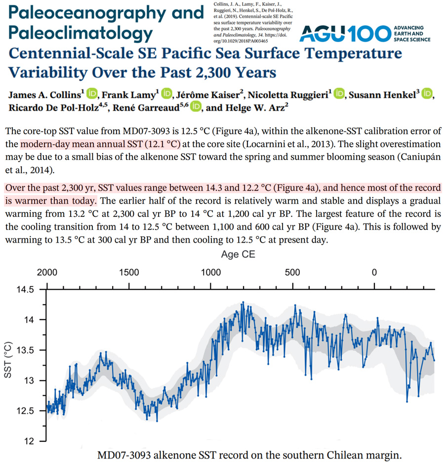
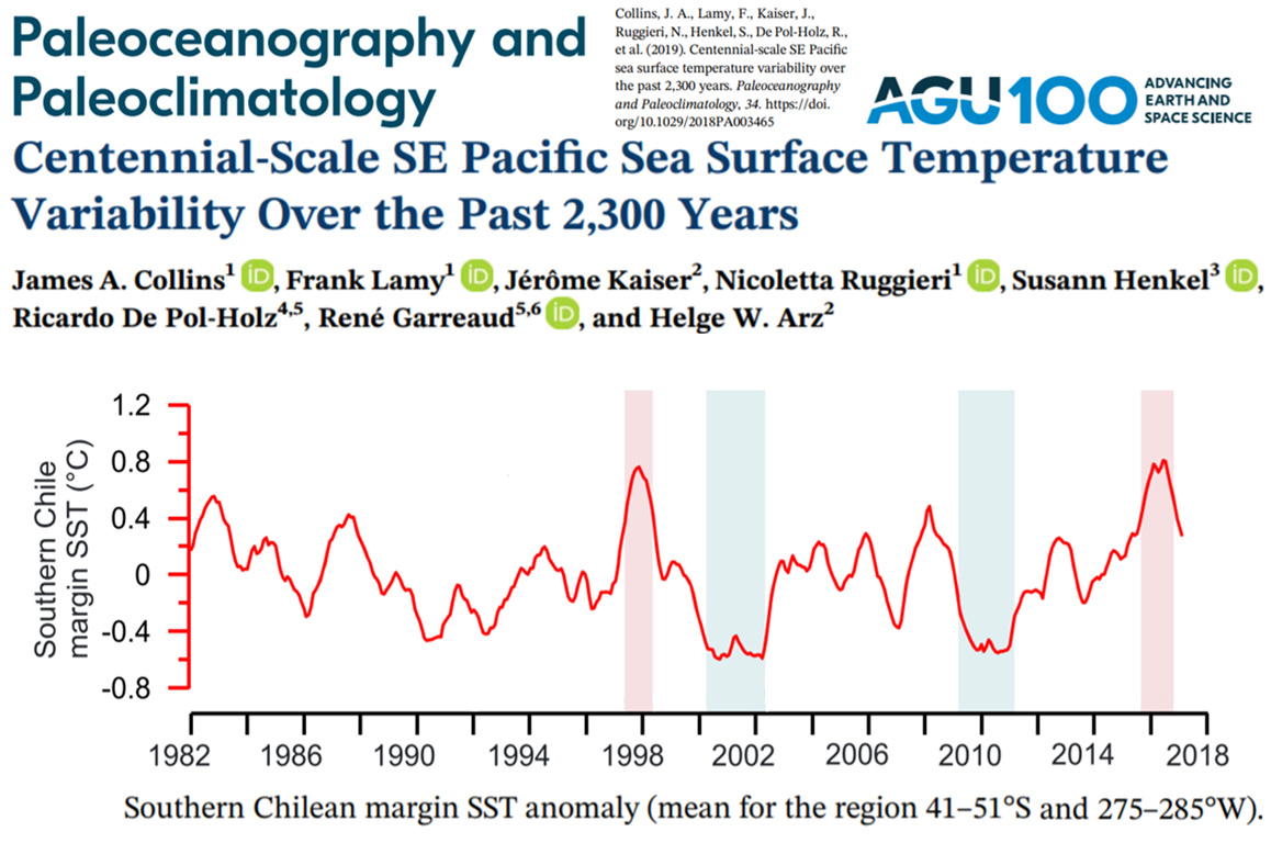
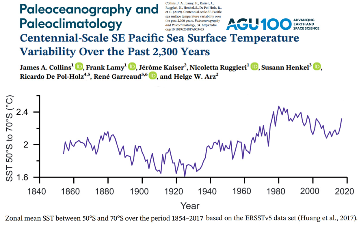
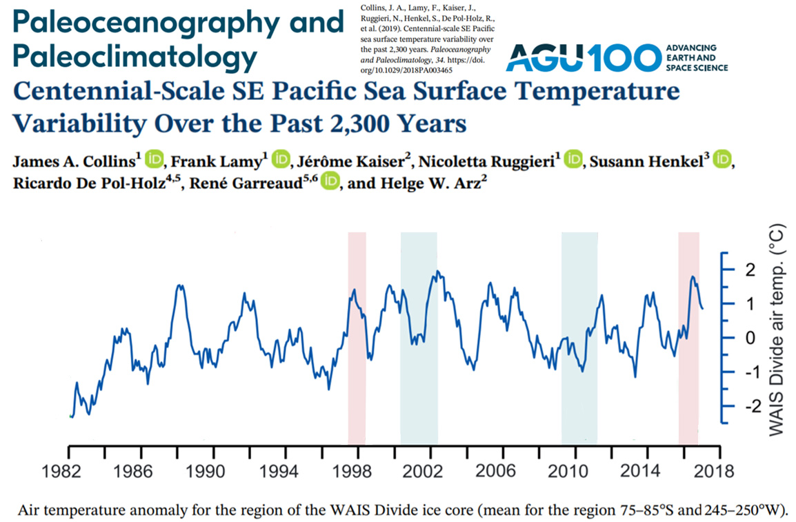
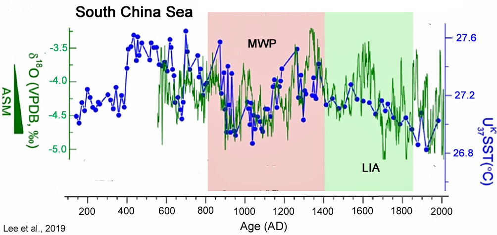
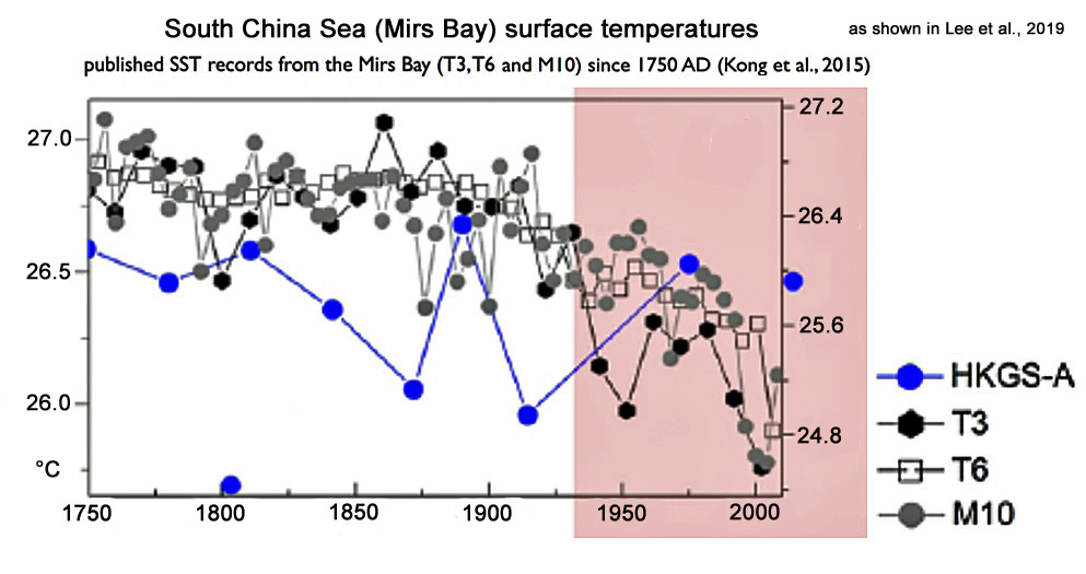
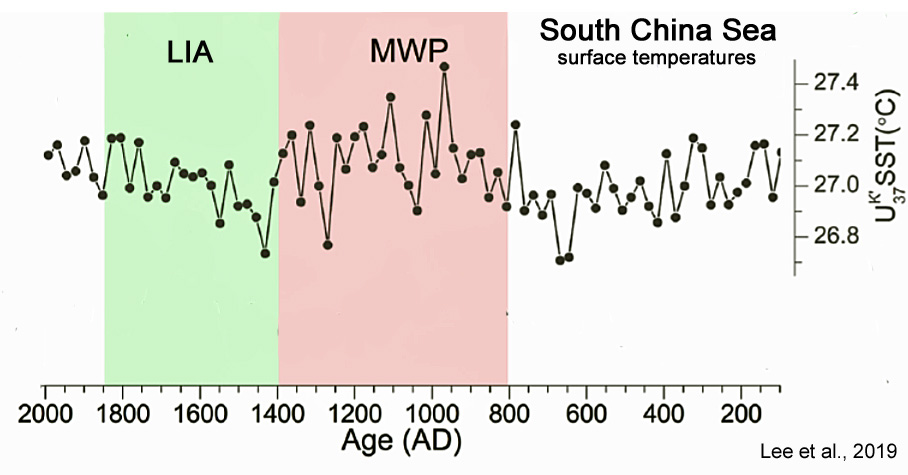
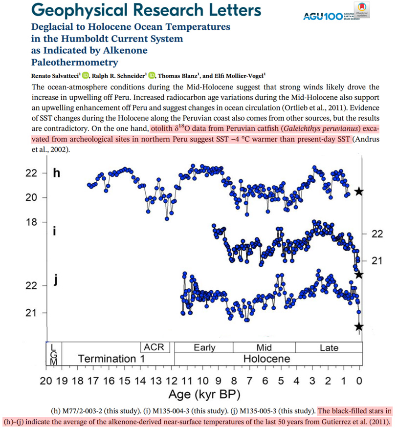
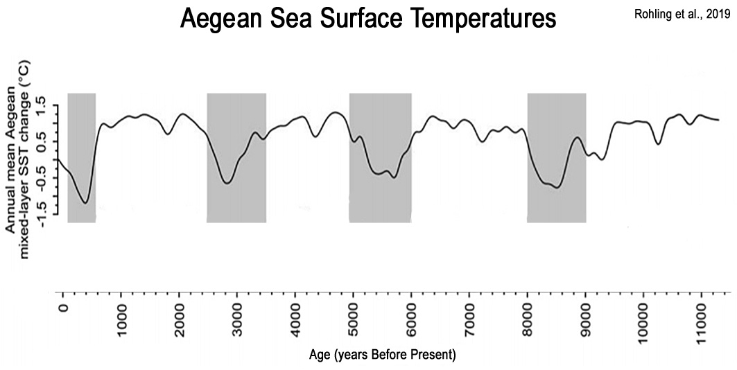
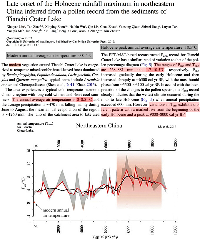
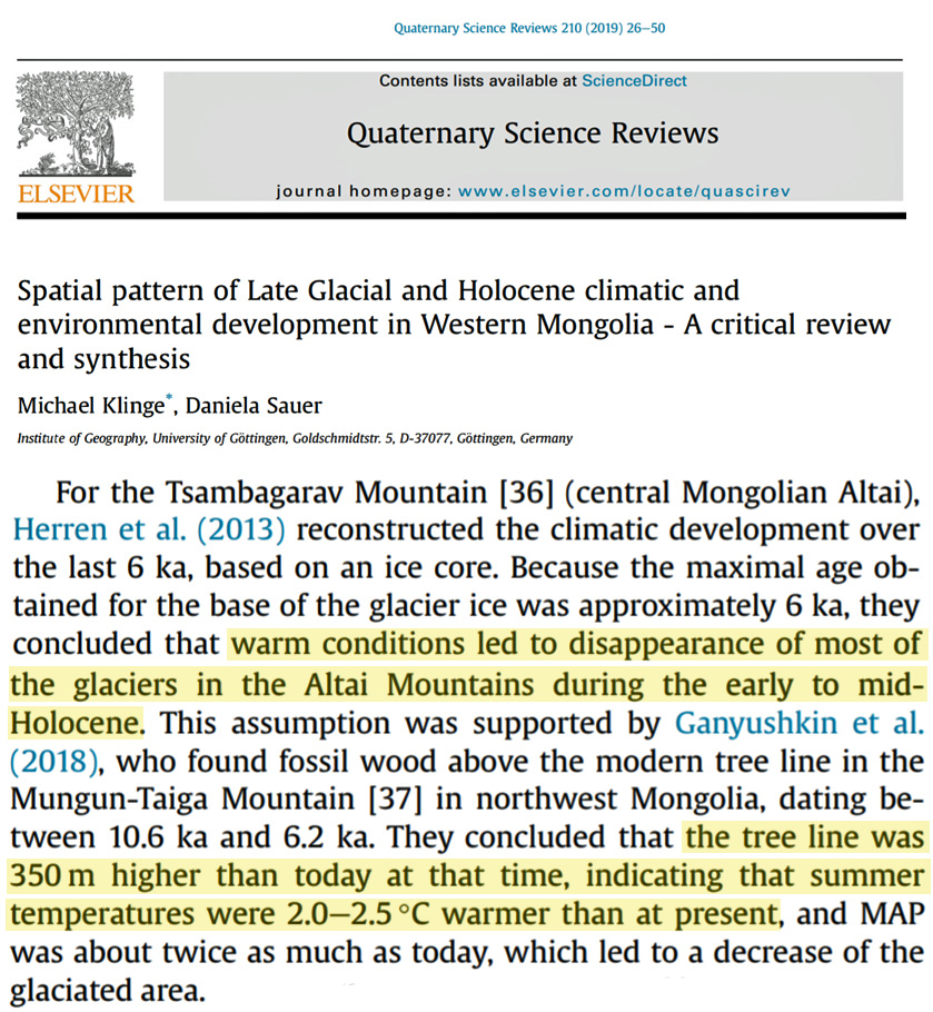
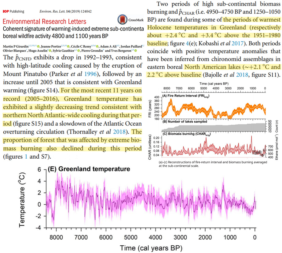
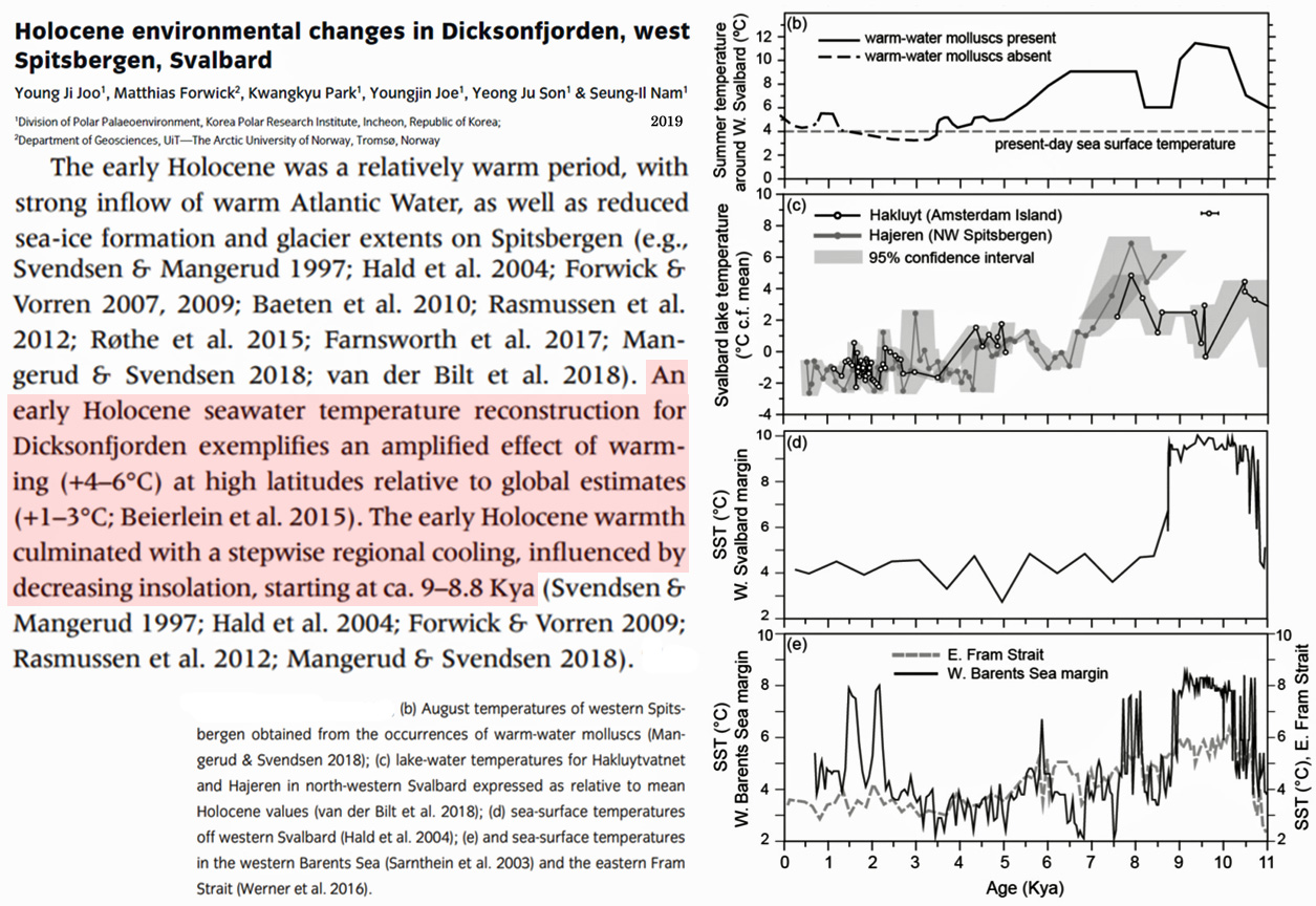
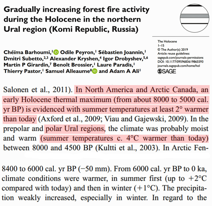
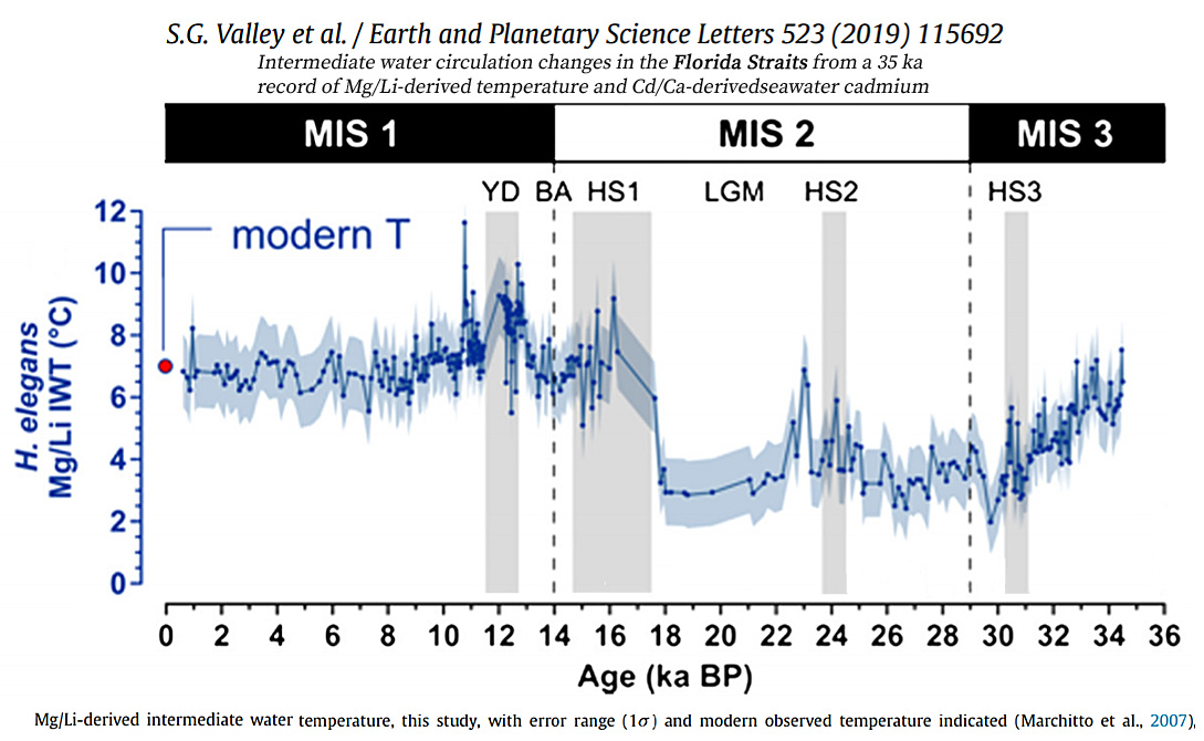
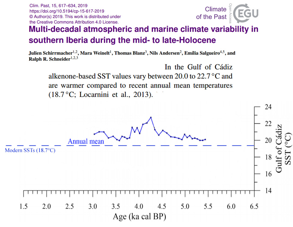
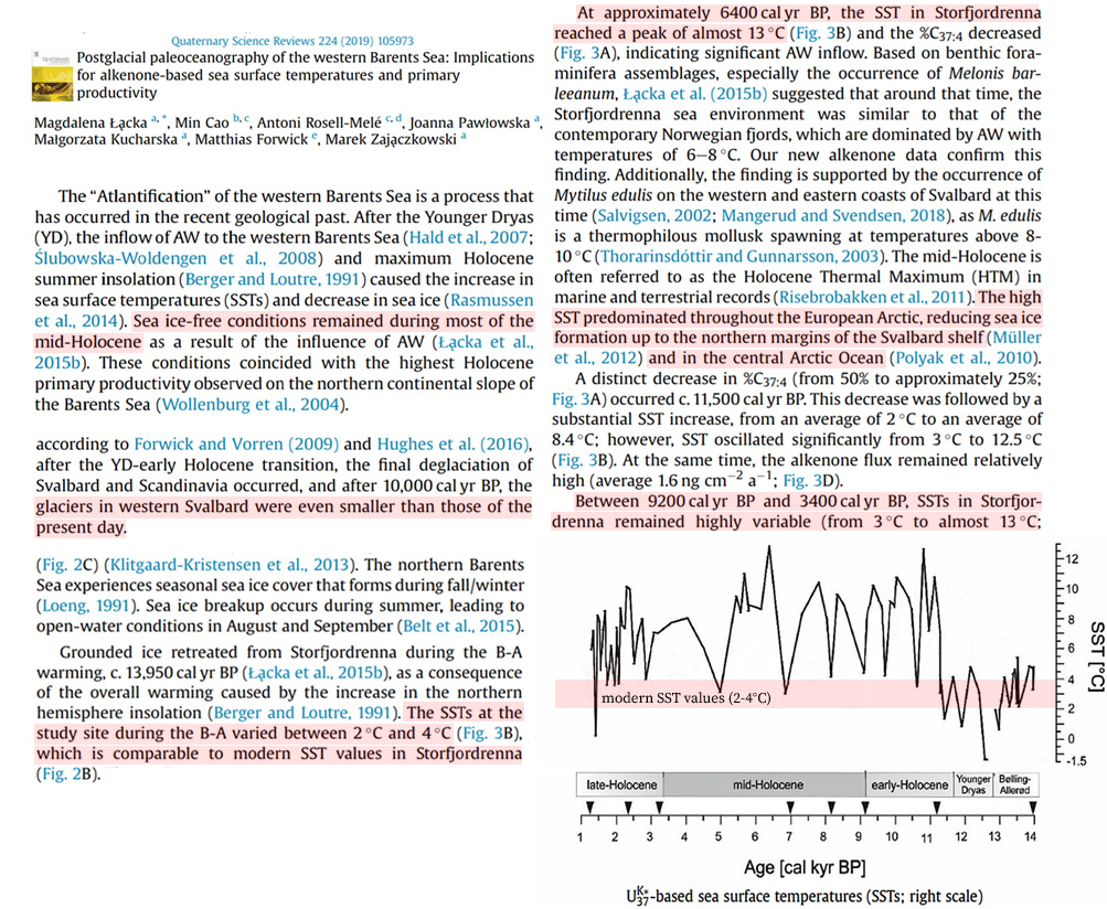
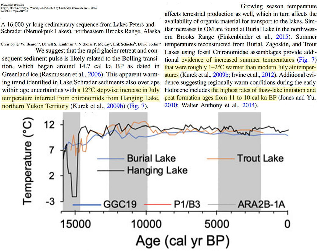
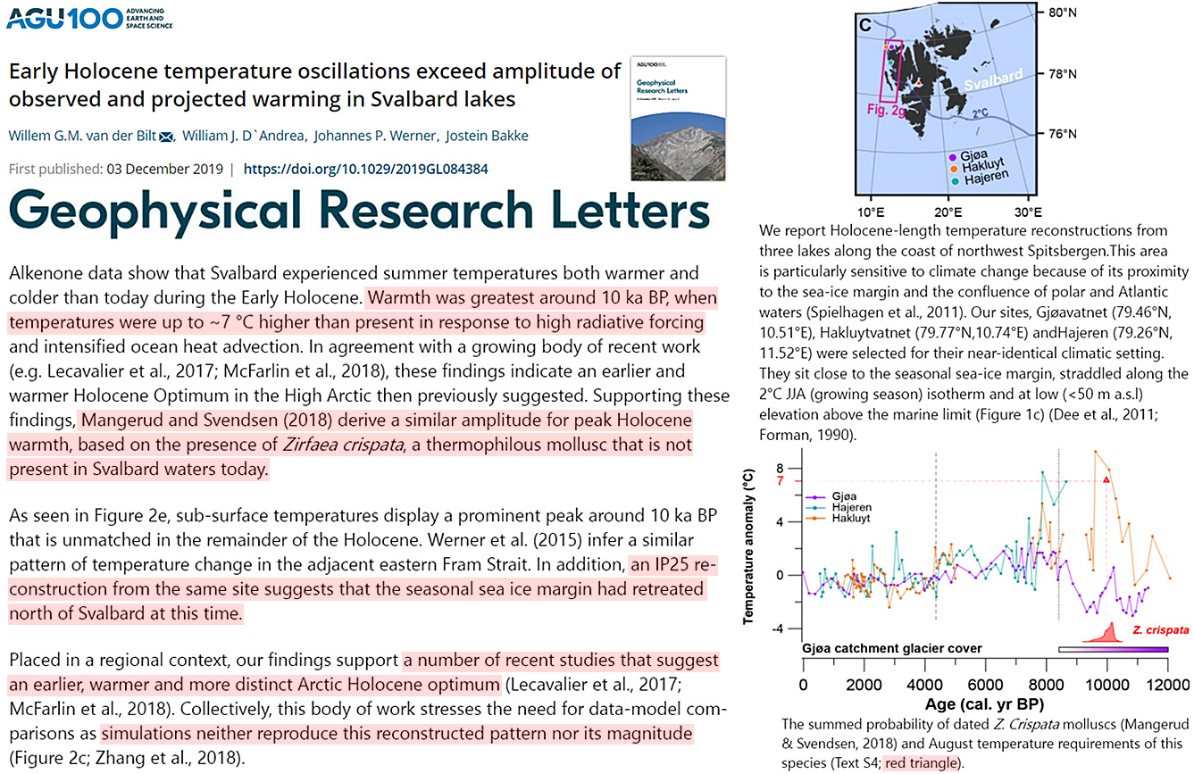
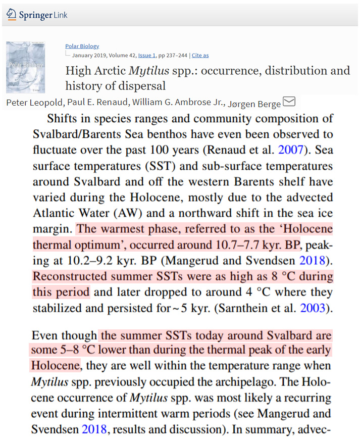
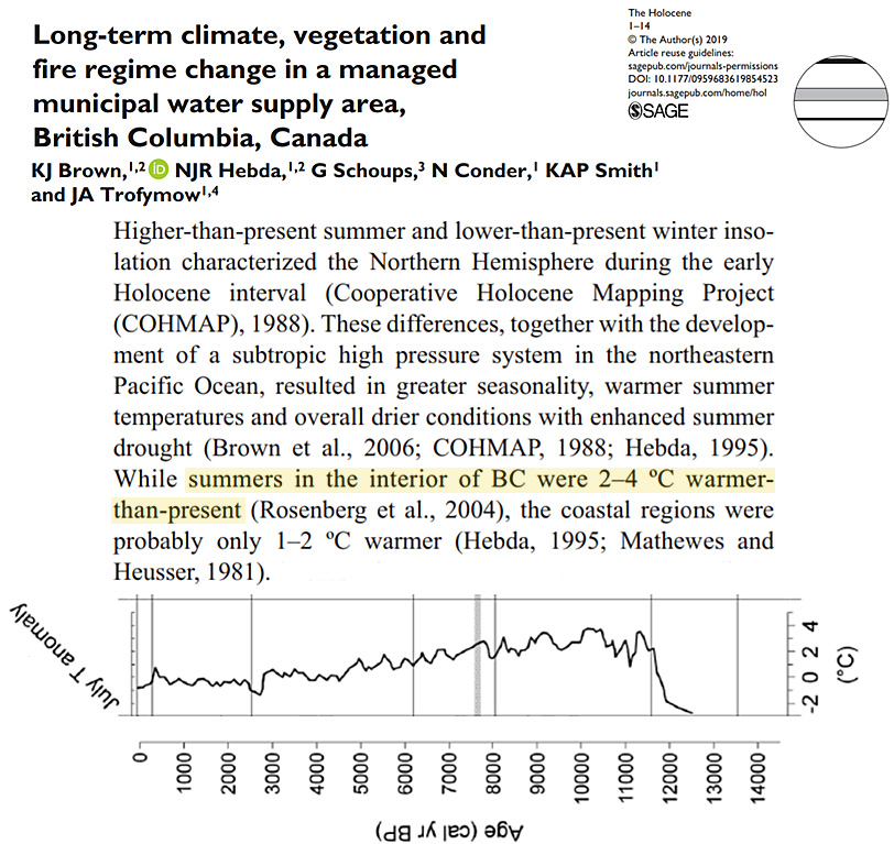
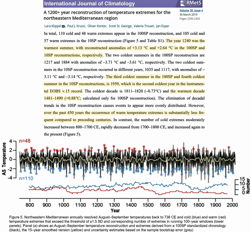
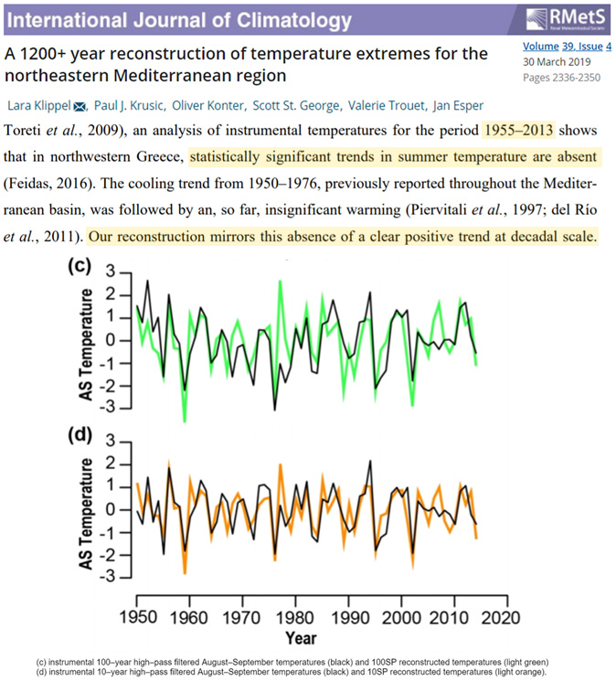
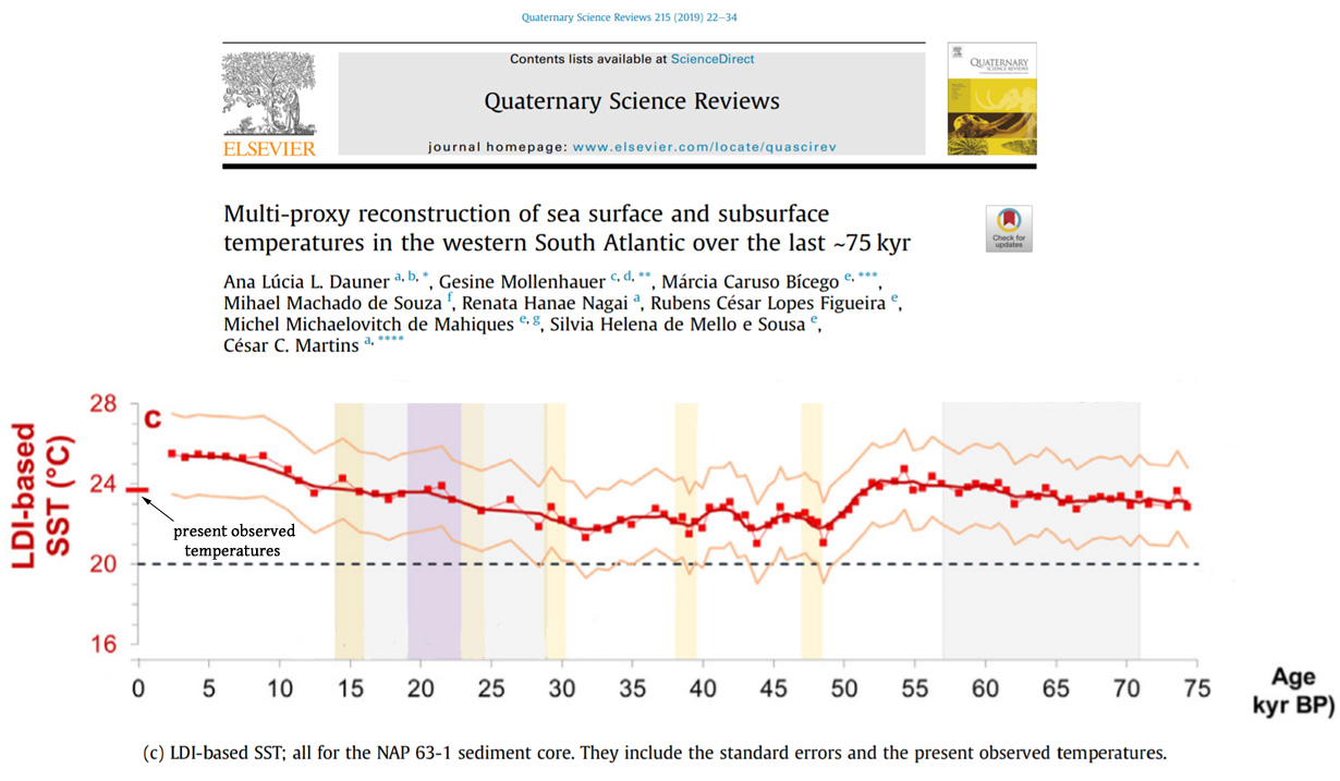
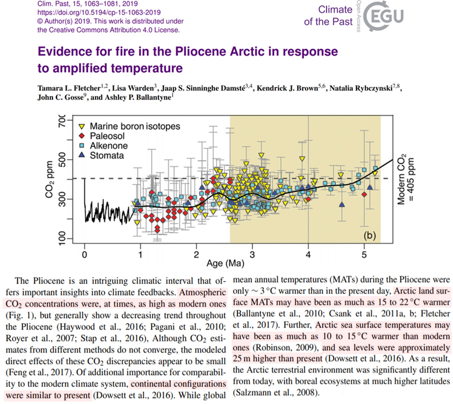
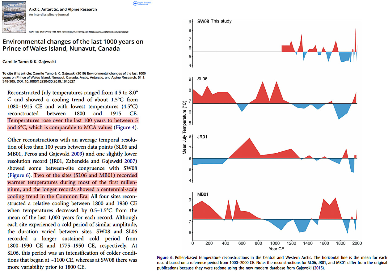
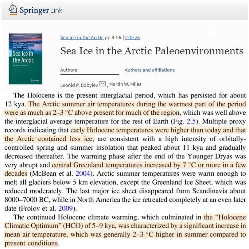
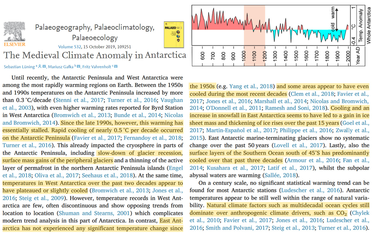
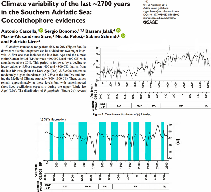
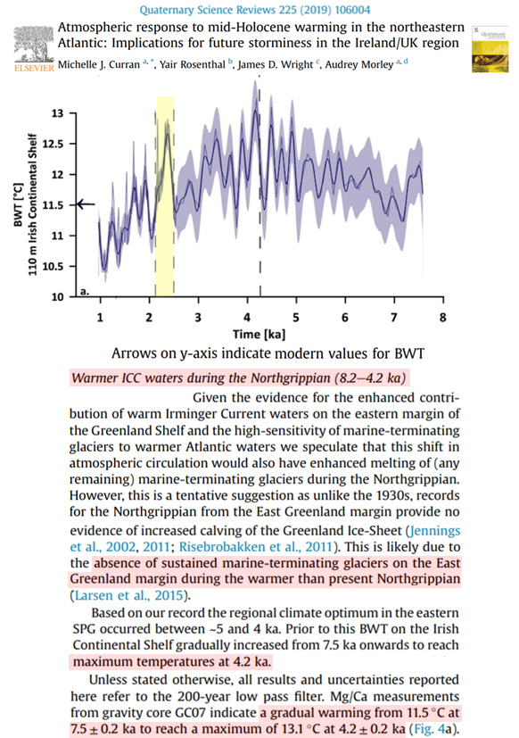
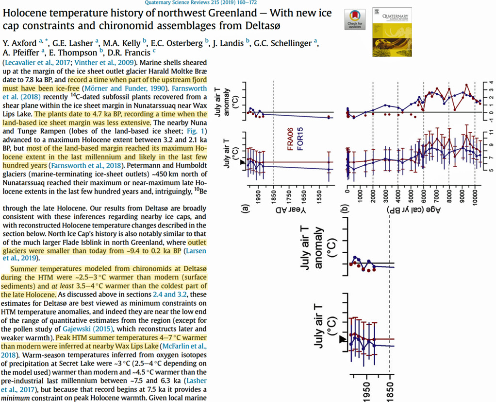
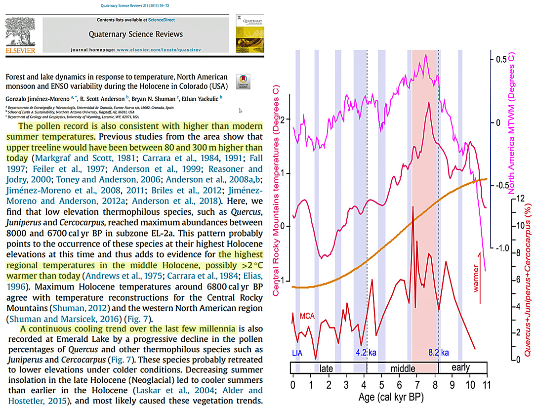
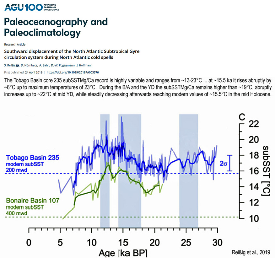
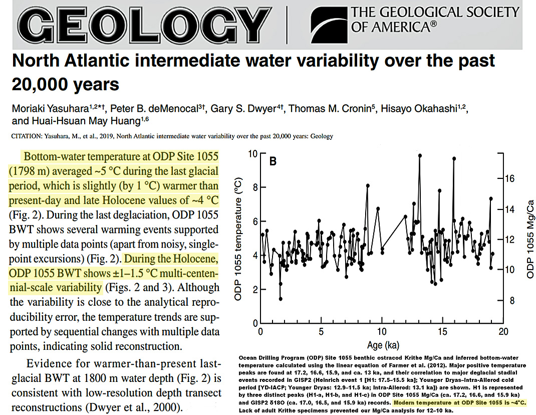
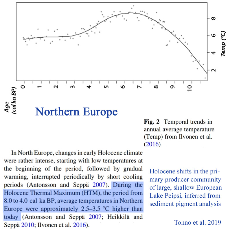
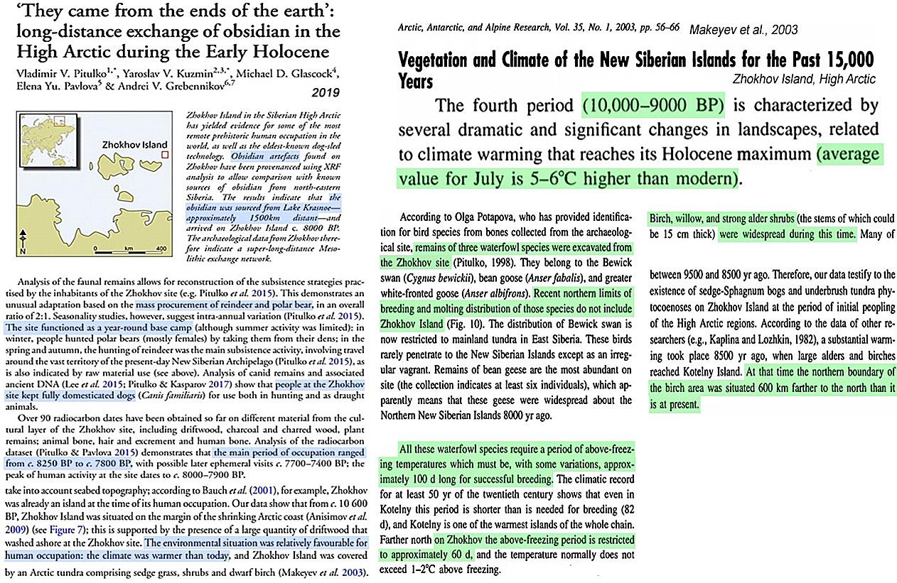
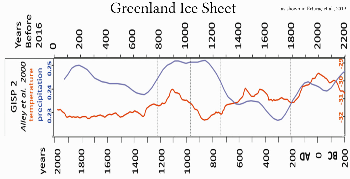
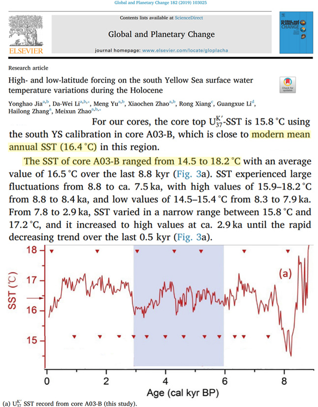
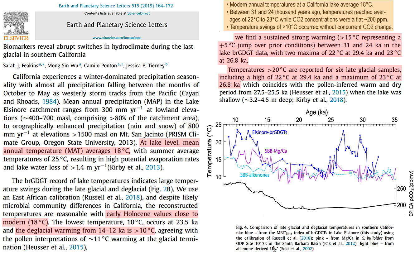
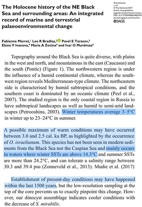
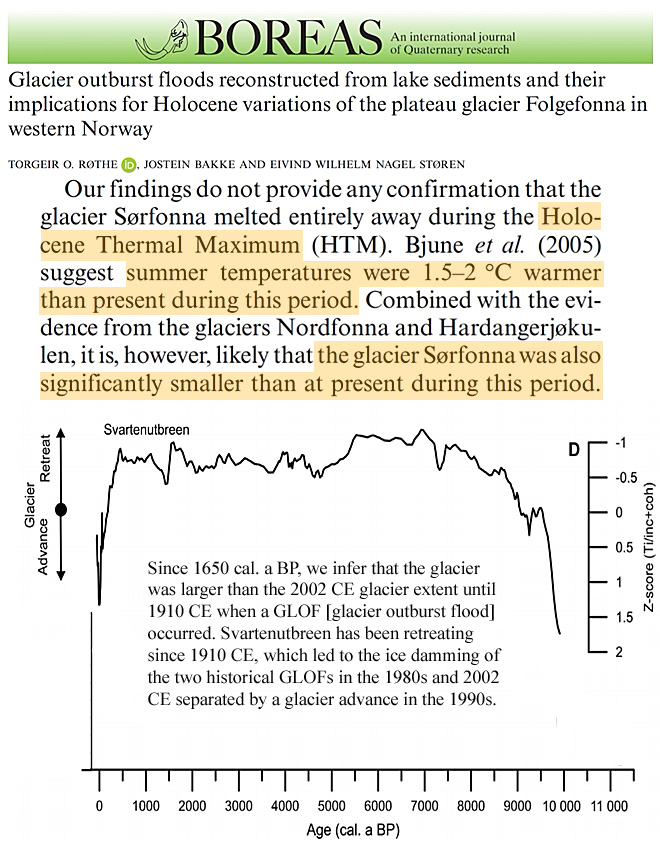
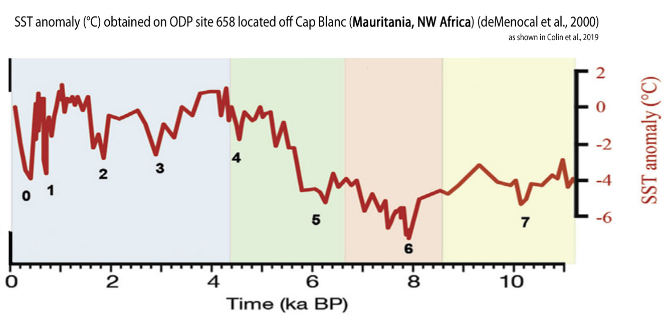
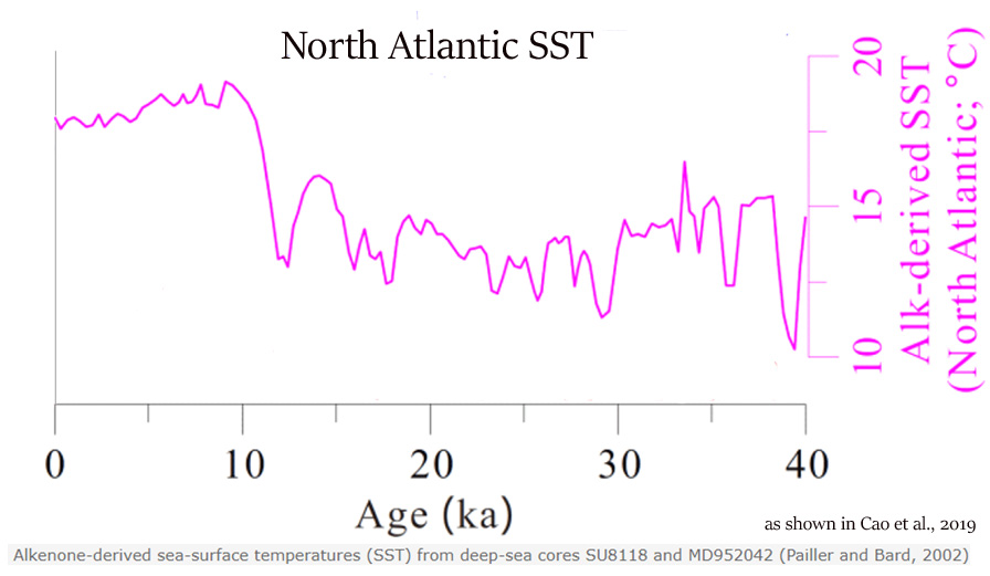
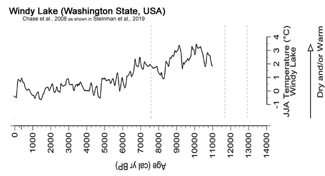
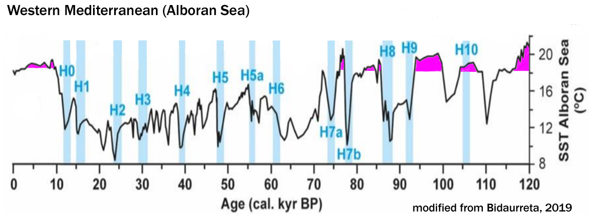
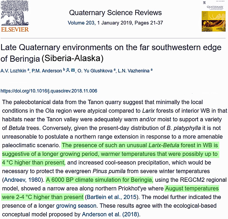
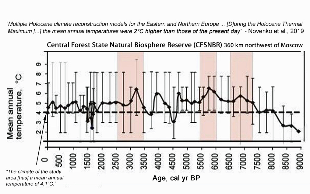
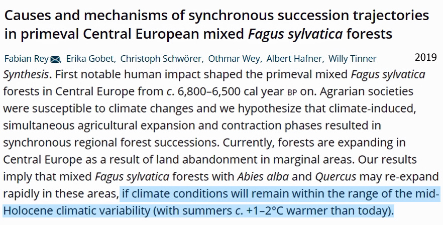
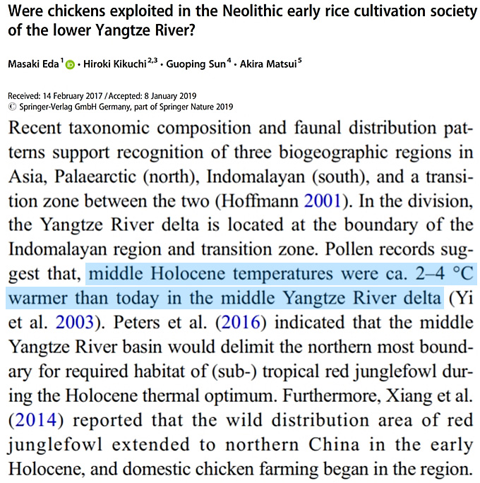
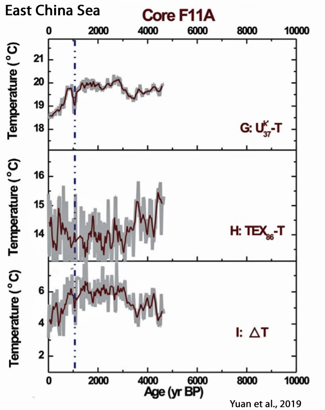
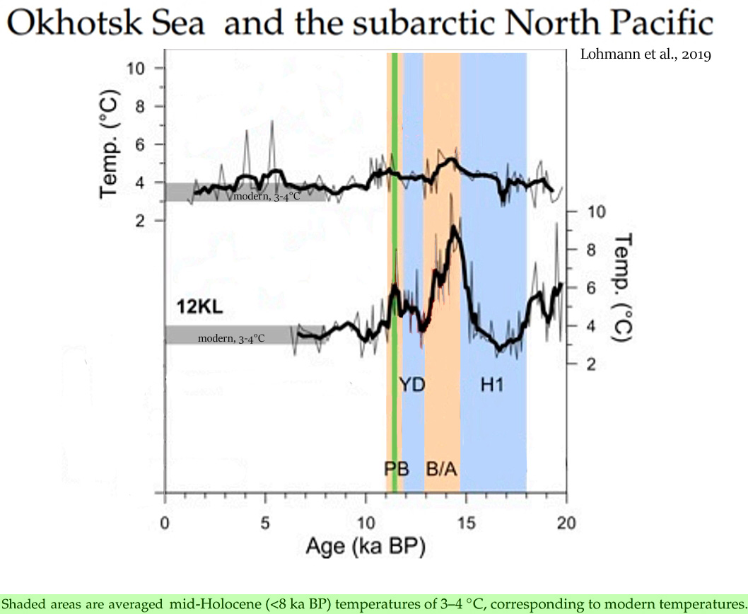

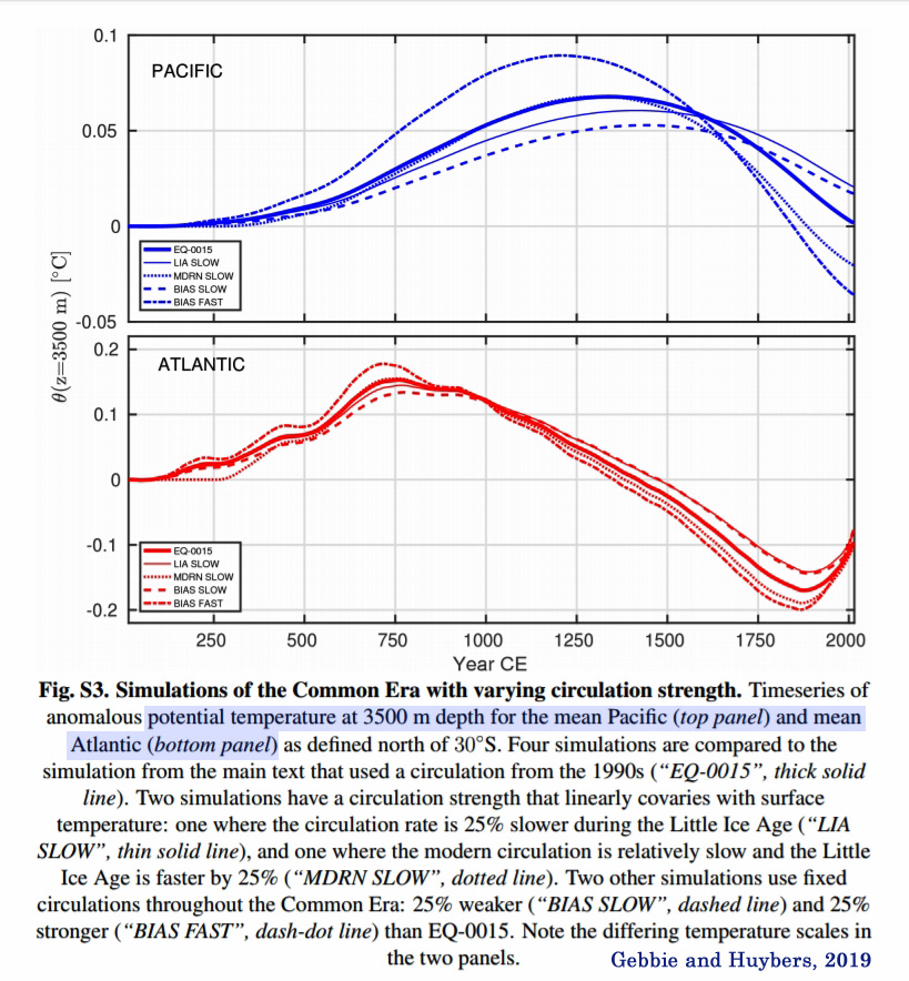
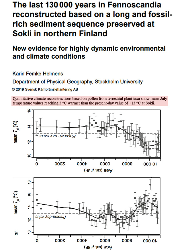
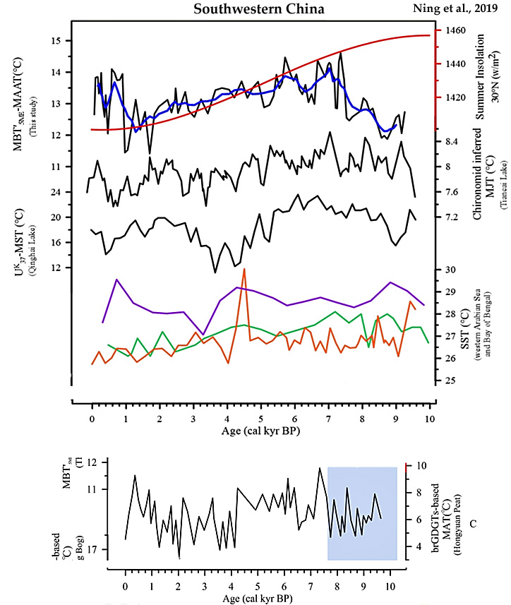
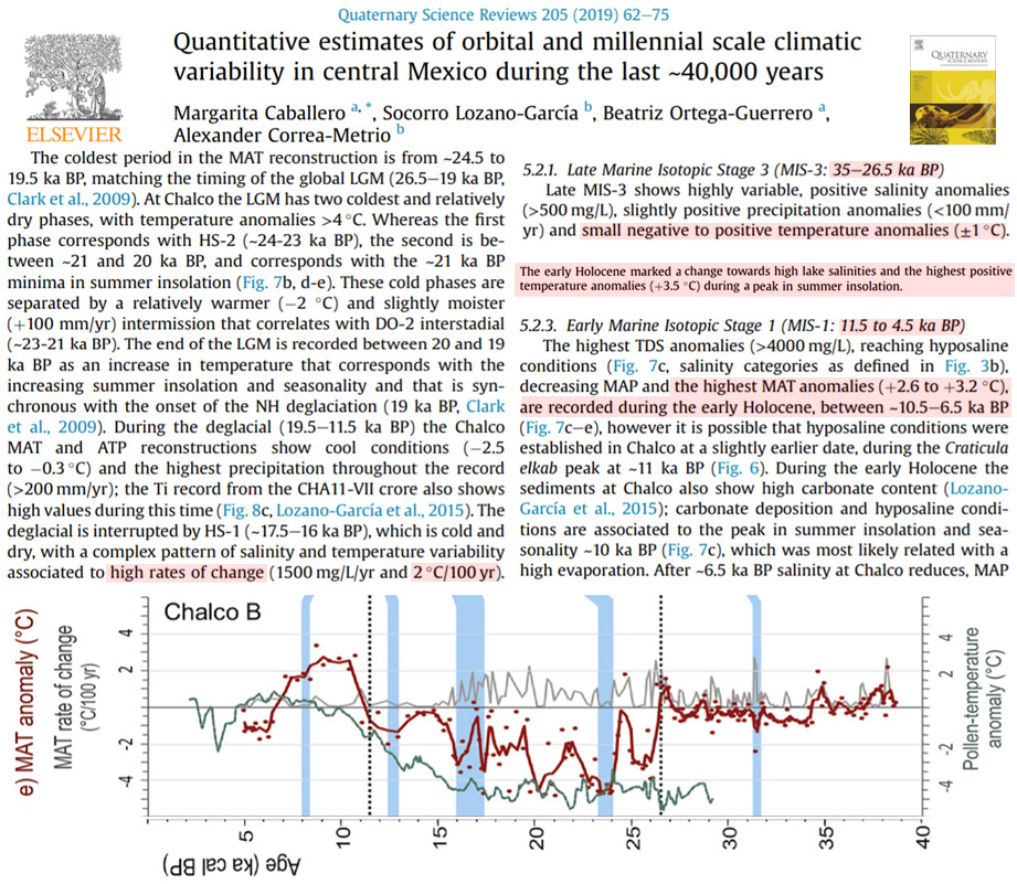
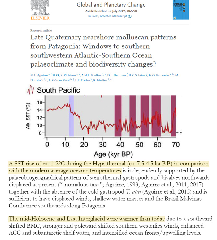
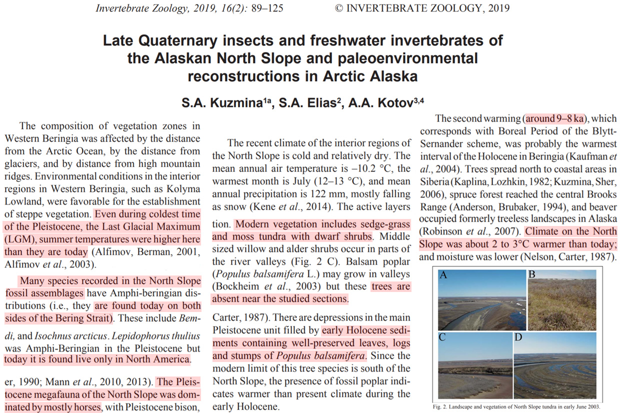
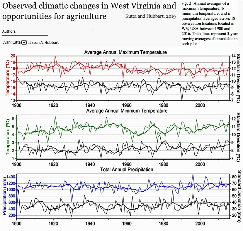
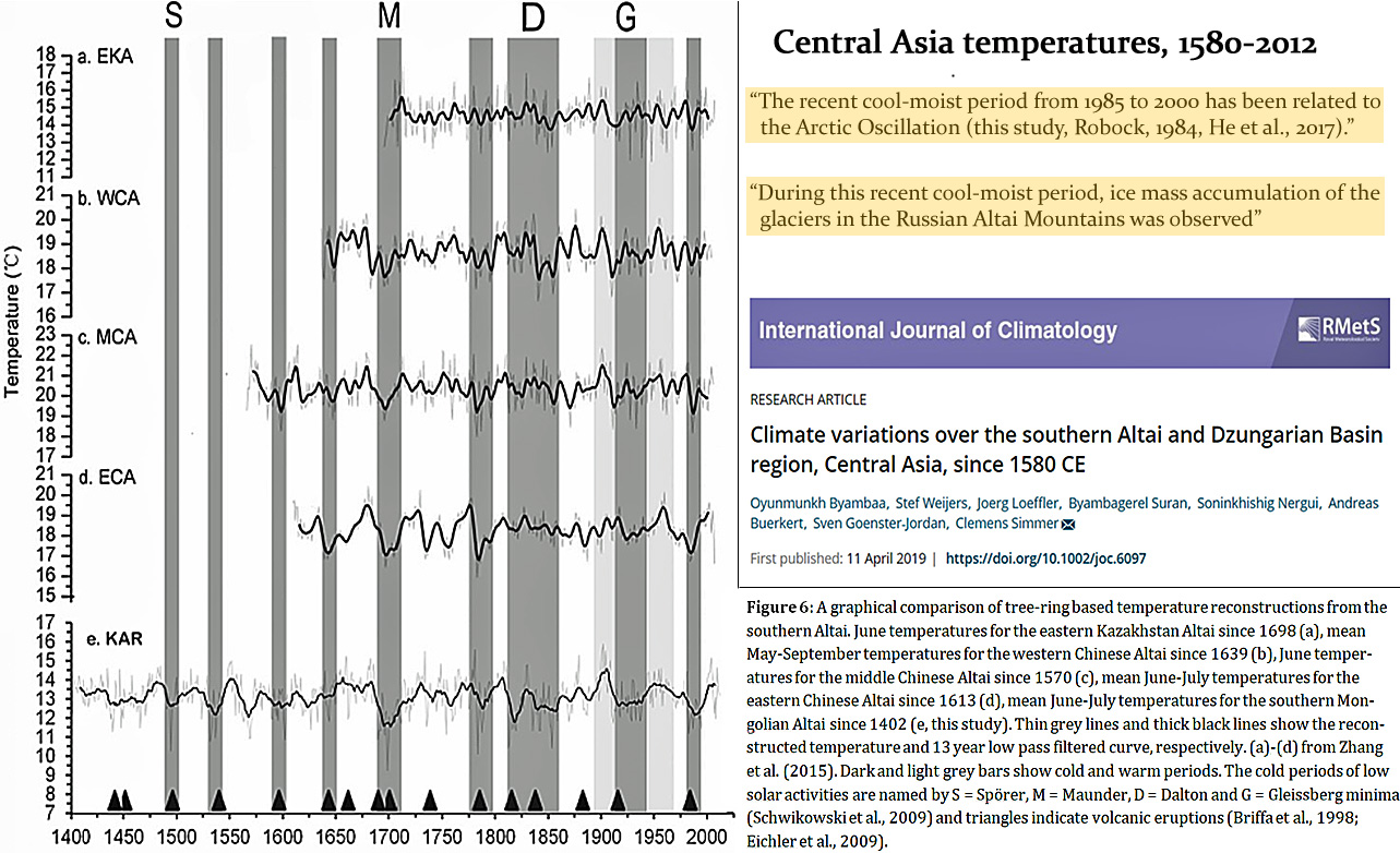
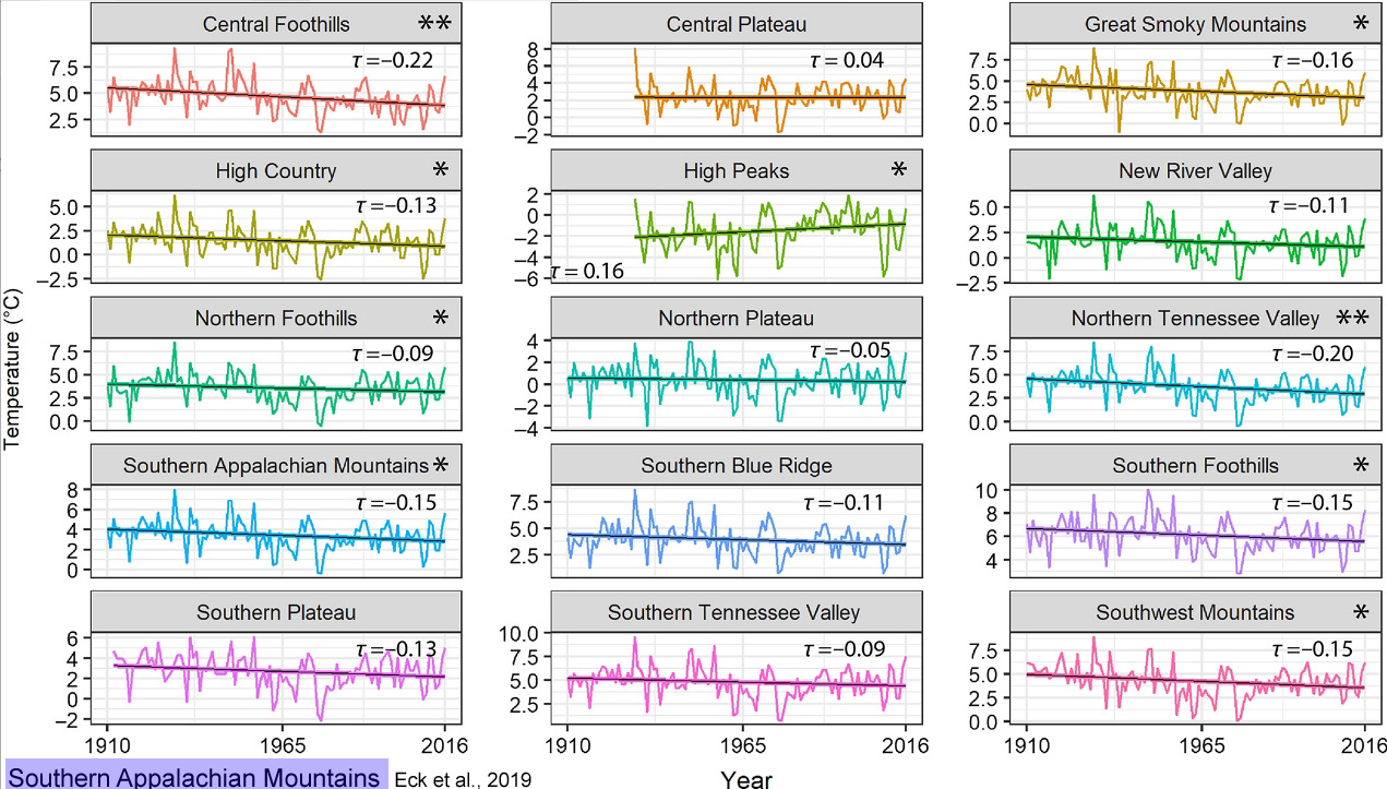
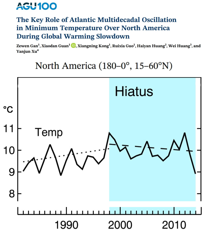
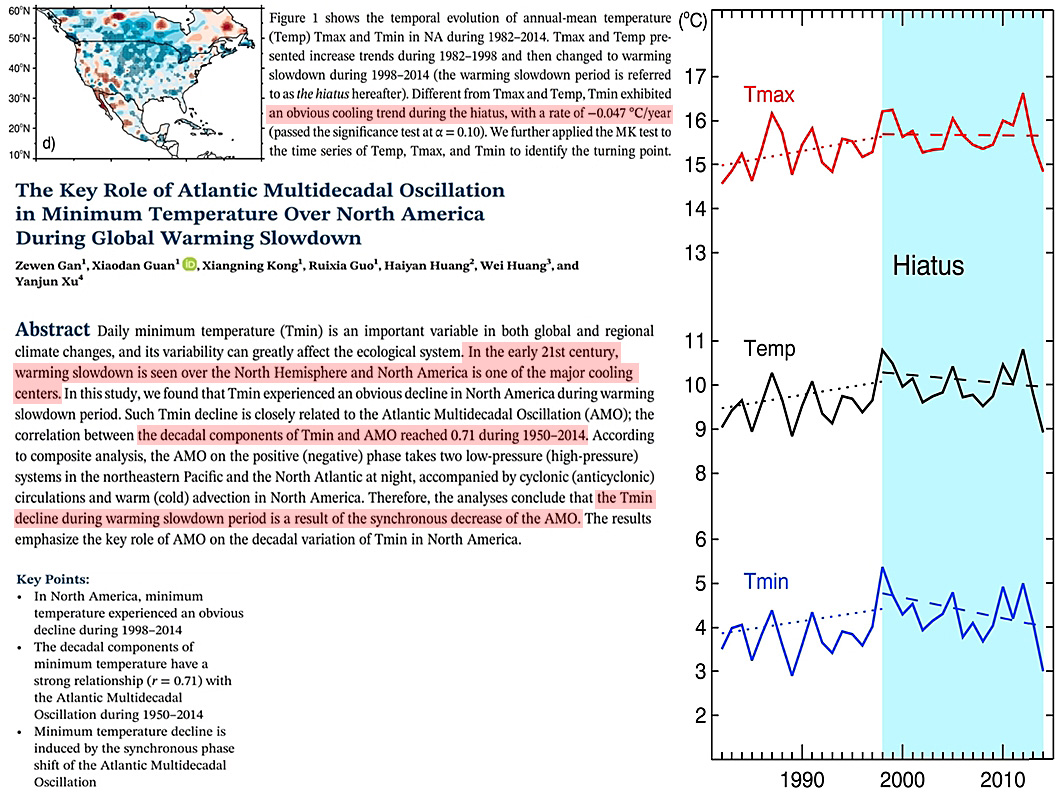
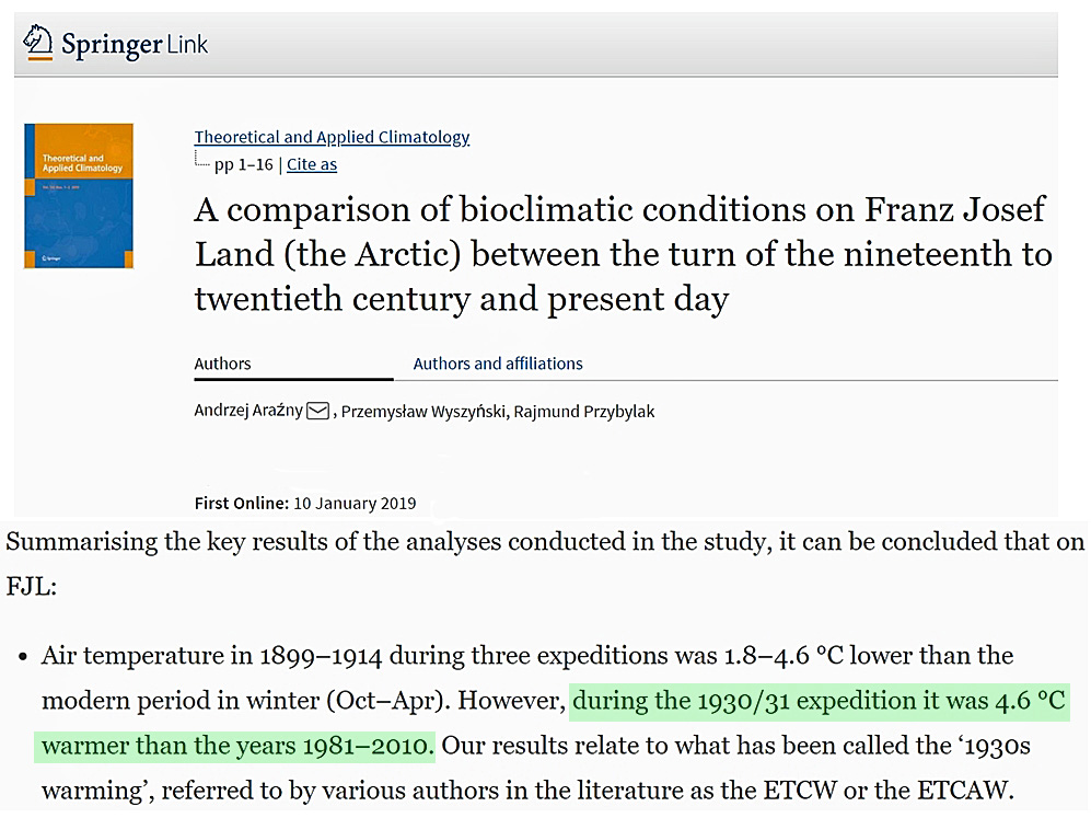
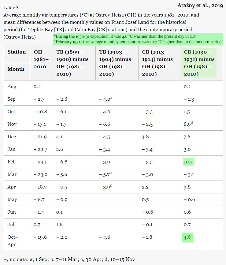
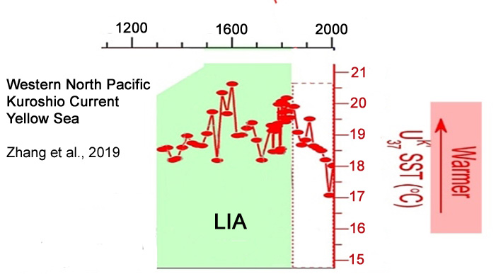
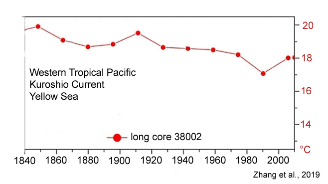
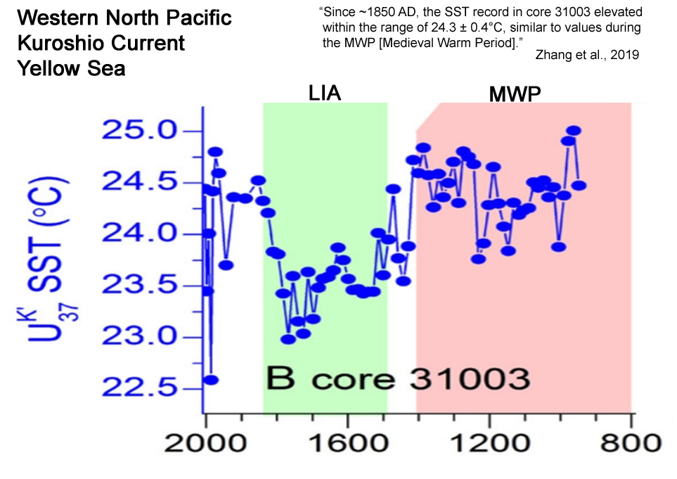
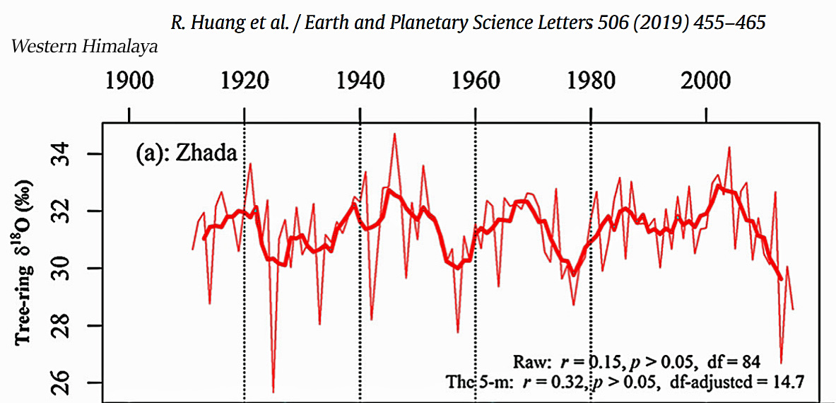
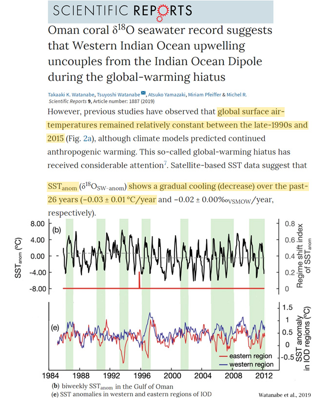
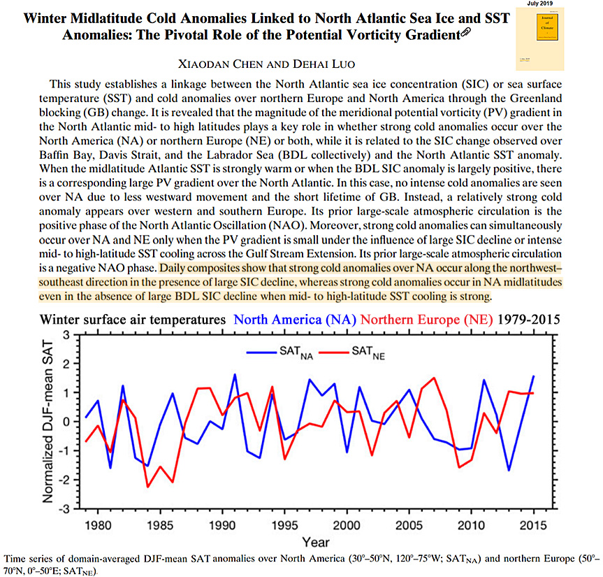
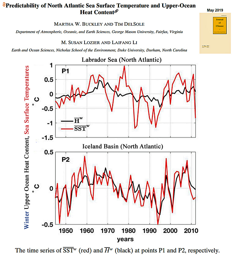
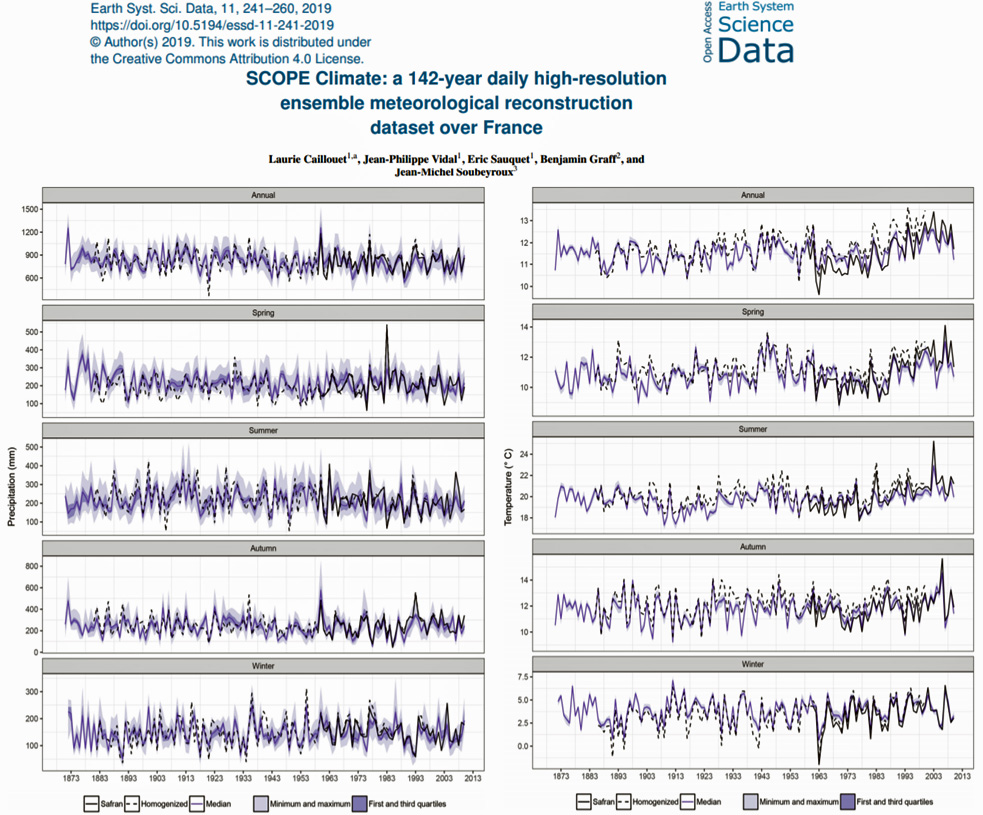
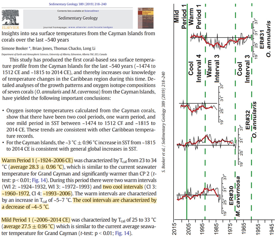
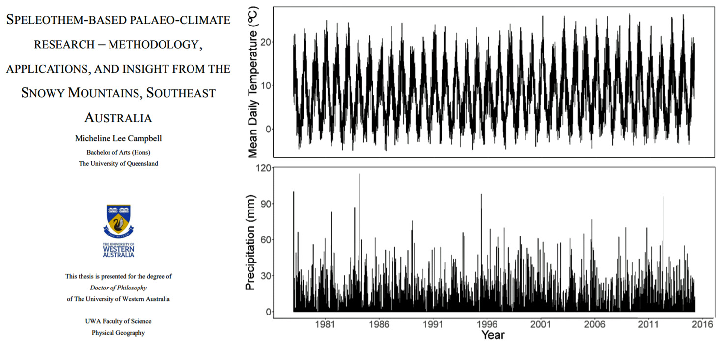
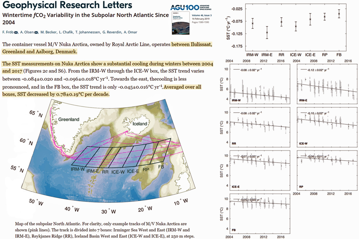
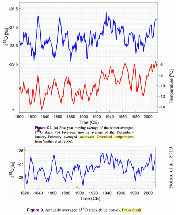
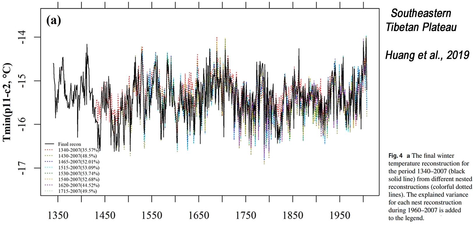

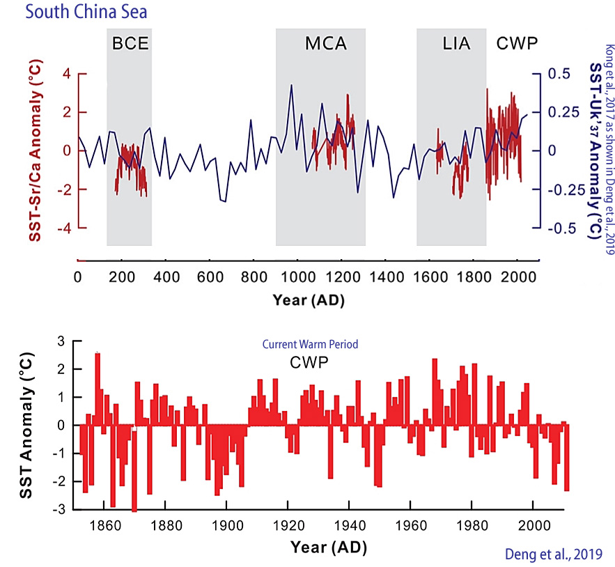
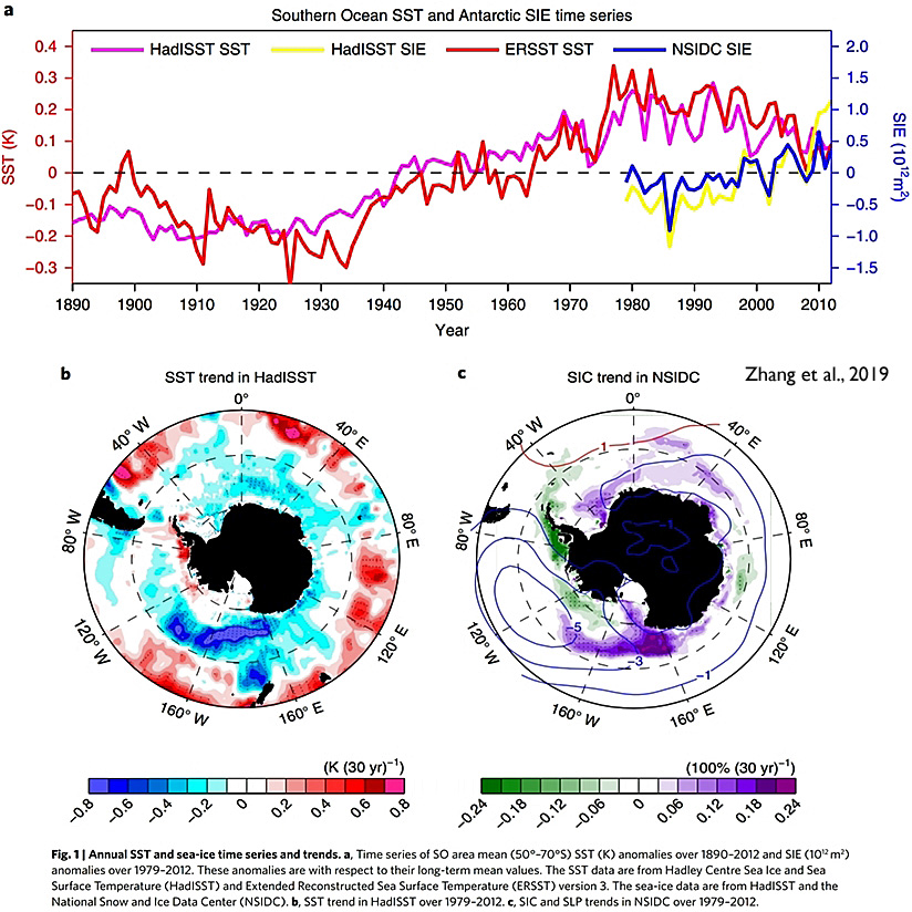
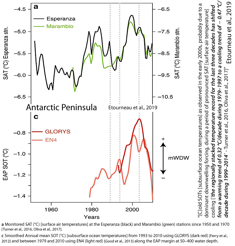
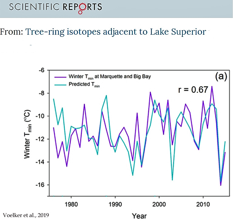
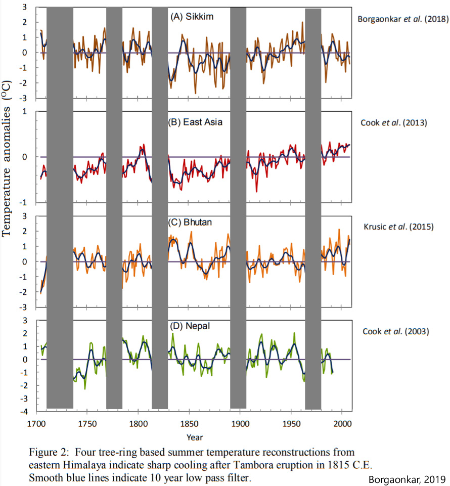
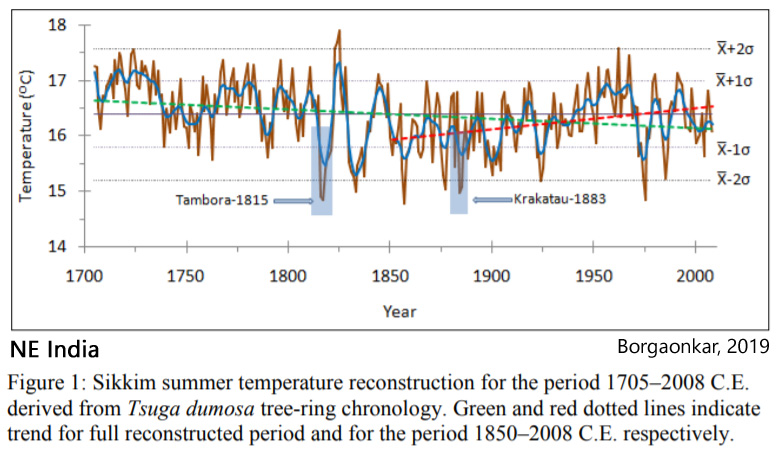
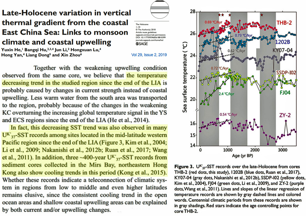
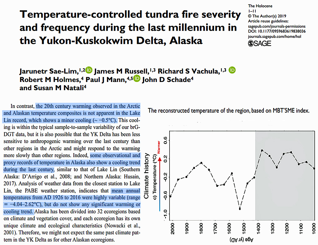
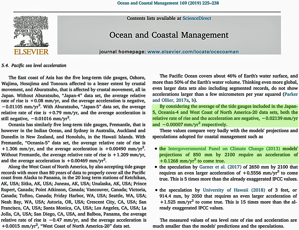
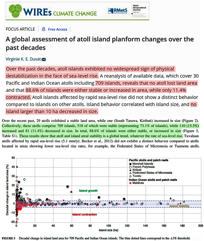
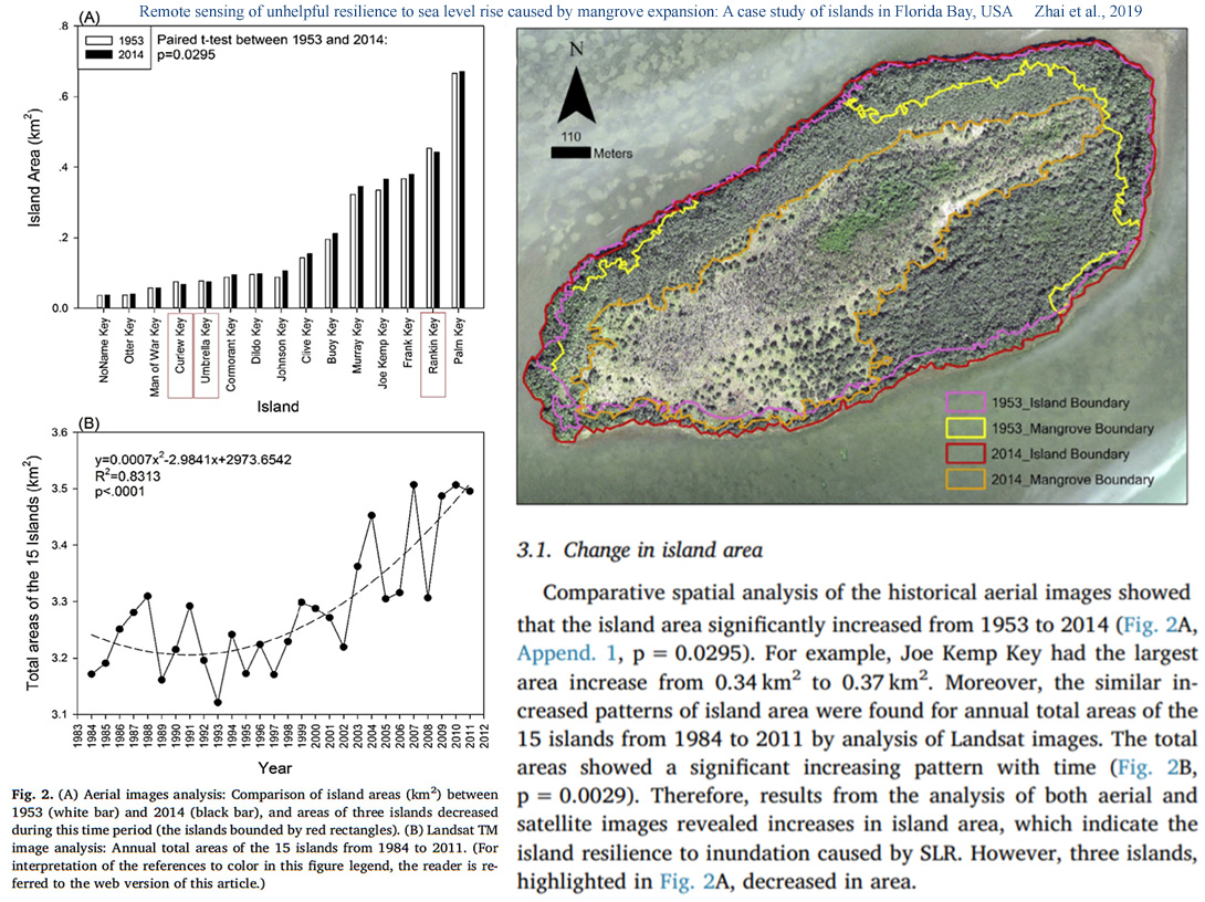
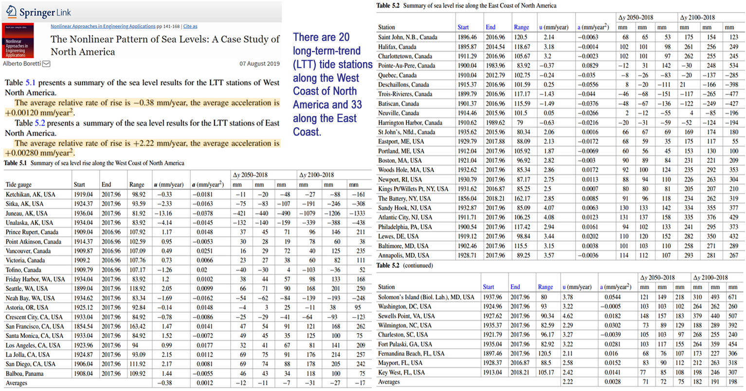
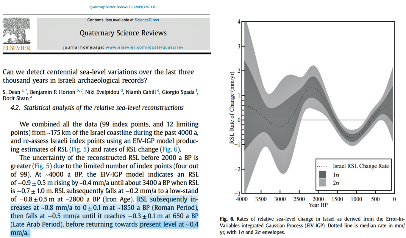
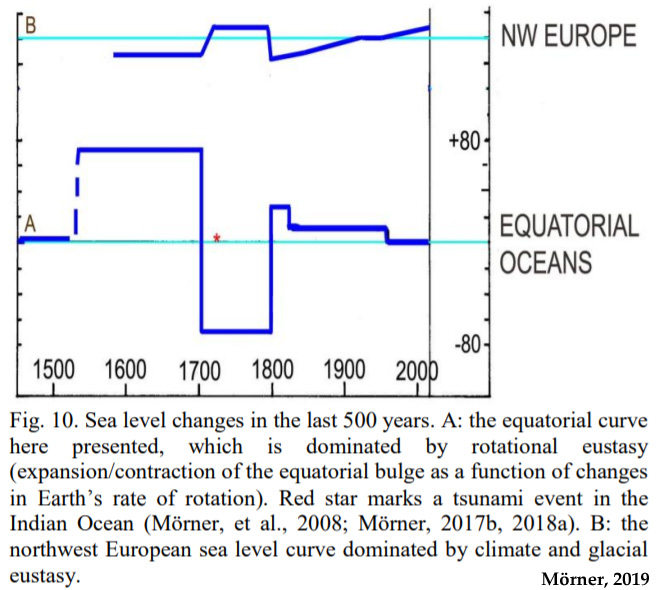
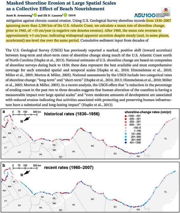
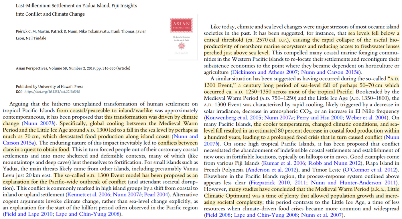
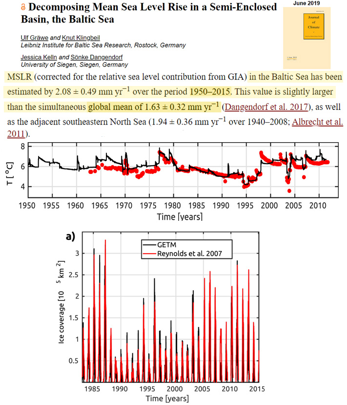
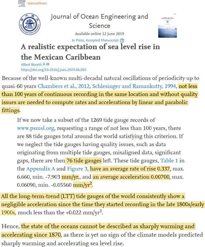
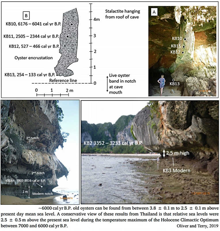
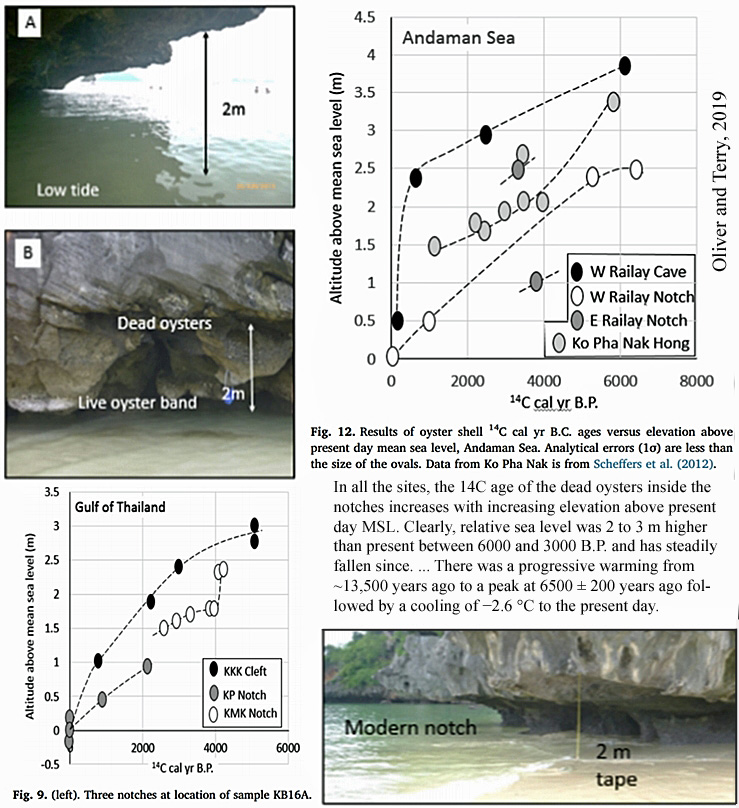
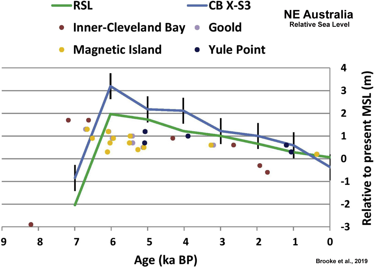
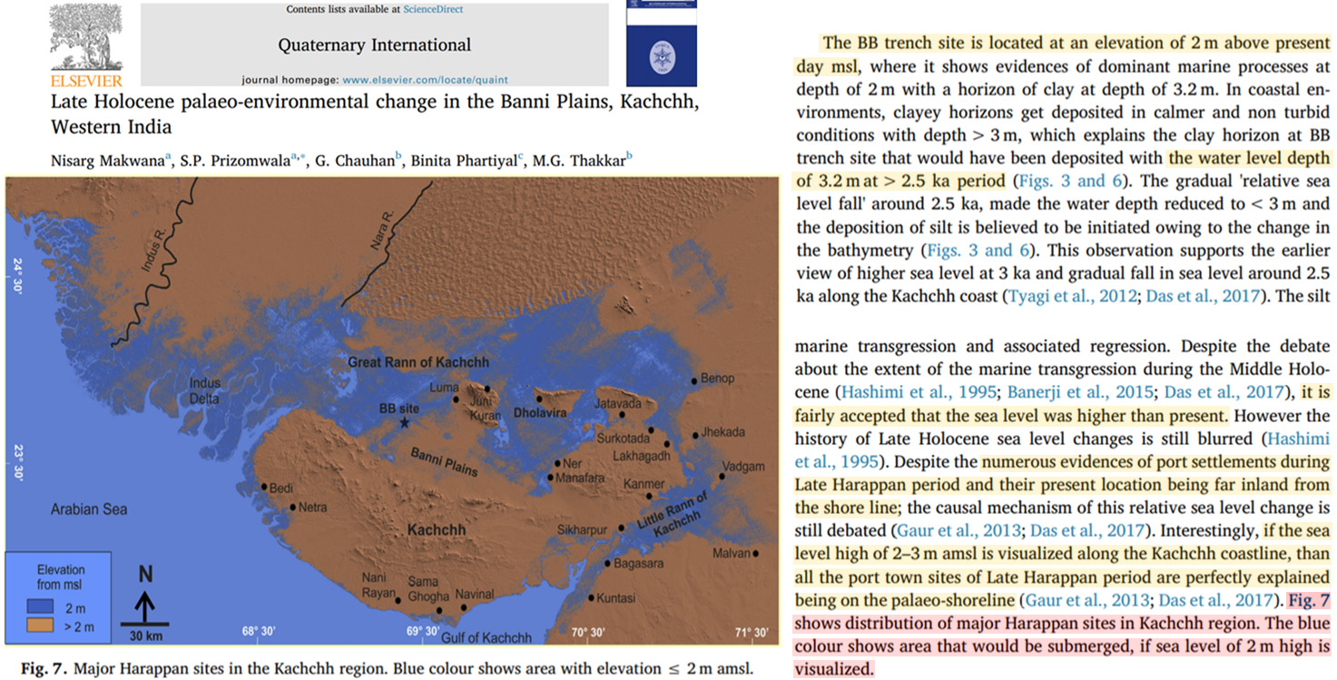
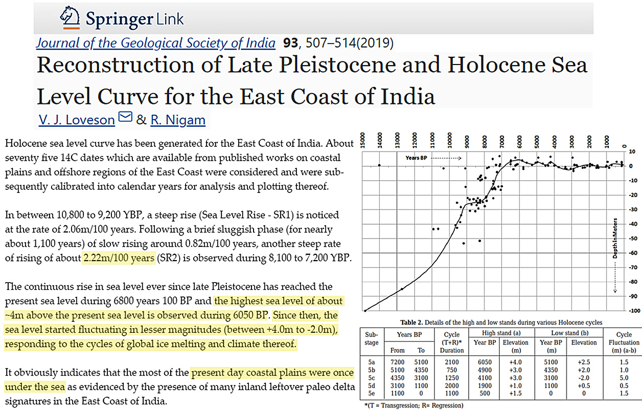
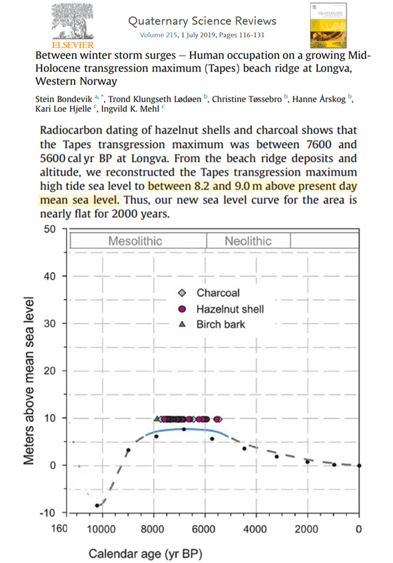
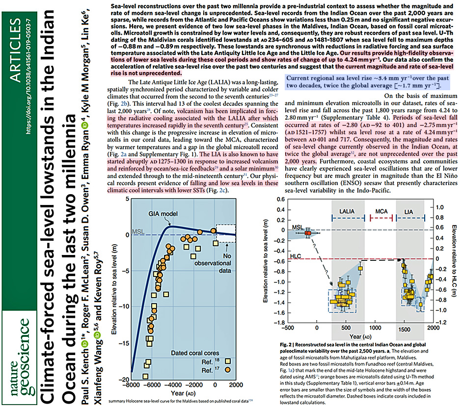
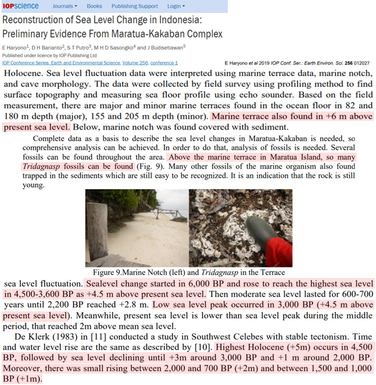
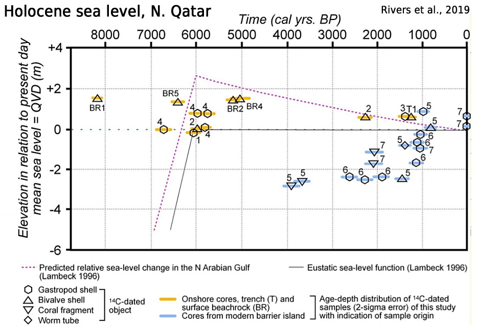
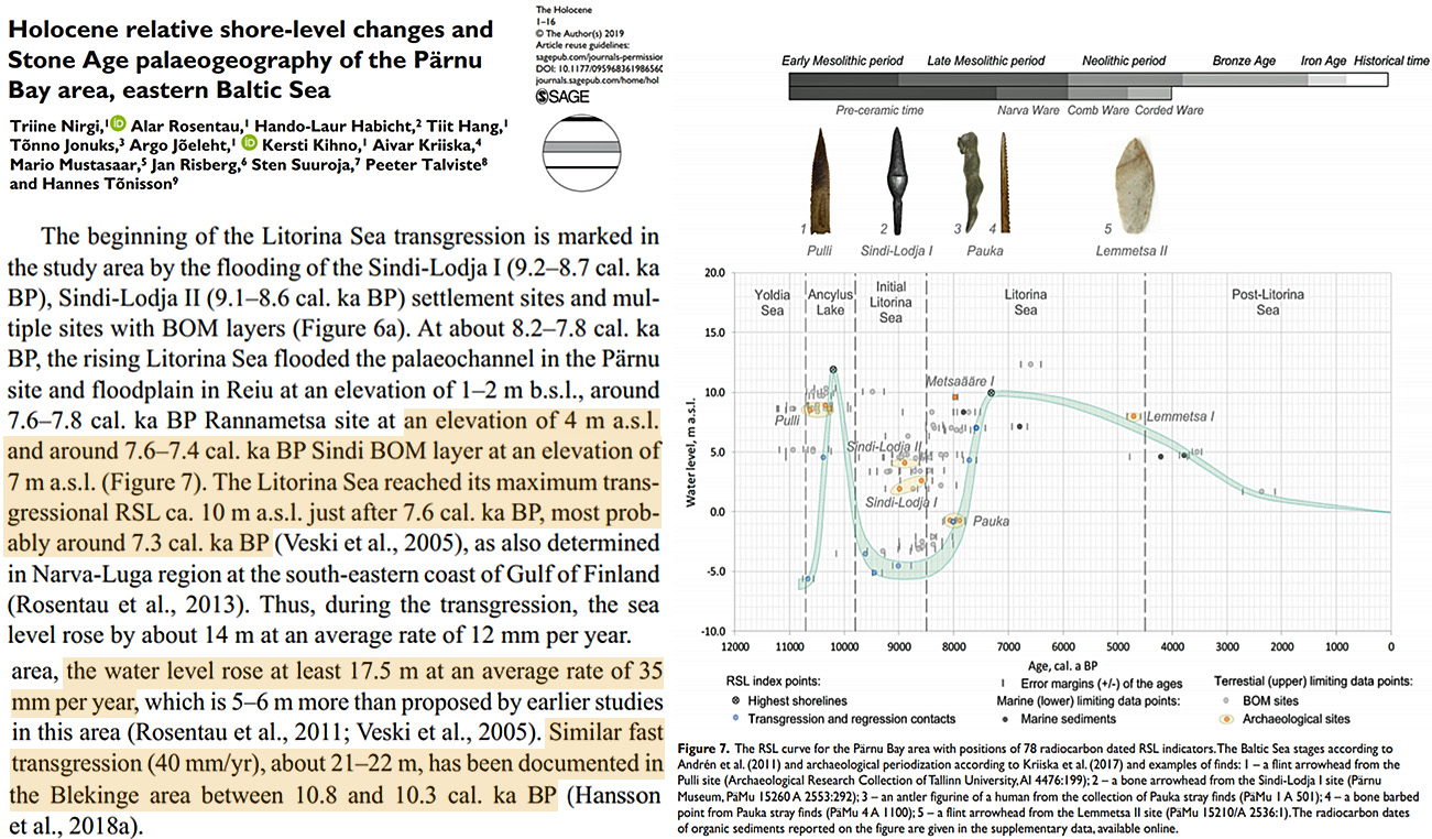
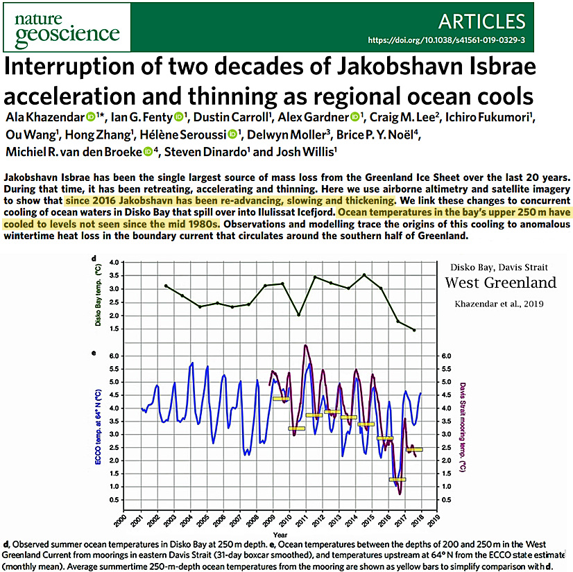
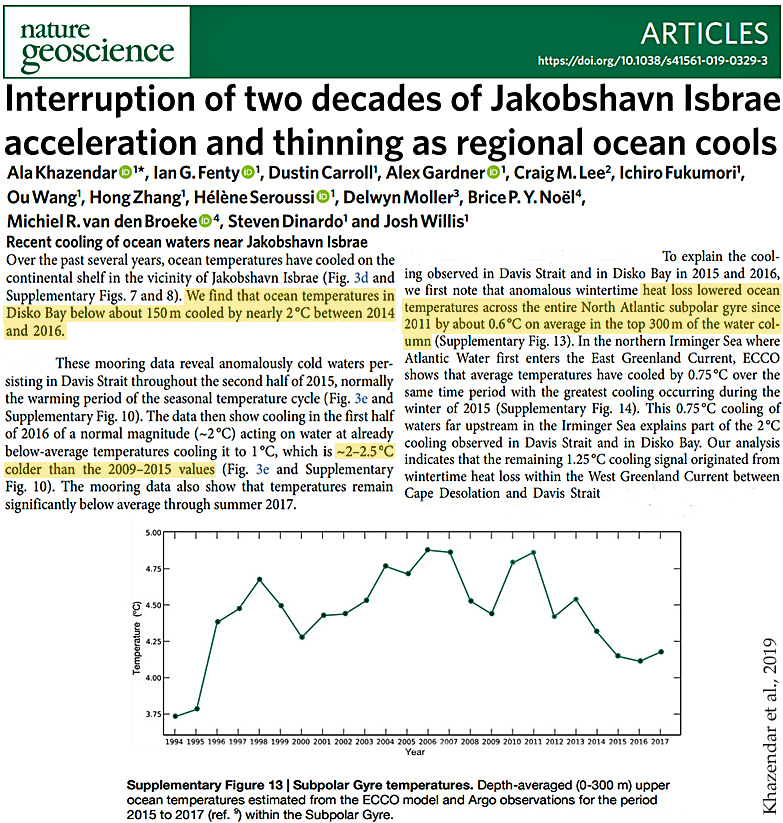
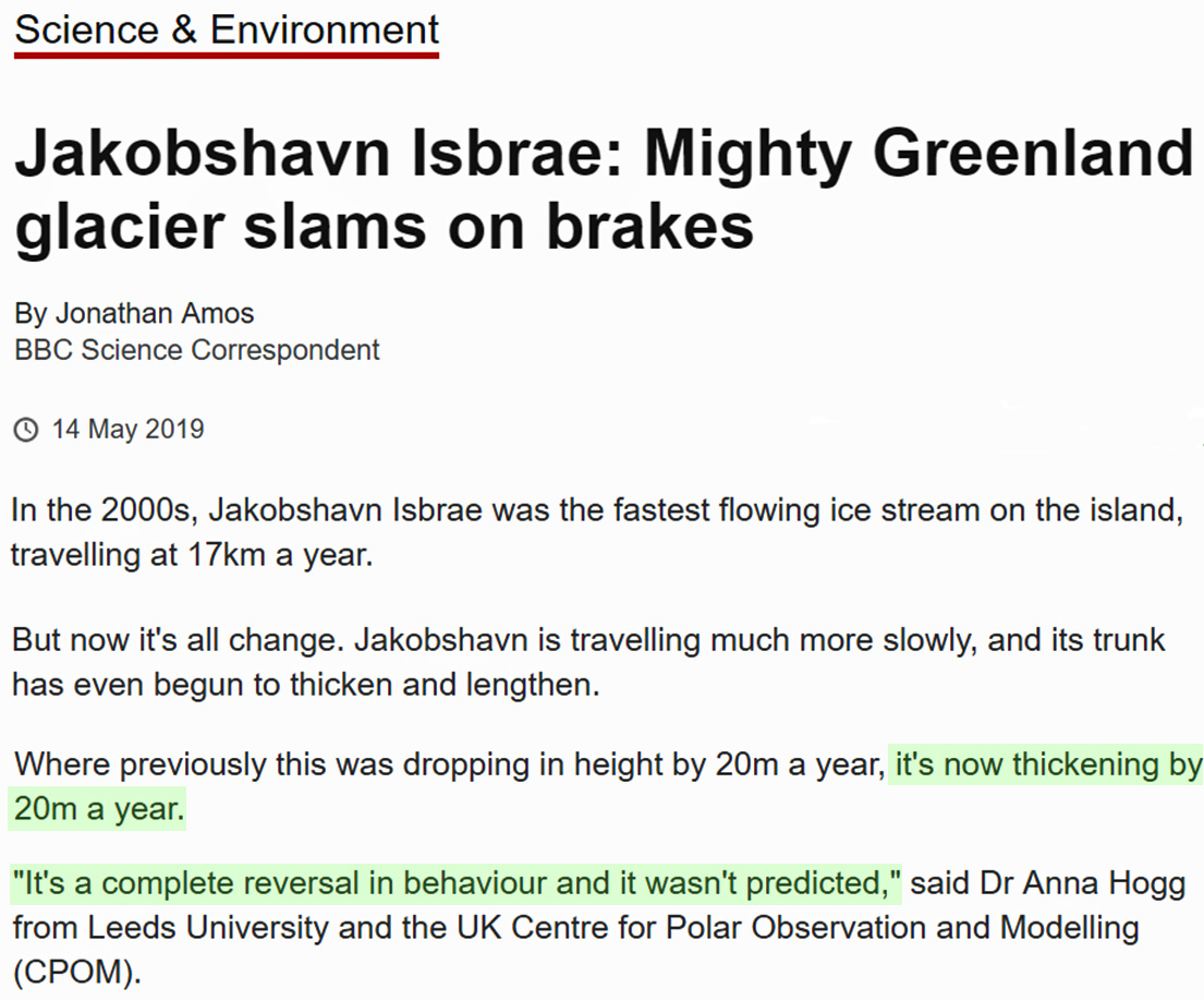
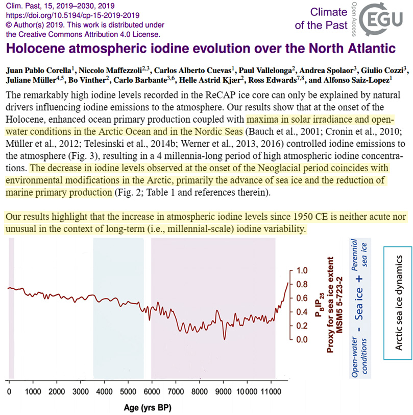
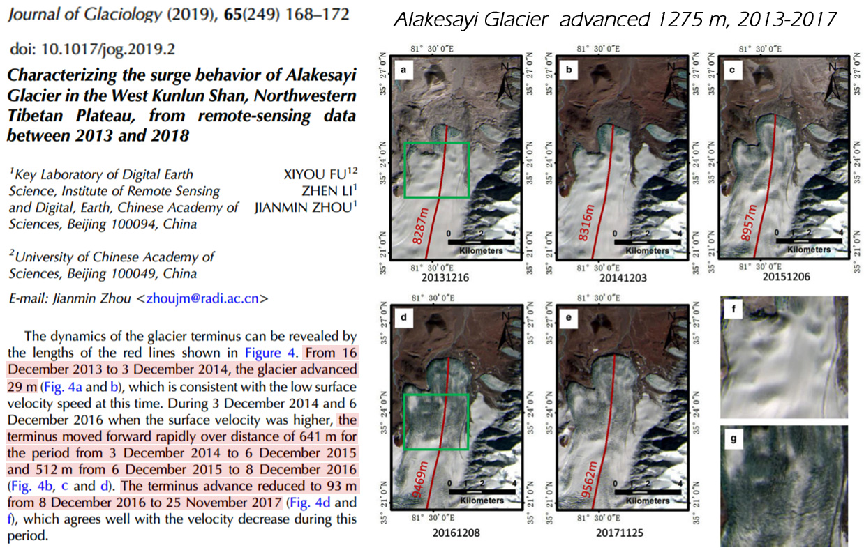
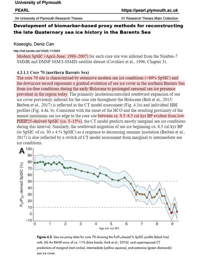
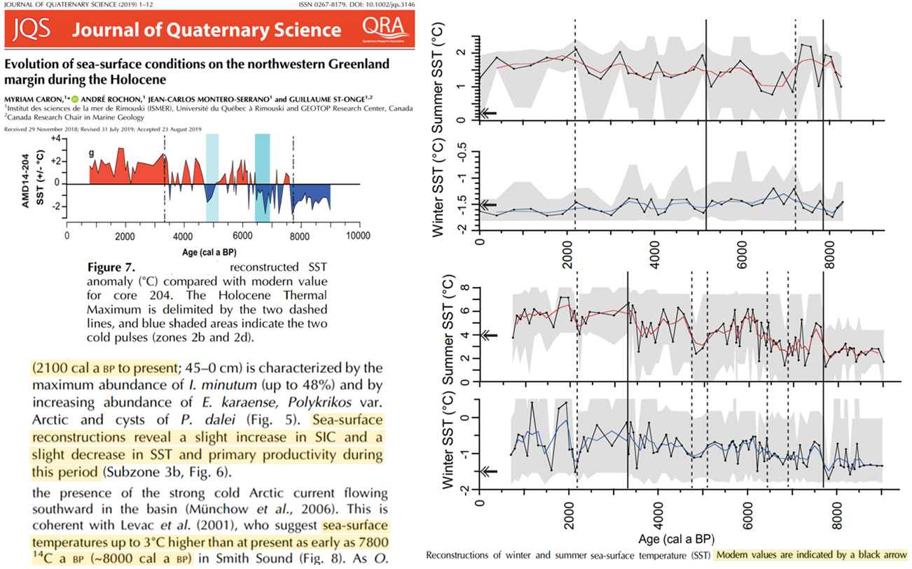
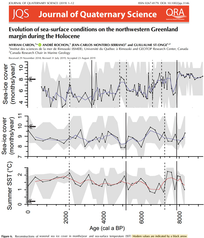
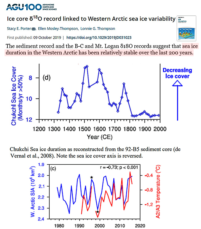
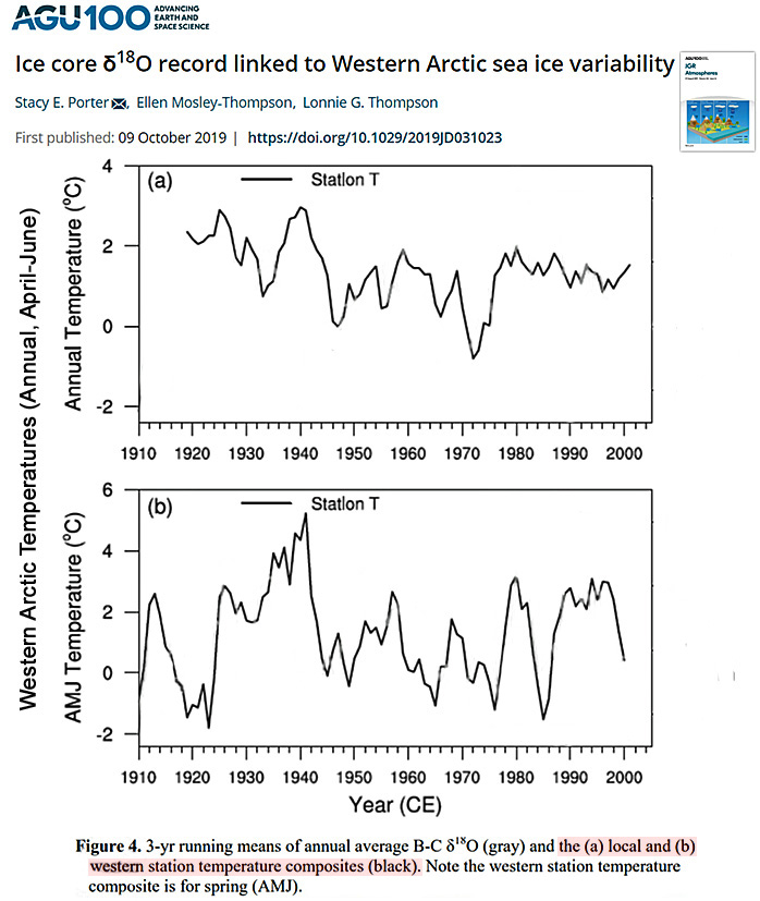
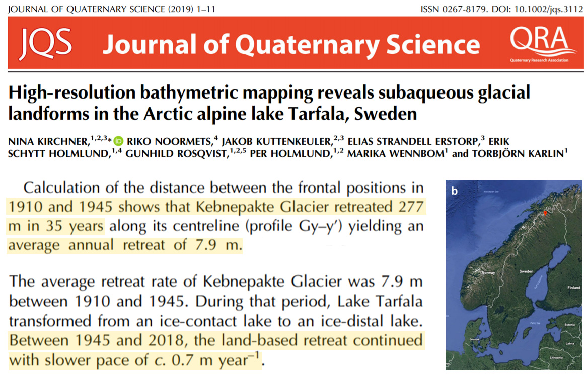
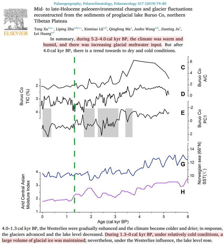
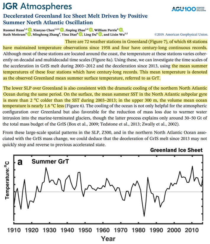
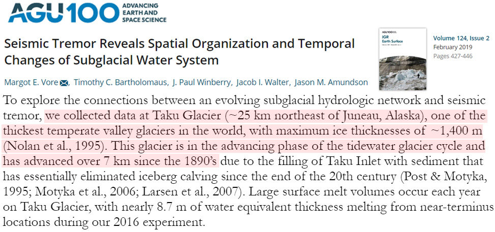
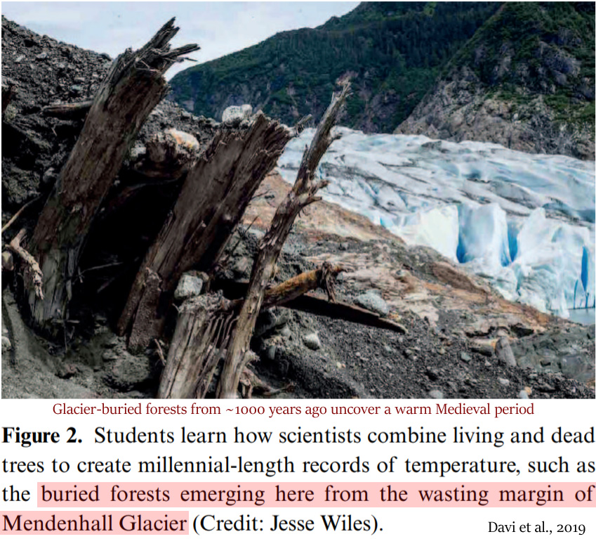
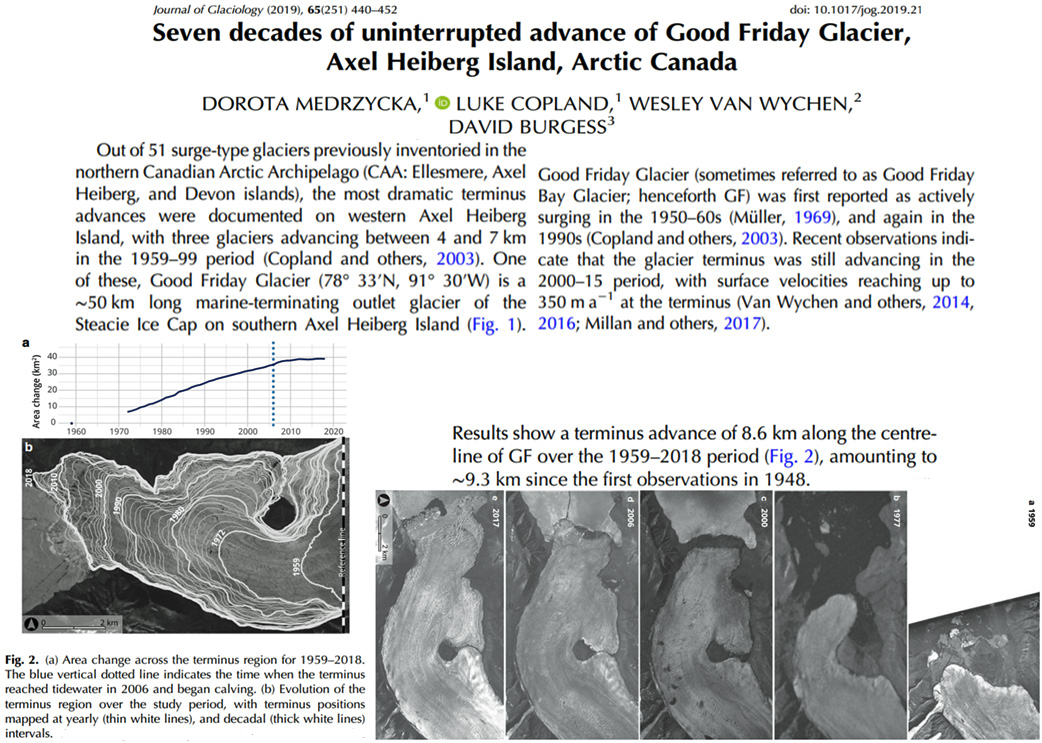
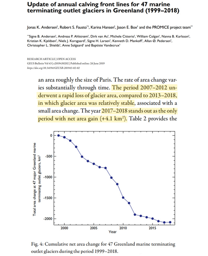
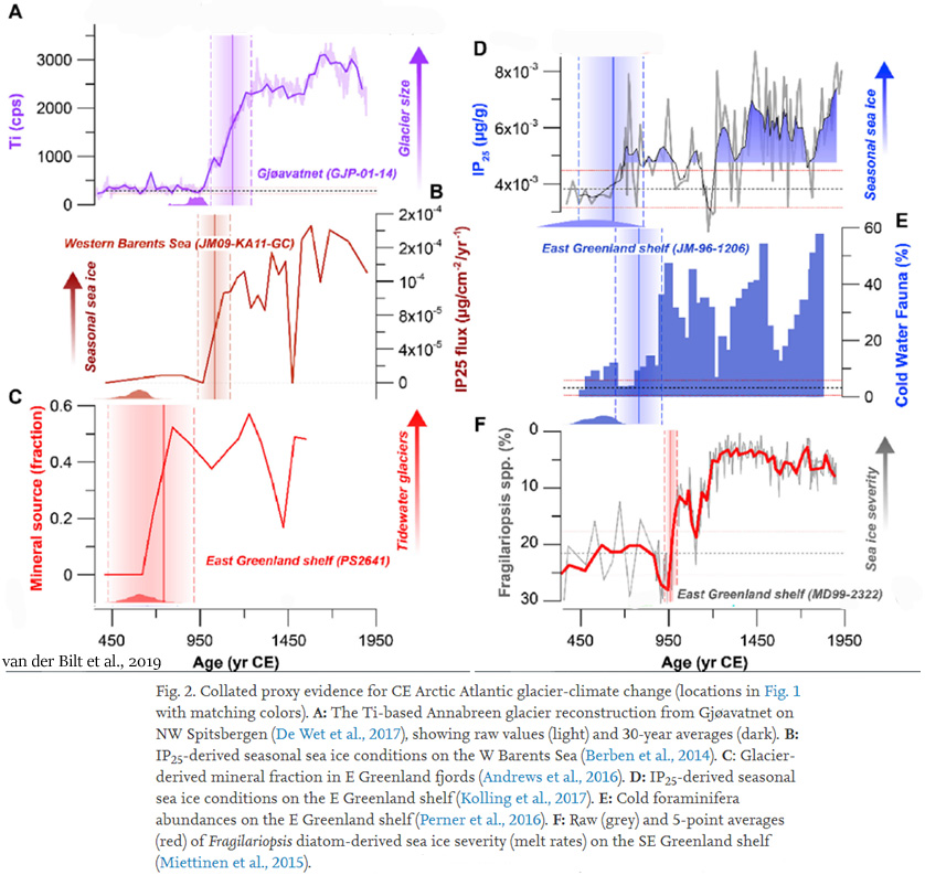
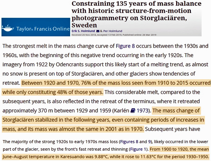
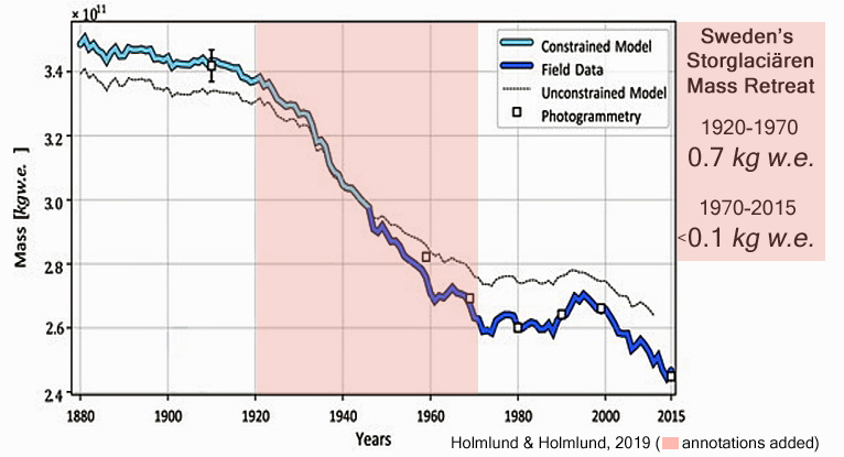
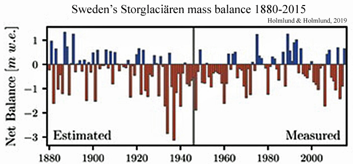
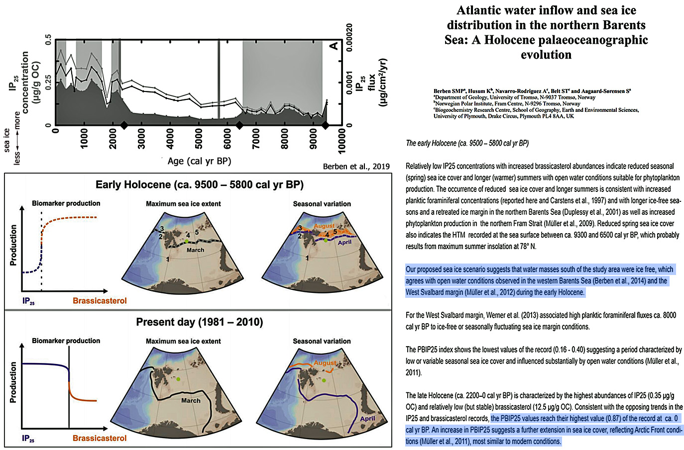
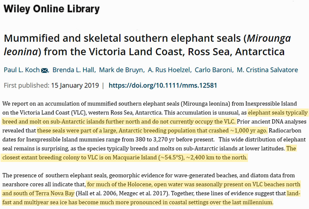
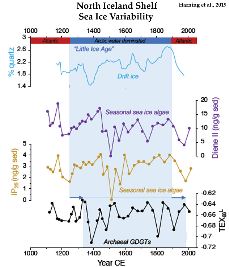
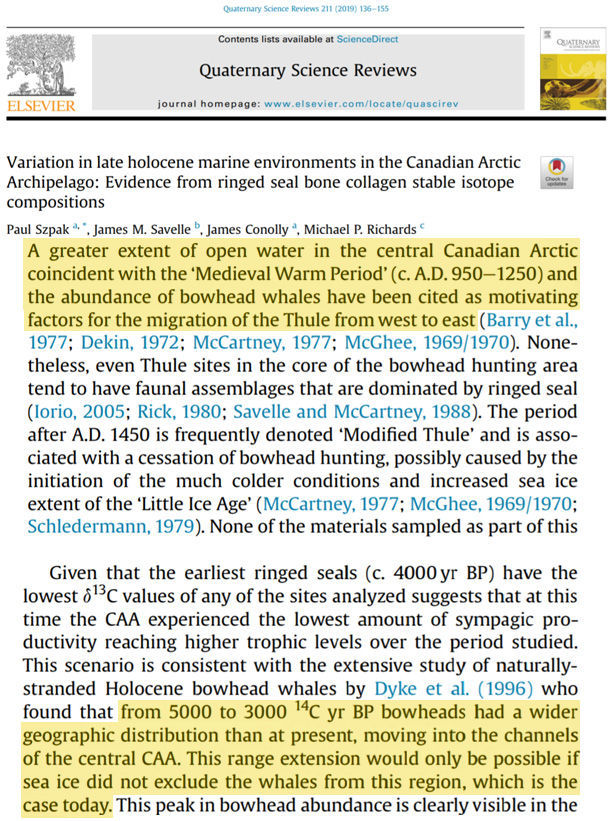
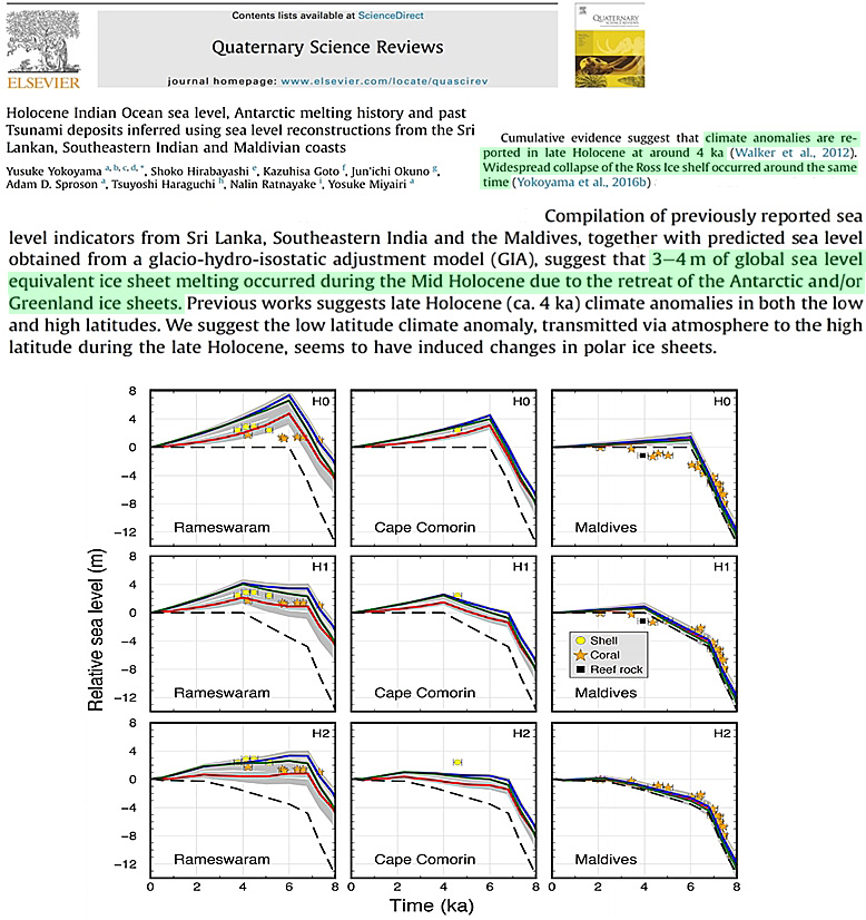
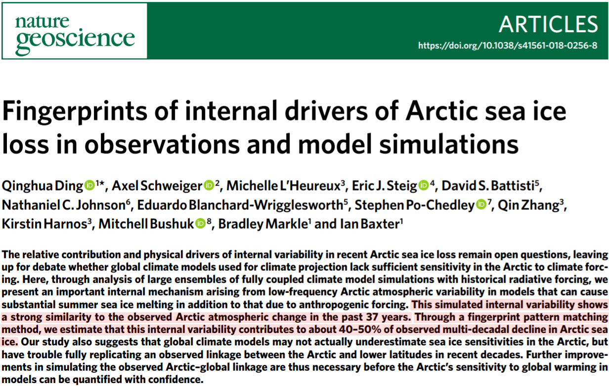
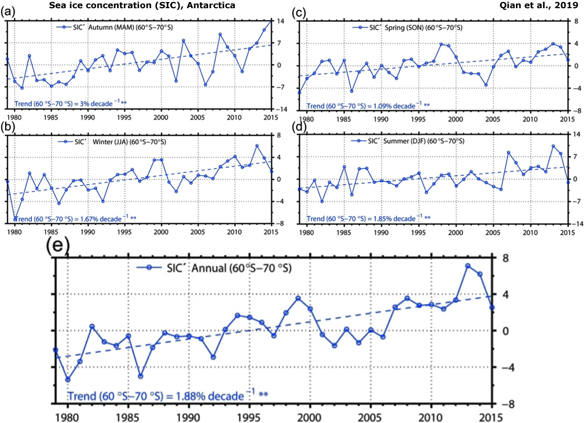
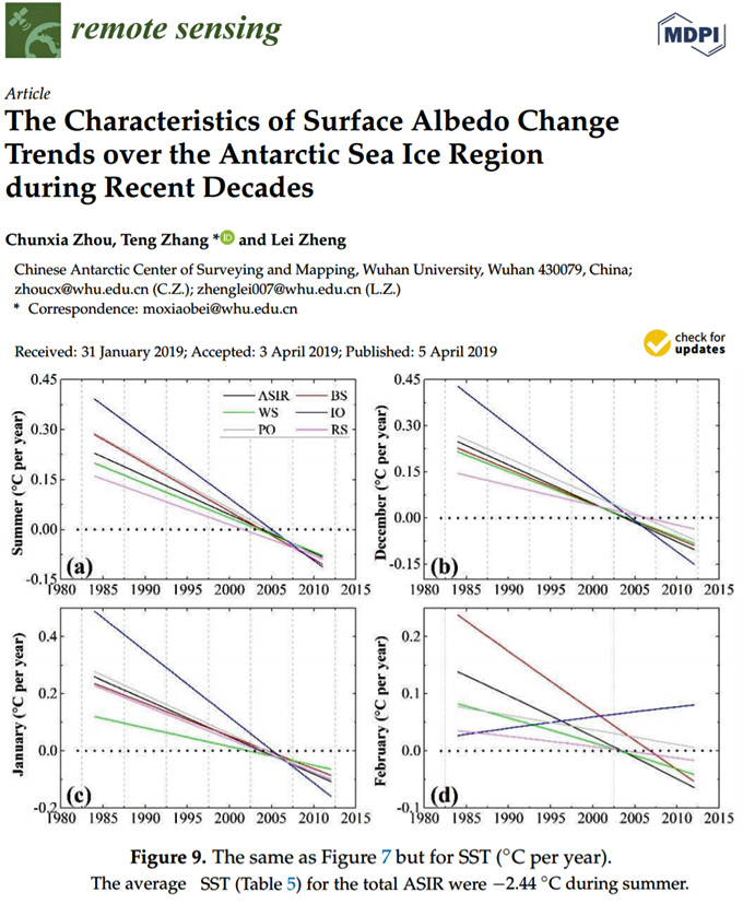
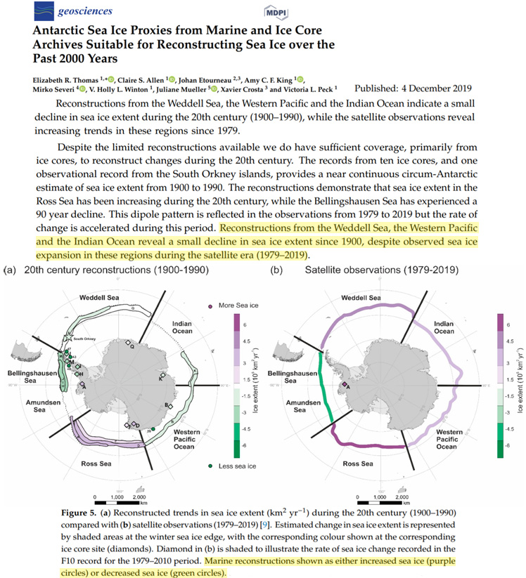
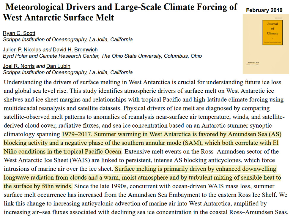
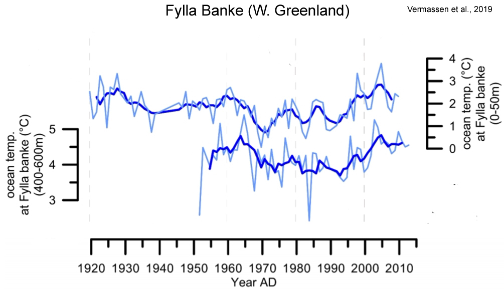
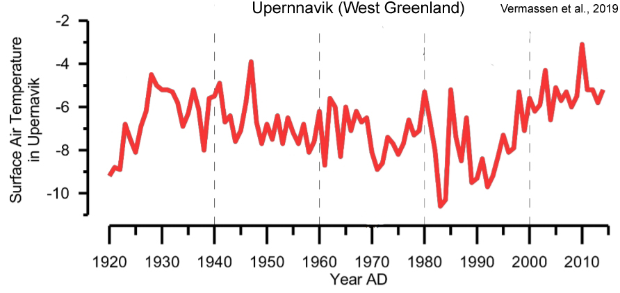
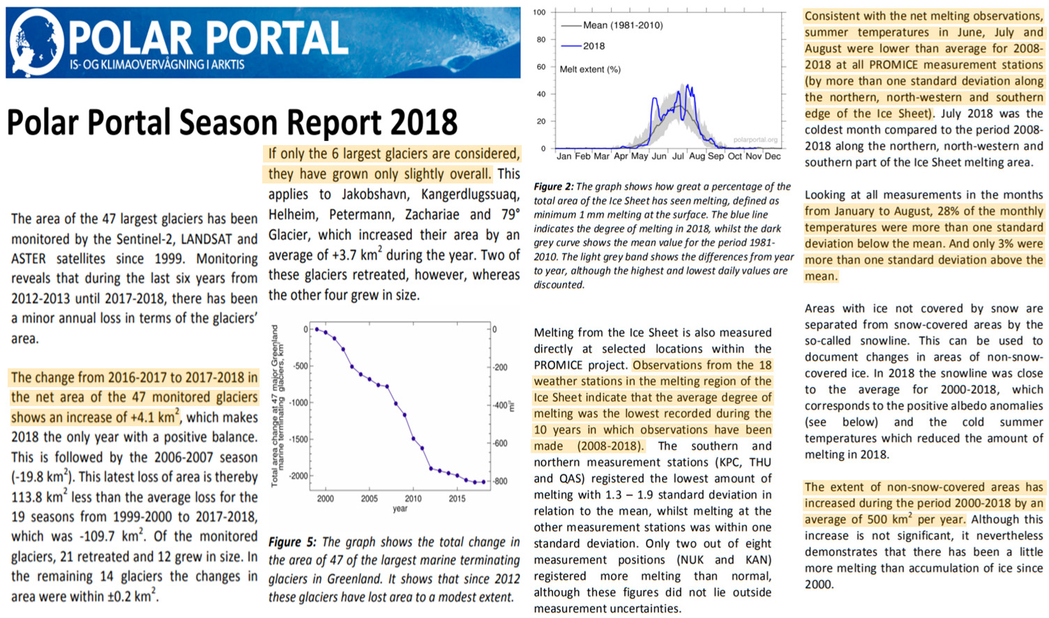
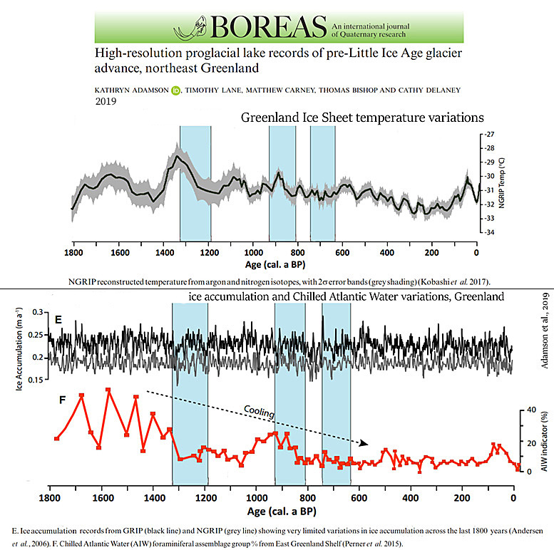
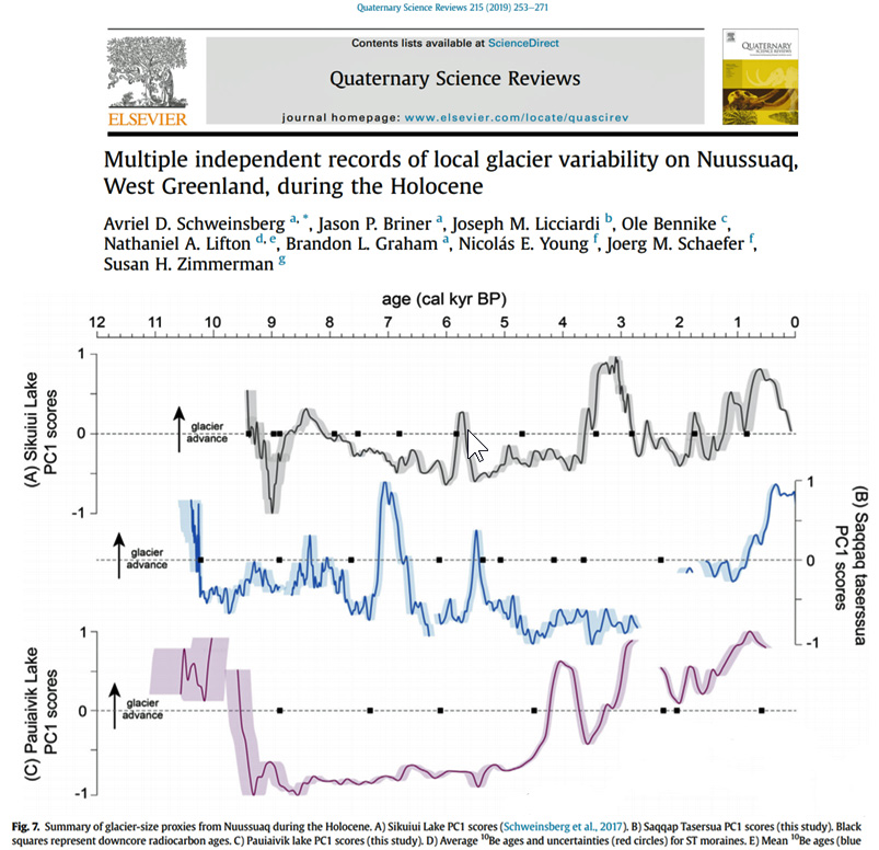
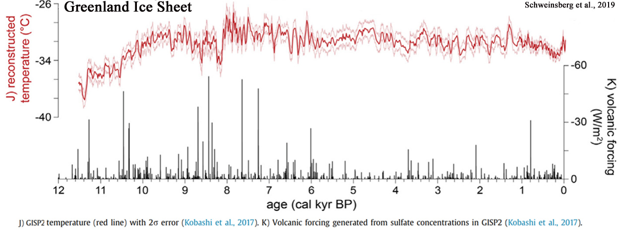
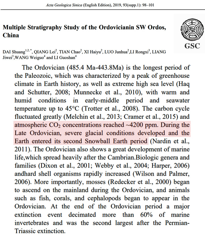
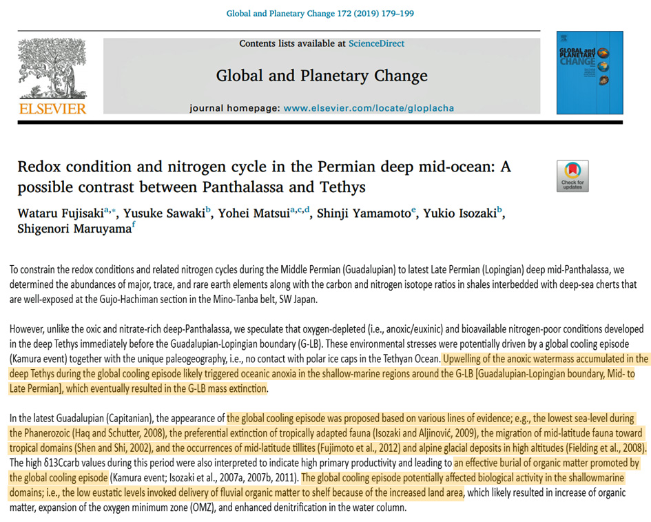
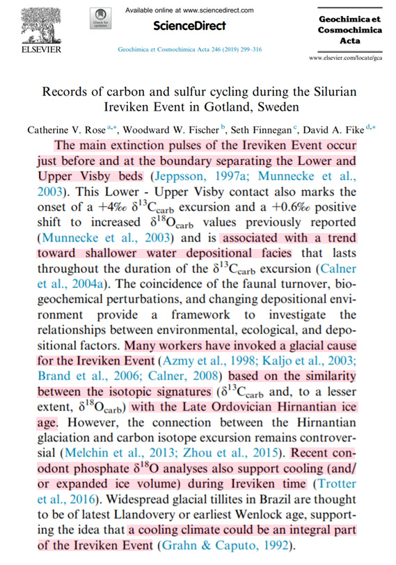
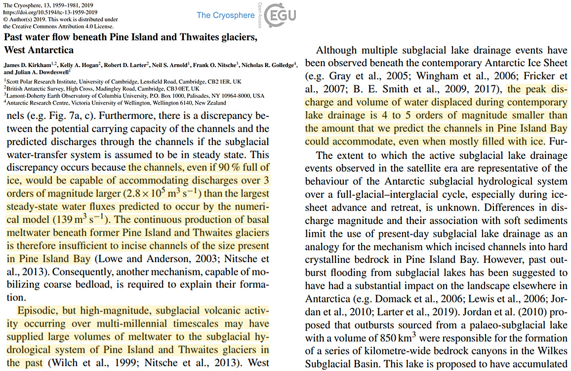
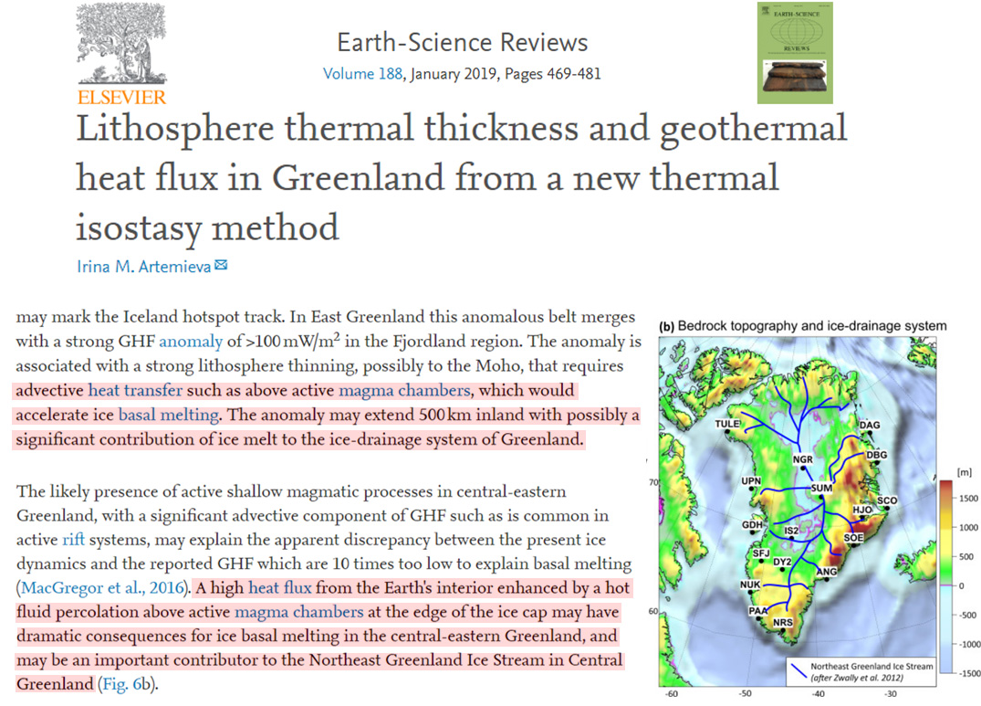
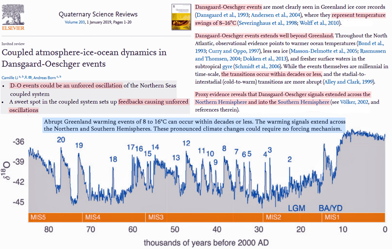
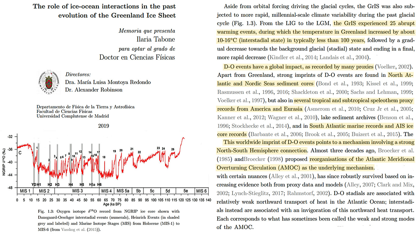


Recent Comments