Solar Influence On Climate
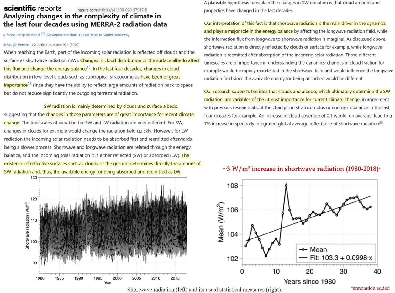
Our research supports the idea that clouds and albedo, which ultimately determine the SW radiation, are variables of the utmost importance for current climate change, in agreement with previous research about the changes in stratocumulus or energy imbalance in the last four decades for example. An increase in cloud coverage of 0.1 would, on average, lead to a 7% increase in spectrally integrated global average reflectance of shortwave radiation. … When reaching the Earth, part of the incoming solar radiation is reflected off clouds and the surface as shortwave radiation (SW). Changes in cloud distribution or the surface albedo affect this flux and change the energy balance. In the last four decades, changes in cloud distribution in low-level clouds such as subtropical stratocumulus have been of great importance since they have the ability to reflect large amounts of radiation back to space but do not reduce significantly the outgoing terrestrial radiation. … [S]hortwave radiation is the main driver in the dynamics and plays a major role in the energy balance by affecting the longwave radiation field … [C]hanges in cloud fraction for example would be rapidly manifested in the shortwave field and would influence the longwave radiation field since the available energy for being absorbed would be different. … The existence of reflective surfaces such as clouds or the ground determines directly the amount of SW radiation and, thus, the available energy for being absorbed and reemitted as LW. … A plausible hypothesis to explain the changes in SW radiation is that cloud amount and properties have changed in the last decades.
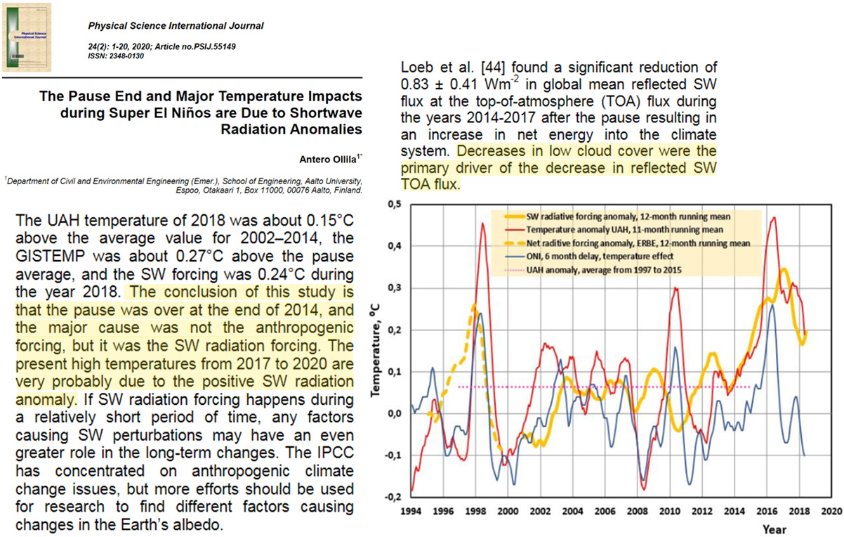
The UAH temperature of 2018 was about 0.15°C above the average value for 2002–2014, the GISTEMP was about 0.27°C above the pause average, and the SW forcing was 0.24°C during the year 2018. The conclusion of this study is that the pause was over at the end of 2014, and the major cause was not the anthropogenic forcing, but it was the SW radiation forcing. The present high temperatures from 2017 to 2020 are very probably due to the positive SW radiation anomaly. If SW radiation forcing happens during a relatively short period of time, any factors causing SW perturbations may have an even greater role in the long-term changes. The IPCC has concentrated on anthropogenic climate change issues, but more efforts should be used for research to find different factors causing changes in the Earth’s albedo. … The positive temperature effect is based on the fact that water vapor as a GH gas is about 12 times stronger than CO2 [59]. … It can be noticed that for 1982–2003, the global temperature anomaly has been increasing but long-term water vapor amount has been decreasing. This observation does not confirm the assumption of most anthropogenic climate models that there is permanent positive water feedback in the atmosphere doubling the warming effects of GH gases.
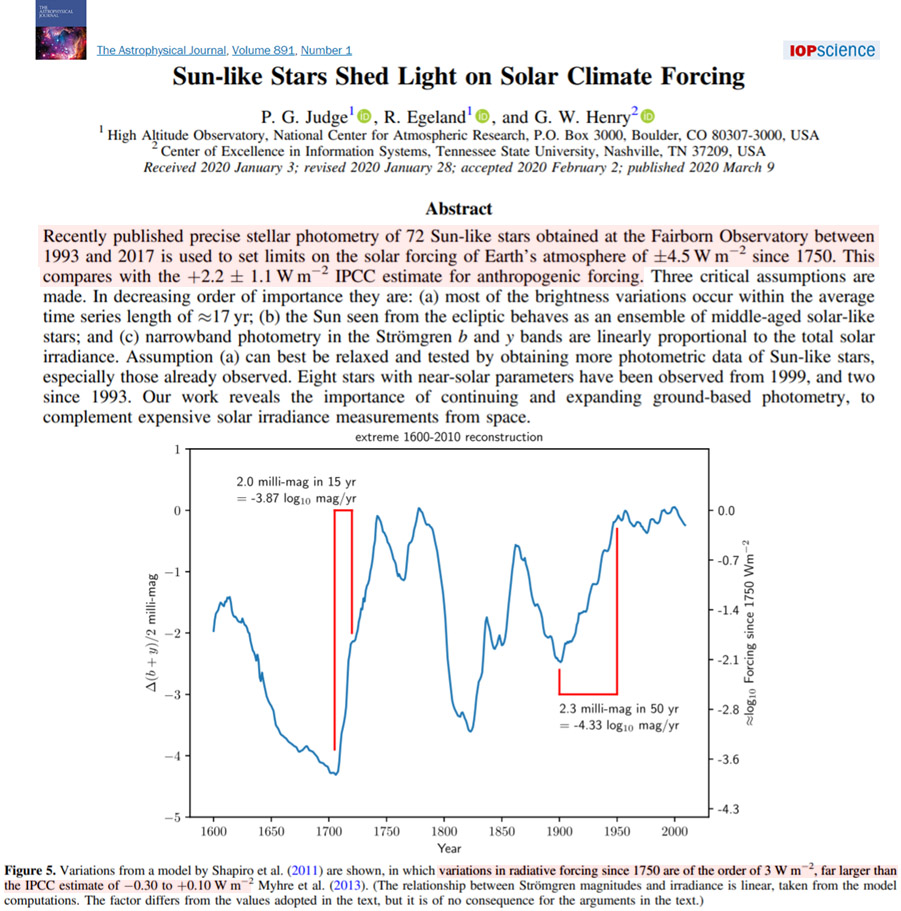
Recently published precise stellar photometry of 72 Sun-like stars obtained at the Fairborn Observatory between 1993 and 2017 is used to set limits on the solar forcing of Earth’s atmosphere of ±4.5 W m−2 since 1750. This compares with the +2.2 ± 1.1 W m−2 IPCC estimate for anthropogenic forcing. … [V]ariations in [solar] radiative forcing since 1750 are of the order of 3 W m−2, far larger than the IPCC estimate of −0.30 to +0.10 W m−2 Myhre et al. (2013).
The cool and humid climate during the early Holocene limited the spread of fire, while warming and drying at ~7.6 cal ka BP triggered higher fire occurrence. Instead of temperature, changes in precipitation dominated fire regime variation during the mid- to late Holocene. On millennial timescales, we suggest that Holocene fire variability has been predominantly controlled by the combined effects of Northern Hemisphere (NH) summer and winter insolation that influenced monsoonal precipitation and fire season temperature, respectively.
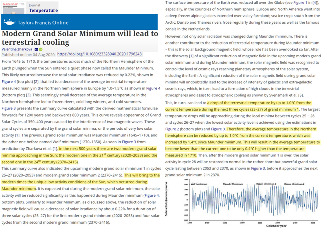
A significant reduction of the solar magnetic field during grand solar minima will undoubtedly lead to the increase of intensity of galactic and extra-galactic cosmic rays, which, in turn, lead to a formation of high clouds in the terrestrial atmospheres and assist to atmospheric cooling as shown by Svensmark et al. [5]. … [T]he reduction of solar magnetic field will cause a decrease of solar irradiance by about 0.22% for a duration of three solar cycles (25–27) for the first modern grand minimum (2020–2053) and four solar cycles from the second modern grand minimum (2370–2415). This, in turn, can lead to a drop of the terrestrial temperature by up to 1.0°C from the current temperature during the next three cycles (25–27) of grand minimum 1. The largest temperature drops will be approaching during the local minima between cycles 25 − 26 and cycles 26–27 when the lowest solar activity level is achieved using the estimations in Figure 2 (bottom plot) and Figure 3. Therefore, the average temperature in the Northern hemisphere can be reduced by up to 1.0°C from the current temperature, which was increased by 1.4°C since Maunder minimum. This will result in the average temperature to become lower than the current one to be only 0.4°C higher than the temperature measured in 1710.
Sharabian and Karakouzian, 2020
Results indicated that a distinct 8–12-year correlation exists between the two time series of SSN [sunspot number] and MAP [mean annual precipitation], and peaks in precipitation mostly occur one to three years after the SSN maxima.
Even energetically small factors may have a big influence on climate change. In our opinion, the most important of these factors are cosmic rays and cosmic dust through their influence on clouds, and thus, on climate. … Due to the increasing of Solar Wind with a increment of Cosmic rays and the increment of sunspot has a wide impact on the Space Weather, causes Global Warming.
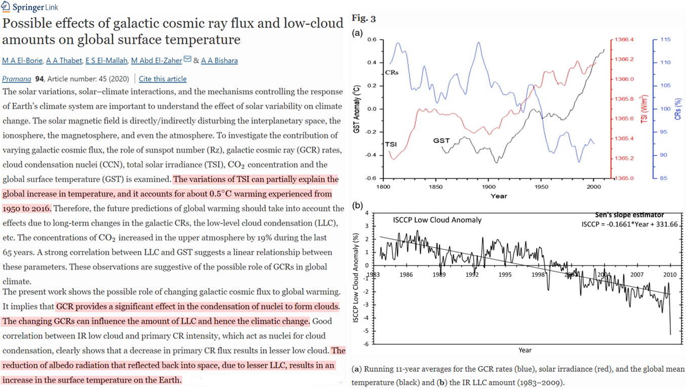
The variations of TSI can partially explain the global increase in temperature, and it accounts for about 0.5∘C warming experienced from 1950 to 2016. Therefore, the future predictions of global warming should take into account the effects due to long-term changes in the galactic CRs, the low-level cloud condensation (LLC), etc. The concentrations of CO2 increased in the upper atmosphere by 19% during the last 65 years. A strong correlation between LLC and GST suggests a linear relationship between these parameters. These observations are suggestive of the possible role of GCRs in global climate. … [T]he TSI shows an increase of 0.75W/m2 during the epoch 1800–2008. These results show that there is a 56% increase of solar activity, as well as the magnetic field, which reduces the GCR from reaching the atmosphere by 19% and as a result the GST increases.
Many studies have investigated the role of solar variability in Holocene climate. Beyond sun spot observations, solar activity can be reconstructed from 14C in tree rings. Due to the lack of sub-decadal resolution of 14C records, these studies focused on long-term processes. In this study, we use an annually-resolved 14C record to examine solar variability (e.g. 11-year Schwabe solar cycle) and its connection to European seasonal climate inferred from tree-ring records during the entire past millennium with spectral and wavelet techniques. The 11-year Schwabe solar cycle shows a significant impact in European moisture- and temperature-sensitive tree-ring records. Complex ‘top-down’ / ‘bottom-up’ effects in the strato-tropoatmospheric system are assumed to affect European spring and summer climate with a temporal-shift as evident from observed changes in phase behavior. Significant evidence is also found for the ~60- and ~90-year band during the first half of the past millennium.
Spectral analysis reveals that bulliform abundance and reconstructed climate vary with a major ~1000-year periodicity during the Holocene, suggesting a possible causal relationship to solar activity. A high bulliform abundance and warm-dry climate correspond with enhanced solar activity, and vice versa.
Moisture fluctuations showed three distinct stages (extremely dry between 742BC and ~AD500, relatively wet with an increasing trend between ~AD500 and 1200 and relatively wet with frequent fluctuations after AD1200), interrupted by 14 drought events. Spectral analysis and continuous wavelet transform of moisture variation revealed 200- and 120-year cycles. According to cross-wavelet transform analysis, major drought frequency of ~200-year was explicitly correlated to solar activity. It’s suggested that the centennial-scale drought frequency was mainly driven by solar activity, through modulation of large-scale atmospheric circulation.
In particular, we observe that the four main intervals of lower and higher temperatures correspond to periods of low and high solar activity, respectively. Furthermore, our SST patterns are similar in phase and amplitude to the general patterns of the solar activity. Solar activity variations are a global rather than a regional phenomenon hence solar activity also correlates with the ice dynamics of the important glaciated regions of the globe. For example, at ∼2.8 to 3.7 ka (interval II) and at ∼4.4 to 4.9 ka (interval IV) low temperature patterns correspond to times of glacial advances in several parts of the world, including the Alps, Scandinavia, Himalayas, Alaska, New Zealand and Patagonia (Grove, 2004; Thompson et al., 2006). At regional scale, this interpretation is also in agreement with the SST records from the Eastern Pacific where colder temperatures between ∼2.8 and 3.8 ka and ∼4.1 and 4.9 ka were reported (Koutavas et al., 2002). Furthermore, our findings are in accord with high SSTs reported at ∼4 and 1.8 ka to 2.9 ka (Koutavas et al., 2002; Abram et al., 2009) in the Southern Pacific. This indicates that, first, the reported SST variability on the order of up to ± 2◦C reflects the global temperature oscillations throughout the Mid to Late Holocene, and second, that solar activity seems to be the major driver of centennial to millennial scale SST changes throughout the Mid to Late Holocene, at least in the Southern Pacific.
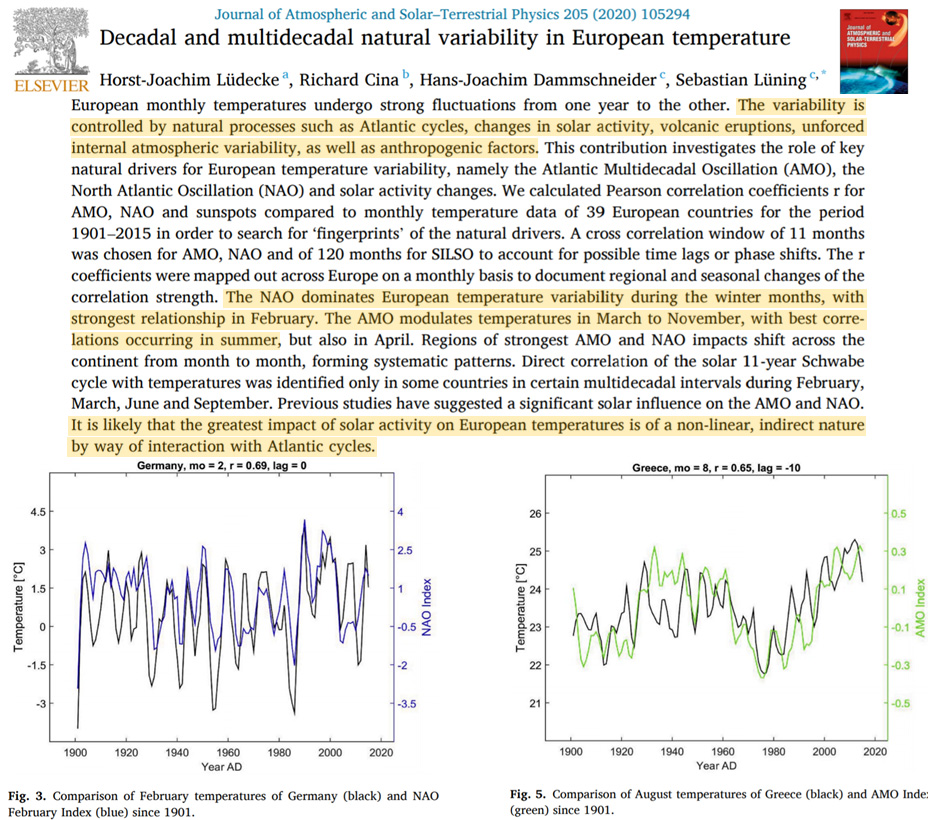
The NAO dominates European temperature variability during the winter months, with strongest relationship in February. The AMO modulates temperatures in March to November, with best correlations occurring in summer, but also in April. Regions of strongest AMO and NAO impacts shift across the continent from month to month, forming systematic patterns. Direct correlation of the solar 11-year Schwabe cycle with temperatures was identified only in some countries in certain multidecadal intervals during February, March, June and September. Previous studies have suggested a significant solar influence on the AMO and NAO. It is likely that the greatest impact of solar activity on European temperatures is of a non-linear, indirect nature by way of interaction with Atlantic cycles.
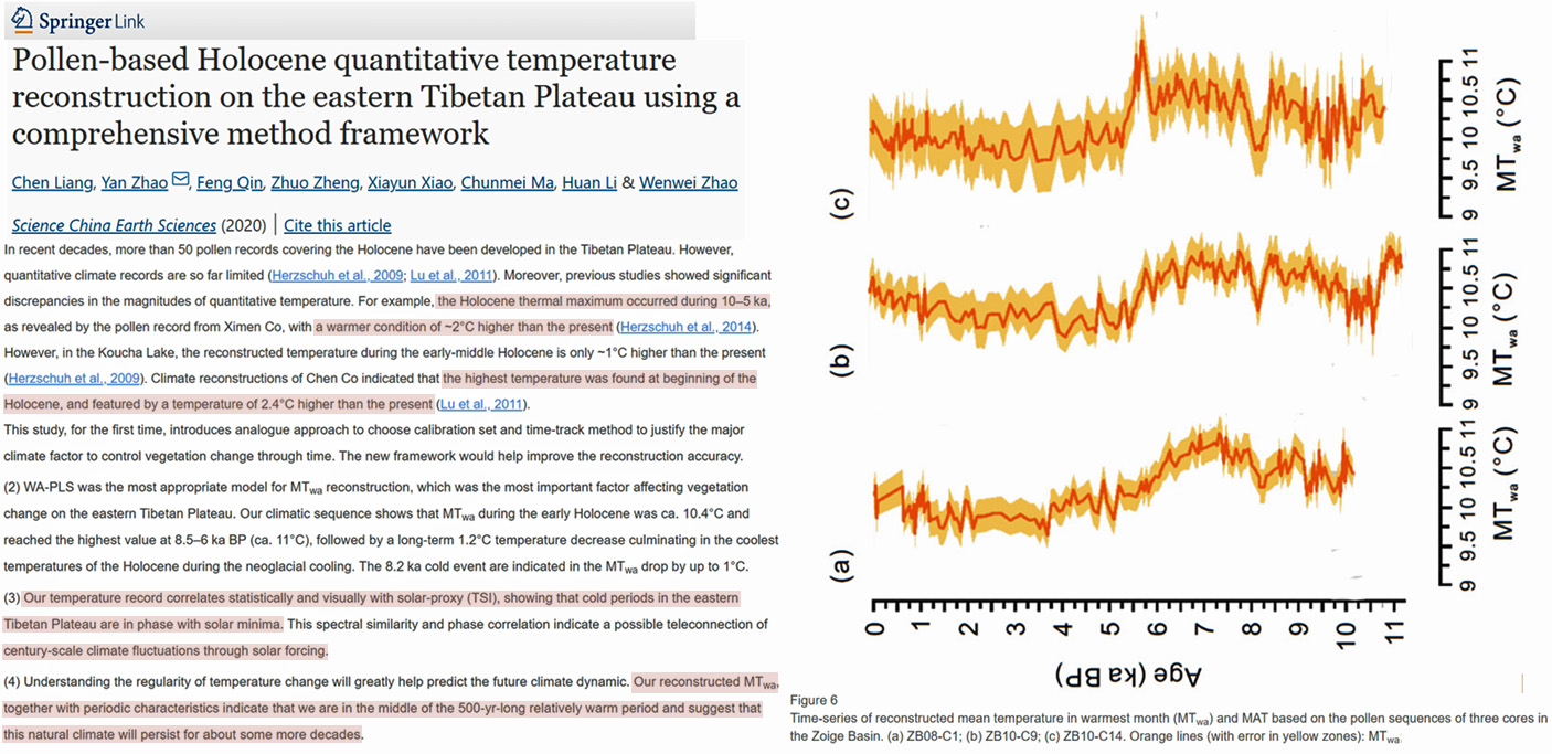
Our climatic sequence shows that MTwa [warmest month] during the early Holocene was ca. 10.4°C and reached the highest value at 8.5–6 ka BP (ca. 11°C), followed by a long-term 1.2°C temperature decrease culminating in the coolest temperatures of the Holocene during the neoglacial cooling. The 8.2 ka cold event are indicated in the MTwa drop by up to 1°C. … [T]he Holocene thermal maximum occurred during 10–5 ka, as revealed by the pollen record from Ximen Co, with a warmer condition of ~2°C higher than the present (Herzschuh et al., 2014). However, in the Koucha Lake, the reconstructed temperature during the early-middle Holocene is only ~1°C higher than the present (Herzschuh et al., 2009). Climate reconstructions of Chen Co indicated that the highest temperature was found at beginning of the Holocene, and featured by a temperature of 2.4°C higher than the present (Lu et al., 2011). … Our temperature record correlates statistically and visually with solar-proxy (TSI), showing that cold periods in the eastern Tibetan Plateau are in phase with solar minima. This spectral similarity and phase correlation indicate a possible teleconnection of century-scale climate fluctuations through solar forcing. … Understanding the regularity of temperature change will greatly help predict the future climate dynamic. Our reconstructed MTwa, together with periodic characteristics indicate that we are in the middle of the 500-yr-long relatively warm period and suggest that this natural climate will persist for about some more decades.
Spectrum analysis of the water-table profile yielded a statistically significant periodicity of 470-year that may be related to the “~500-year” inherent solar irradiation cycles. In addition, positive correlation between the peatland water-table levels and cosmic-isotope-reconstructed sunspot numbers underscores the role of the sun in regulating hydrological processes in the EASM margin area. The data suggest that the regional climate and hydrological variations at the EASM margin were first triggered by changes in solar output, but may have been amplified by interactions with oceanic and atmospheric circulations.
Influence of the sun on climate becomes underestimated when the 22-year Hale12 cycle is ignored in climate science … With this correction, the combination of the primary and secondary minima shows for the period 1890-1985 a high solar sensitivity: 1,143°C per W/m2. This also implies that the Sun caused a warming of 1,07°C between Maunder minimum and solar minimum year 2017, well over half of the intermediate temperature rise of approximately 1,5°C. The 22-year cycle forms a crucial factor for better understanding the Sun-temperature relation. Ignoring the 22- year cycle leads to underestimation of the Sun’s influence in climate change (+ overestimation of anthropogenic factors and greenhouse gases such as CO2).
There are no fool proof evidences that the solar variations are a major factor in driving recent global climate change but there are considerable evidences of solar influence on the climate of particular regions as well as throughout the terrestrial environment. During high solar activity, higher temperatures and larger ozone concentrations are observed in the tropical stratosphere. The solar influences on the Earth’s climate mainly includes; the changed occurred due to variations in the Sun’s radiant output (TSI and UV) and the changes occurred due to the Sun’s influence on the energetic particles reaching to the Earth (Solar Energetic Particles, Galactic Cosmic Rays). Following the above regime, we have provided the evidences for the existence of physical links between solar activity and terrestrial climate.
Eight proxy records of Northern Fennoscandian summer temperature variability were analyzed for the CE 1700–2000 period. Stable and statistically significant correlation between the summer temperature reconstructions and a quasi 22-year Hale solar cycle was found to be present through the entire study period. The revealed solar–climatic link is a result of the effect of a weak solar cycle signal on a climatic system having internal bi-decadal variability. Precise physical mechanisms to explain this link are far from clear but galactic cosmic ray flux appears a probable physical agent to mediate the solar effect to the lower troposphere.
The 50- and 2.0–3.0-year cycles of this reconstruction were consistent with other tree-ring based hydrometeorological reconstructions, and revealed the possible influences of the Gleissberg solar activity cycle and the interannual oscillations of land atmospheric–ocean systems.
Solar activity has alternated between active and quiet phases with a period of approximately 11 years for each phase (Nagovitsyn 1997). The 11-year cycle in the reconstructed PDSI series, which was detected by cycle analyses, suggests a strong possible connection with the Schwabe cycle of solar activity. The 22-year cycle in the reconstruction corresponded to the 22-year Hale cycle, i.e. the double harmonic of the 11-year cycle. Interannual (2.3- and 2.1-year) cycles in this reconstruction might fall within the Quasi-Biennial Oscillation (Baldwin et al. 2001). These interdecadal and interannual cycles in the PDSI reconstruction might be influenced both by solar activity and by the oscillations of land–atmosphere–ocean circulation systems.
[A] number of scientists has reported some kind of relationship between solar activity and earthquake occurrence; or among global seismicity and geomagnetic variation or magnetic storms. … In this paper, we will definitively establish the existence of a correlation between solar activity and global seismicity, using a long data set and rigorous statistical analysis. … We found clear correlation between proton density and the occurrence of large earthquakes…with a probability to be wrong lower than [1/100,000]. … [W]e demonstrate that it can likely be due to the effect of solar wind, modulating the proton density and hence the electrical potential between the ionosphere and the Earth.
The average water level in the Puck Lagoon rose by ca. 0.85 m during the last 1500 years in a cyclic mode, with a period cycle of ca. 600–550 years and an amplitude not exceeding 0.5 m. The accelerated sea level rise and frequent storminess occurred during the first half of the Dark Ages (1500−1300 years b2k) and LIA (750−450 years b2k) and since the beginning of the 20th century. Recognized environmental changes are well correlated with both temperature changes in the North Atlantic and changes in total solar irradiance, suggesting synchronous Northern Hemisphere-wide fluctuations. The solar forcing was an important constituent of natural climate variability in the past and of forcing climate warming during modern times – after the Little Ice Age. Thus, the accelerated sea level rise during the first half of the Dark Ages and LIA could be 1.5–1.7 mm/year, that is, similar to that observed over the last century (Figure 11).
The centennial-scale cold events were synchronous with stages of low solar activity. Spectral and cross-spectral analyses demonstrate that summer temperature and solar activity have a common cyclicity, and we therefore suggest that solar activity was the fundamental driver of the centennial-scale variability of summer temperature in ACA during the Holocene.
The present work examines and discusses the response of the atmospheric layers to solar variations, whereas the solar outputs are responsible for the changes in the Earth’s environment. Galactic cosmic ray rates (GCRs), solar cycle lengths (SCLs), sunspots (Rz), coronal index (CI) of solar activities, the aa geomagnetic activity index, total solar irradiance (TSI), CO2 concentrations, global surface temperatures (GSTs), the near-Earth of the northern and southern hemispheres temperatures have been examined. Our results displayed that every SCL has different behaviors to the sensitivity of GST, according to different modulations of GCRs by solar wind/helio-magnetic field parameters. Lower cosmic rays and higher solar irradiance and geomagnetic activity occur when solar activity increases. Furthermore, the average sensitivities of global temperature to geomagnetics aa and total solar irradiance and in turn low-level cloud cover are significant and real. Our results could indicate that geomagnetic disturbances, which driven by the solar wind, may influence global temperature. Both correlations of GST–Rz displayed the same behavior to the end of SC 22nd, and a great discrepancy is observed during the SC 23rd. The observed correlations of Rz with NH and SH temperatures displayed different behaviors. Four different mechanisms are involved in the direct/indirect effect of TSI variations on the Earth’s atmosphere and temperatures.
These magnetic and grain size records indicate that EASM intensity followed a general declining trend between approximately 6800 and 2000 cal yr BP. This general pattern is synchronous with other geologic archives from monsoon regions, and can be attributed to solar radiation forcing in the Northern Hemisphere. On centennial timescales, a weak EASM closely coincides with periods of weak solar activity. In addition, spectral analysis of clays reveals five prominent cycles, with periodicities of approximately 364, 202, 158, 119, and 104 years, which correspond to solar activity cycles. The similarities between the cyclicities of the Asian monsoon signal in sedimentary records and those of solar activity demonstrate that solar forcing has a relatively large influence on the centennial-scale variability of the EASM.
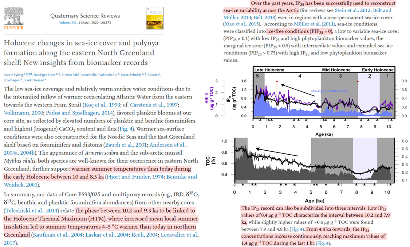
Warmer sea-surface conditions were also reconstructed for the Nordic Seas and the East Greenland shelf based on foraminifers and diatoms (Bauch et al., 2001; Andersen et al., 2004a, 2004b). The appearance of Armeria scabra and the sub-arctic mussel Mytilus edulis, both species are well-known for their occurrence in eastern North Greenland, further support warmer summer temperatures than today during the early Holocene between 10 and 8.5 ka (Hjort and Funder, 1974; Bennike and Weidick, 2001). … In summary, our data of Core PS93/025 and multiproxy records (e.g., IRD, δ18O, δ13C, benthic and planktic foraminifera abundances) from other nearby cores (Telesiński et al., 2014) relate the phase between 10.2 and 9.3 ka to be linked to the Holocene Thermal Maximum (HTM), where increased mean local summer insolation led to summer temperatures 4–5 °C warmer than today in northern Greenland (Kaufman et al., 2004; Laskar et al., 2004; Reeh, 2004; Lecavalier et al., 2017). … Spectral analysis reveals significant power at frequencies exceeding the 90% confidence level and corresponding to periodicities of 110–130, 170, 220 and 500 years in the proxy records of IP25, HBI III and brassicasterol throughout the Holocene (Fig. 9). Such short-term cycles of 110–130 year periods have been observed in the oxygen isotope record of the NGRIP (NGRIP-Members, 2004) and are likely linked to variations in solar activity (Vonmoos et al., 2006). A spectral power centered around a period of 200 years (brassicasterol) may correspond to the De Vries/Suess cycle of solar activity. North Atlantic variability at this timescale has been previously found in the 512 year Δ14C cycle and is connected to variabilities in the North Atlantic Deep Water Formation (NADW) (Stuiver and Braziunas, 1993). While the exact period of spectral peaks may be biased by uncertainties in the age model, the correspondence between our and other oceanic and terrestrial variations in paleoclimate proxies with cyclic signals in solar activity (Stuiver et al., 1995; Ito and Yu, 1999; Chapman and Shackleton, 2000; Hu et al., 2003; Zhao et al., 2010) suggests a possible key role of the amount of total solar irradiance as a driver of oceanic and atmospheric change in the Arctic region.
[A]t this site, the LIA was not recorded as a continuously cold period, but involved two cold phases that correlated with the Spörer (AD 1450–1550) and Maunder (AD 1650–1750) minima in solar activity (Lozano-García et al., 2007). The diatom, ostracod, and geochemical record from Lake Santa María del Oro in western Mexico (Figure 1) showed that the LIA (AD 1450) was a period of low lake level and dry conditions (Rodríguez-Ramírez et al., 2015), which was also inferred from the δ18O from gastropod record from Aguada X’camaal, in the Yucatán Peninsula (Hodell et al., 2005). Previous research at Lake La Luna in central Mexico also reported dry conditions (based on low magnetic susceptibility values) during the LIA; however, at this site, the driest interval correlated with the Maunder solar minimum (Cuna et al., 2014).
The δ18O record, if viewed as a proxy of the Asian summer monsoon (ASM) intensity, provides an ASM history for the early Holocene with clear centennial-scale variability. A significant approximately 200-yr cycle between 10.2 and 9.1 ka BP (before present, where “present” is defined as the year AD 1950), as revealed by spectral power analyses, is of global significance and is probably forced by the Suess or de Vries cycle of solar activity. We argue that the centennial fluctuations of the ASM [Asian Summer Monsoon] are a fundamental characteristic forced by the solar activity, with the ENSO variability as a mediator. The relationship between ENSO and the ASM displayed spatial heterogeneity on the centennial scale during the early Holocene, which is a more direct analogue to the observed modern interannual variability of the ASM.
Many studies have investigated the role of solar variability in Holocene climate. Beyond sun spot observations, solar activity can be reconstructed from 14C in tree rings. Due to the lack of sub-decadal resolution of 14C records, these studies focused on long-term processes. In this study, we use an annually-resolved 14C record to examine solar variability (e.g. 11-year Schwabe solar cycle) and its connection to European seasonal climate inferred from tree-ring records during the entire past millennium with spectral and wavelet techniques. The 11-year Schwabe solar cycle shows a significant impact in European moisture- and temperature-sensitive tree-ring records. Complex ‘top-down’ / ‘bottom-up’ effects in the strato-tropoatmospheric system are assumed to affect European spring and summer climate with a temporal-shift as evident from observed changes in phase behavior. Significant evidence is also found for the ~60- and ~90-year band during the first half of the past millennium.
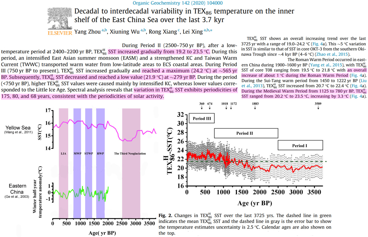
During Period II (2500–750 yr BP), after a lowtemperature period at 2400–2200 yr BP, TEXH86 SST increased gradually from 19.2 to 23.5 °C. During this period, an intensified East Asian summer monsoon (EASM) and a strengthened KC and Taiwan Warm Current (TWWC) transported warm water from low-latitude areas to ECS coastal areas. During Period III (750 yr BP to present), TEXH 86 SST increased gradually and reached a maximum (24.2 °C) at ~565 yr BP. Subsequently, TEXH 86 SST decreased and reached a low value (21.9 °C) at ~279 yr BP. During the period (<750 yr BP), higher TEXH 86 SST values were caused mainly by intensified KC, whereas lower values corresponded to the Little Ice Age. Spectral analysis reveals that variation in TEXH 86 SST exhibits periodicities of 175, 80, and 68 years, consistent with the periodicities of solar activity.
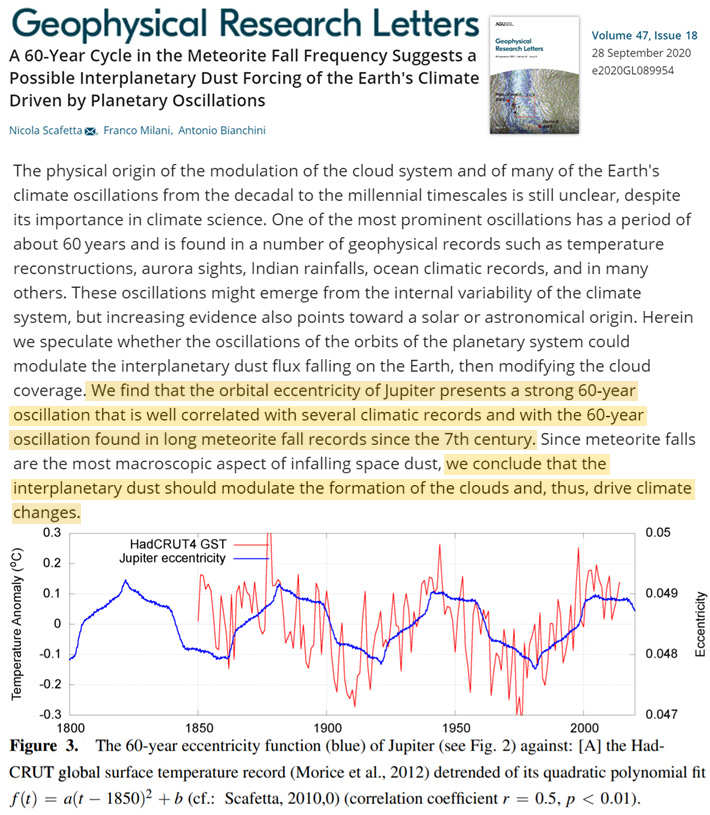
The physical origin of the modulation of the cloud system and of many of the Earth’s climate oscillations from the decadal to the millennial timescales is still unclear, despite its importance in climate science. One of the most prominent oscillations has a period of about 60 years and is found in a number of geophysical records such as temperature reconstructions, aurora sights, Indian rainfalls, ocean climatic records, and in many others. These oscillations might emerge from the internal variability of the climate system, but increasing evidence also points toward a solar or astronomical origin. Herein we speculate whether the oscillations of the orbits of the planetary system could modulate the interplanetary dust flux falling on the Earth, then modifying the cloud coverage. We find that the orbital eccentricity of Jupiter presents a strong 60‐year oscillation that is well correlated with several climatic records and with the 60‐year oscillation found in long meteorite fall records since the 7th century. Since meteorite falls are the most macroscopic aspect of infalling space dust, we conclude that the interplanetary dust should modulate the formation of the clouds and, thus, drive climate changes.
Much of the evidence for solar-climate interactions relies on model simulations and statistical analyses showing 11-year sunspot cycle variations in atmospheric circulation patterns (Gray et al., 2010; Matthes et al., 2017). This evidence reveals that supposedly small solar variations (on the order of one per mil for total solar irradiance −TSI−) may cause significant climatic responses driven by feedback mechanisms and internal climate variability that are not yet fully understood (Gray et al., 2010; Haigh, 1996; Lean, 1997; Matthes et al., 2003; Swingedouw et al., 2011).
Solar irradiance has been universally acknowledged to be dominant by quasi-decadal variability, which has been adopted frequently to investigate its effect on climate decadal variability. As one major terrestrial energy source, solar-wind energy flux into Earth’s magnetosphere (Em) exhibits dramatic interannual variation, the effect of which on Earth’s climate, however, has not drawn much attention. Based on the Em estimated by 3D magnetohydrodynamic simulations, we demonstrate a novelty that the annual mean Em can explain up to 25% total interannual variance of the northern-hemispheric temperature in the subsequent boreal winter.
These frequencies are also invariant relative to any spinning system centered on the Sun and, therefore, they and their combinations should characterize the spectrum of any forcing able to externally synchronizing the internal dynamics of the solar dynamo. Herein the orbital invariant inequalities of the solar system are determined and are demonstrated to cluster around specific spectral bands that exactly correspond to the above spectrum of solar activity. In particular, the orbital invariant inequality model is shown to predict, both in frequency and phase, the Bray-Hallstatt cycle (2100-2500 yr) found in ∆ 14C and in climate records throughout the Holocene. The result suggests that some kind of planetary forcing could be synchronizing solar internal dynamics.
[W]e show that increased frequency of upper‐level high PV events over western Europe is associated with enhanced blocking activity over eastern Europe. Therefore, the out of phase interannual to millennial‐scale variations of River Ammer flood frequency and solar irradiance, as presented in previous studies, can be explained by a solar modulation of eastern European‐western Russia summer blocking and associated upstream upper‐level wave breaking activity. In addition, we identify two distinct quasi‐periodic signals in both frequency of Lake Ammer flood layer and solar irradiance records with periods of ~900 years and ~2,300 years. We argue that similar cycles should dominate millennial‐scale variations of blocking activity in eastern Europe‐western Russia as well as extreme precipitation and flood frequency variability over central and western Europe during the last ~5,500 years.
The type-a circulation is typical for Grand Solar Maxima and is recorded at the known warm peaks at about AD ~970, ~1250, ~1320, ~1590 – 1600, ~1720 – 1790, and after 1900. The type-b and type-c circulations are typical for Grand Solar Minima and is well recorded and documented at the “little ice ages” around AD ~1050, ~1300, ~1450, ~1690, ~1810, and there are strong reasons to expect that it will re-occur at about AD 2040. … Grand Solar Maxima and Minima affect the Earth’s shielding capacity as a function of the Solar Wind interaction with the Earth’s geomagnetic field (e.g. [43]). The shielding controls the penetration of particles responsible for the formation of 14C in the atmosphere, the atmospheric 10Be content and cosmic ray particles [44]. The variations in atmospheric 14C content are well documented and provide a continual record of the variations in Solar Wind intensity and its effect on the Earth’s geomagnetic field strength as recorded by the changes in Earth’s shielding capacity. … In the period AD 900 – 1000, quite warm climatic conditions prevailed and there was a free sailing route from Iceland to Greenland. Already a century later icebergs and sea ice prevented a direct route to Greenland, and the sailing route was displaced to the south. This was just in the time of the Oort Grand Solar Minimum (Figure 4). By AD 1200 – 1400 the sailing route was even more displaced to the south, and the Viking settlements on Greenland were left to become extinct. Obviously, this was due to the cooling events during the Wolf and Spörer Grand Solar Minima. … Another important implication of Figure 9 scheme is that the solar impact on planet Earth primarily goes via heliomagnetic Solar Wind emission and not via total solar irradiance (TSI). When changes in the Earth’s geomagnetic shielding capacity are involved, we can be sure that the main forcing function comes from the Solar Wind interaction with the magnetosphere and the Earth’s rate of rotation (Figure 9). Therefore, observed variations in 14C and 10Be are the manifestation of changes in the shielding capacity (Solar Wind) not in TSI (as proposed by, for example, Bard et al. [61], Scafetta [1], and Veretenenko and Ogurtsov [101]). The so-called 60-yr cycle [102] must primarily be a function of heliomagnetic Solar Wind emission.
[T]he literature contains large discrepancies between estimates of solar forcing. For example, reconstructions of the increase of terrestrial solar irradiance (TSI) during the ETCW period [1921-1950] range from 0.6 Wm-2 (CMIP5, Wang et al., 2005), through 1.8 Wm-2 (Crowley et al., 2003), to 3.6 Wm-2 (Shapiro et al., 2011).
The role of natural factors, mainly solar 11-year cyclic variability and volcanic eruptions on two major modes of climate variability the North Atlantic Oscillation (NAO) and El Nin˜o Southern Oscillation (ENSO) are studied for about the last 150 years period. The NAO is the primary factor to regulate Central England Temperature (CET) during winter throughout the period, though NAO is impacted differently by other factors in various time periods. Solar variability during 1978–1997 indicates a strong positive in-phase connection with NAO, which is different in the period prior to that. Such connections were further explored by known existing mechanisms. Solar NAO lagged relationship is also shown not unequivocally maintained but sensitive to the chosen times of reference. It thus points towards the previously known mechanism/relationship related to the Sun and NAO. This study discussed the important roles played by ENSO on global temperature; while ENSO is influenced strongly by solar variability and volcanic eruptions in certain periods. A strong negative association between the Sun and ENSO is observed before the 1950s, which is positive though statistically insignificant during the second half of the twentieth century. The period 1978–1997, when two strong eruptions coincided with active years of strong solar cycles, the ENSO and volcano suggested a stronger association. That period showed warming in the central tropical Pacific while cooling in the North Atlantic with reference to various other anomaly periods. It indicates that the mean atmospheric state is important for understanding the connection between solar variability, the NAO and ENSO and associated mechanisms. It presents critical analyses to improve knowledge about major modes of variability and their roles in climate and reconciles various contradictory findings. It discusses the importance of detecting solar signal which needs to be robust too.
Comparison of these monsoon changes with solar activity and North Atlantic cooling events reveals that both factors can lead to abrupt changes on a centennial timescale in the Early Holocene. During the Late Holocene, North Atlantic cooling became the major forcing of centennial monsoon events.
Here, we extend the key mechanisms involving the oceanic Rossby waves in climate variability, to very long-period, multi-frequency Rossby waves winding around the subtropical gyres. Our study demonstrates that the climate system responds resonantly to solar and orbital forcing in eleven subharmonic modes. We advocate new hypotheses on the evolution of the past climate, implicating the deviation between forcing periods and natural periods according to the subharmonic modes, and the polar ice caps while challenging the role of the thermohaline circulation.
The Tibetan Plateau (TP), known as the world’s “Third Pole,” plays a vital role in regulating the regional and global climate and provides freshwater for about 1.5 billion people. Observations show an accelerated ground surface warming trend over the southeastern TP during the global warming slowdown period of 1998–2013, especially in the summer and winter seasons. The processes responsible for such acceleration are under debate as contributions from different radiative processes are still unknown. Here we estimate for the first time the contributions of each radiative component to the ground surface warming trend before and after 1998 by analyzing multisource datasets under an energy balance framework. Results show that declining cloud cover caused by the weakening of both the South Asian summer monsoon and local-scale atmospheric upward motion mainly led to the accelerated ground surface warming during the summers of 1998–2013, whereas the decreased surface albedo caused by the snow melting was the major warming factor in winter. Moreover, increased clear-sky longwave radiation induced by the warming middle and upper troposphere was the second largest factor, contributing to about 21%–48% of the ground surface warming trend in both the summer and winter seasons. … Previous work suggests that the cloud cover over the southern TP decreased during 1998–2009, which increased surface shortwave radiation and contributed to the continued warming over the TP (Duan and Xiao 2015) … multisource datasets suggest that cloud-radiative forcing and clear-sky longwave radiation are the main factors for the accelerated warming trend in summer.
A key characteristic of the anomaly series shown in Figure 3 is the inter-annual variability. It can be seen that the annual ground-based SIS time series exhibits a slight increase from 1985 to 1996, followed by a strong increase toward the end 1990s. From the early 2000s to 2015 there is another marked increase, which results on a significant positive linear trend over the entire study period 1985-2015 of +4.4±1.3 Wm-2 decade-1 (+2.6±0.8 % decade-1). This result agrees with the SIS [surface solar radiation] trends over the Iberian Peninsula since the 1980s (Sanchez-Lorenzo et al., 2013; Wild, 2009), as well as with the increasing sunshine duration in the 1980-2000 period reported by Sanchez-Lorenzo et al. (2007).
Here we bring together co-located long-term observational data from surface and space to study decadal changes of the shortwave energy balance in Europe and China from 1985 to 2015. Within this observation-based framework, we show that an increasing net shortwave radiation at the top of the atmosphere and a decreasing atmospheric shortwave absorption each contribute roughly half of the observed brightening trends in Europe. For China, we find that the continued dimming until 2005 and the subsequent brightening occurred despite opposing trends in the top-of-the-atmosphere net shortwave radiation. This shows that changes in atmospheric shortwave absorption are a major driver of European brightening and the dominant cause for the Chinese surface trends. Although the observed variations cannot be attributed unambiguously, we discuss potential causes for the observed changes.
ENSO, NAO, AMO, PDO Climate Influence
This study reveals a marked enhancement in the relationship between the North Atlantic Oscillation (NAO) and North Atlantic tripole (NAT) sea surface temperature (SST) anomaly pattern during boreal spring since the late 1980s. A comparative analysis is conducted for two periods before and after the late 1980s to understand the reasons for the above interdecadal change. During both periods, SST cooling in the northern tropical Atlantic during the positive phase of the NAT SST pattern results in an anomalous anticyclone over the subtropical western North Atlantic via a Rossby wave–type atmospheric response.
By analyzing the relationship between these investigated phenomena of mass changes from GRACE and SMB-D and NAO index, we were able to understand better the mechanism of how climate changes influence the GrIS mass. As seen in Figure 8, the negative phase of the summertime NAO (sNAO) index (June-July-August), such as in 2008 and 2012, increased the prevalence of high pressure, enhancing the surface absorption of solar radiation and decreasing precipitation. It caused the migration of warm air from southern latitudes into western Greenland. These changes promoted higher air temperatures, a longer ablation season, and enhanced melt and run-off. The positive phase of the sNAO index, such as in 2013, increased precipitation and decreased air temperatures, leading to a shorter ablation season and smaller mass loss. An increased mass loss has been related to increased occurrences of the negative phases of NAO during summer, which favors an anticyclonic circulation at upper levels and warmer conditions over Greenland at lower levels through the advection of warm air along its western coast. NAO is a large-scale climate driver, and it influences mass changes in Greenland by controlling regional temperature, precipitation, and atmospheric circulation.
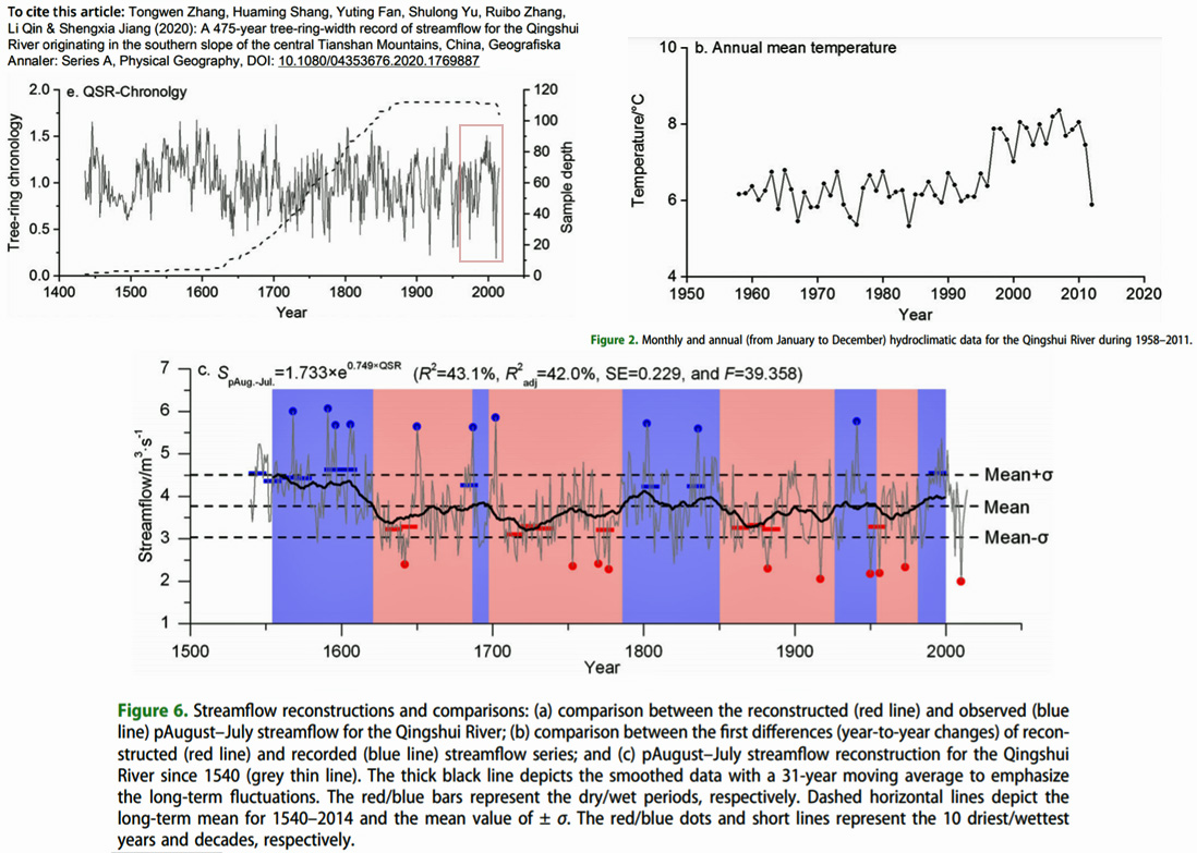
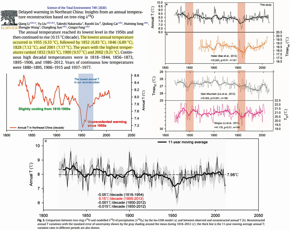
Annual T was regulated by the EASM and NAO during the past two centuries. … The annual temperature reached its lowest level in the 1950s and then continued to rise (0.15 °C/decade). The lowest annual temperature occurred in 1955 (6.33 °C), followed by 1852 (6.83 °C), 1846 (6.89 °C), 1828 (7.12 °C), and 2001 (7.17 °C). The years with the highest temperatures ranked 1832 (9.63 °C), 1900 (9.57 °C) and 2002 (9.21 °C). Continuous high decadal temperatures were in 1818–1844, 1856–1873, 1895–1906, and 1986–2012. Years of continuous low temperatures were 1880–1895, 1906–1915 and 1937–1977.
The El Niño-Southern Oscillation (ENSO) is a major driver of global climate variability. The ENSO also interacts with other modes of climate variability, such as the Indian summer monsoon rainfall (ISMR). The easterly trade winds and SST gradients across the equatorial Pacific undergo a regime change, with enhanced trade winds and significant cooling (warming) over the tropical eastern (western) Pacific in the later period. Previous research has shown that the relationship between the ISRM and SSTs is variable. The strongest relationships were found on short timescales (interdecadal periodicity, 2–7 years) or decadal periodicity (10.5 years) but with varying significance levels. Several studies have examined the relationships between the ISM and ENSO phenomenon and/or variations in SST and sea surface pressure (SSP) in the Pacific Ocean. This result suggests that δ18Otr records multiple ENSO phenomena. Several studies have pointed to the fact that the influence of the ENSO phenomenon on the ASM varies over time
The Southern Annular Mode (SAM) is the leading mode of extratropical Southern Hemisphere climate variability, associated with changes in the strength and position of the polar jet around Antarctica. This variability in the polar jet drives large fluctuations in the Southern Hemisphere climate, from the lower stratosphere into the troposphere, and stretching from the midlatitudes across the Southern Ocean to Antarctica. Notably, the SAM index has displayed marked positive trends in the austral summer season (stronger and poleward shifted westerlies), associated with stratospheric ozone loss. Historical reconstructions demonstrate that these recent positive SAM index values are unprecedented in the last millennia, and fall outside the range of natural climate variability. Despite these advances in the understanding of the SAM behavior, several areas of active research are identified that highlight gaps in our present knowledge.
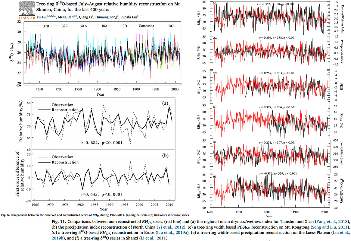
Based on the above analyses, ENSO has the largest effect on the intensity of the ASM [Asian summer monsoon], followed by the solar activity and NAO (Wang,2006; Wang et al., 2013). This process is finally recorded by the treering δ18O values in the Mt. Shimen region. The reconstruction is significantly positively correlated with several Asian summer monsoon (ASM) indices, indicating that the reconstructed RHJA reflects the variations in ASM intensity to a large extent. In terms of the local climate change mechanisms, we found that the factors affecting the variations in RHJA in the Mt. Shimen region are complex and involve large-scale oceanic–atmospheric couplings, such as sea surface temperature (SST), El Niño-Southern Oscillation (ENSO) and North Atlantic Oscillation (NAO). Solar activity also certainly has great impacts.
Over the last two and a half centuries, the region has experienced six warm periods, namely 1766–1792, 1803–1827, 1878–1886, 1904–1916, 1926–1935, and 1982–2015. The reconstruction also indicates the occurrence of two significant cold periods, 1821-1857 and 1931–1980. Over the past 252 years, the climate in this region has shifted between warm-dry and cold-wet periods. However, a strong warm-wet trend since the 1980s is evident. There is a strong positive correlation between the tree-ring temperature reconstruction and the North Atlantic Oscillation, as well as a close relationship with strong volcanic eruptions in the mid-high latitudes.
Previous studies have shown that the aforementioned variabilities of Arctic sea ice, Eurasian snow, and ENSO are closely linked with each other, although the mechanisms of the underlying connections are complex. Recent studies have suggested a similar chain of events from boreal autumn to winter for both snow cover and sea ice (Cohen et al., 2014; Wegmann et al., 2015; Gastineau et al., 2017). Arctic sea ice changes can occur independently but sometimes co-occur with ENSO. For example, substantially less sea ice occurred in 2007 autumn, which was followed by a strong La Niña event in the subsequent winter. More sea ice appeared in 1997 autumn, which was accompanied by a strong El Niño in the following winter. Ding et al. (2014) suggested that their observations and model experiments showed that the central tropical Pacific SST may affect the recent Arctic warming over northeastern Canada and Greenland through Rossby wave propagation. The cooling trend over equatorial Pacific is strongly coupled with winter sea ice melting in the Barents Sea and anticyclone formation over Scandinavia (Dobricic et al., 2016).
Climate/Precipitation Natural Variability
The main purpose of this study was to assess how internal variability has influenced GrIS changes, and what modes of atmospheric variability matter most for GrIS melting patterns. We find that internal variability dominates the forced signal associated with GrIS melt on short timescales (roughly 15 years in southwest Greenland and up to 30 years in the northwest) and that this internal variability expands into the interior of the GrIS as temperatures increase in the future. These results suggest that internal variability plays a role in ice sheet changes and that a greater area of the GrIS will be susceptible to internal variability as anthropogenic climate change induces further warming. Through the implementation of maximum covariance analysis, we determined the dominant modes of covariability between internal atmospheric circulation variability and conditions conducive to ice melt over Greenland. From our analysis, we found that a large portion of the melt variability (>54%) can be explained by the North Atlantic Oscillation, corresponding to the first EOF of the SLP variability.
The surface air temperature (SAT) exhibits pronounced warming over West Antarctica in recent decades, especially in austral spring and winter. Using a 30-member ensemble of simulations by Community Earth System Model (CESM), two reanalysis datasets, and observed station data, this study investigates the relative contributions of internally generated low-frequency climate variability and externally forced climate change to the austral winter SAT trend in Antarctica. Although these simulations share the same external forcing, the SAT trends during 1979–2005 show large diversity among the individual members in the CESM ensemble simulations, suggesting that internally generated variability contributes a considerable part to the multidecadal SAT change in Antarctica. Quantitatively, the total forced contribution to the SAT (1979–2005) change is about 0.53 k/27 yr, and the internal variability can be strong enough to double or cancel the externally forced warming trend. A method called “dynamical adjustment” is utilized to further divide the forced response. We fnd both the forced thermodynamically-induced and the forced dynamically-induced SAT trends are positive over all the regions in Antarctica, with the regional mean values of 0.20 k /27 yr and 0.33 k/27 yr, respectively. The diversity of SAT trends among the simulations is closely linked to a Southern hemisphere Annular Mode (SAM)-like atmospheric circulation multidecadal change in the Southern Hemisphere. When there exists a positive–negative seesaw of pressure trend between Antarctica and the mid-latitudes, the SAT trend is positive over most of Antarctica but negative over the Antarctic Peninsula, and vice versa. The SAM-like atmospheric circulation multidecadal change mainly arises from atmospheric internal variability rather than remote tropical Sea Surface Temperature (SST).
We present the first multi-century, annual-resolution record of snowpack variability for southwestern BC based on tree-ring width data from PSF and MH trees. Our reconstruction portrays regionally relevant snowpack patterns, differences in variability, and the influence of ENSO on snowpack variability during the instrumental period. It also shows that in the past, snow droughts were up to twice as long duration and twice as severe in magnitude than snow droughts in the observed record. Importantly, these past and more severe snow droughts represent long-term natural variability in the snowpack system and were not additionally influenced by anthropogenic climate change. Wavelet analysis suggests our reconstruction may also capture the influence of Pacific Ocean oscillations across the full reconstructed period. The reconstruction highlights the potential for developing pre-instrumental annual and/or seasonal snowpack records in BC that are relevant for developing water management policies.
A remarkable signature of the climate of the past 100 kyrs are the so called Dansgaard-Oeschger (DO) events (Dansgaard et al., 1984). These events occurred during the last glacial period and are characterised by abrupt warming within a few decades of 5-10 degrees followed by more gradual cooling over more than 1 kyr back to the stadial period with DO events recurring on average every 1470 years. … The apparent regularity in the temporal spacing between successive Dansgaard-Oeschger events, which has been determined from ice-core data to be roughly 1470 years, is here not caused by any inherent periodicity in the system but rather by the random occurrence of extreme sea-ice extents above a certain threshold below which the response of the ocean is not significant. This is in accordance with Ditlevsen et al. (2007) who showed that there is no statistically significant evidence for strict periodicity.
The Indian Ocean Dipole (IOD) affects climate and rainfall across the world, and most severely in nations surrounding the Indian Ocean. The frequency and intensity of positive IOD events increased during the twentieth century and may continue to intensify in a warming world. However, confidence in predictions of future IOD change is limited by known biases in IOD models and the lack of information on natural IOD variability before anthropogenic climate change. Here we use precisely dated and highly resolved coral records from the eastern equatorial Indian Ocean, where the signature of IOD variability is strong and unambiguous, to produce a semi-continuous reconstruction of IOD variability that covers five centuries of the last millennium. Our reconstruction demonstrates that extreme positive IOD events were rare before 1960. However, the most extreme event on record (1997) is not unprecedented, because at least one event that was approximately 27 to 42 per cent larger occurred naturally during the seventeenth century.
Recent Antarctic surface climate change has been characterized by greater warming trends in West Antarctica than in East Antarctica. Although this asymmetric feature is well recognized, its origin remains poorly understood. Here, by analyzing observation data and multimodel results, we show that a west-east asymmetric internal mode amplified in austral winter originates from the harmony of the atmosphere-ocean coupled feedback off West Antarctica and the Antarctic terrain. The warmer ocean temperature over the West Antarctic sector has positive feedback, with an anomalous upper-tropospheric anticyclonic circulation response centered over West Antarctica, in which the strength of the feedback is controlled by the Antarctic topographic layout and the annual cycle. The current west-east asymmetry of Antarctic surface climate change is undoubtedly of natural origin because no external factors (e.g., orbital or anthropogenic factors) contribute to the asymmetric mode.
The study area experienced four dry periods (precipitation below average): 1895–1900, 1920–1944, 1984–1994 and 2011–2016 during the past 122 a. The driest period was 1920–1944, with the monthly mean SPEI value being 0.24 below the average of 1895–2016. The longest dry period lasted for 25 a (1920–1944; Table 3). During the past 122 a, the study area also experienced three wet periods (precipitation above average): 1901–1919, 1945–1983 and 1995–2010. The wettest period was 1901–1919, with the monthly mean SPEI value being 0.52 above the average of 1895–2016. … Evidence from the reconstruction of precipitation changes at Taibai Mountain in the Qinling Mountains and the reconstruction of temporal and spatial precipitation changes in the middle and eastern part of Northwest China over the past 400 a showed that the drought was most obvious from the 1920s to 1930s (Li et al., 2012; Liu, 2016).
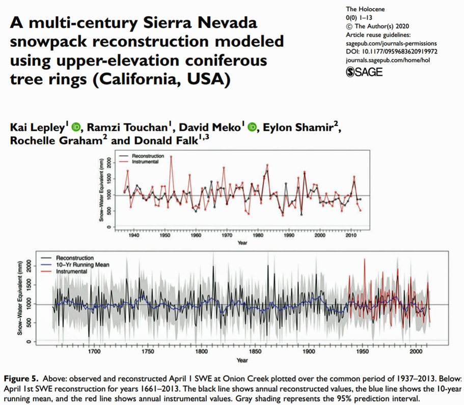
The results of this study demonstrate the effectiveness of using tree-rings to inform past climate while highlighting points of discretion. Specifically, SWE [snow water equivalent] is skillfully reconstructed using high-elevation coniferous tree rings in a central watershed of the Sierra Nevada mountains of California.
Huerta and Lavado-Casimiro, 2020
The results indicate that there is no significant global trend towards wet or dry conditions in the PA, although a signal of a more slightly decrease of precipitation is presented in the Southern PA. Additionally, interannual variability of total precipitation is mainly dominated by precipitation frequency. The Central Tropical Pacific sea surface temperature plays a major role for the maximum and average length of wet periods as well as for total precipitation.
Using a worldwide database that extends over almost the entire period of significant anthropogenic emission of greenhouse gases, we have found, in every region for which we have enough data for significant results, a statistically significant mean decreasing trend in aridity. … Our results disagree with the hypothesis that drier regions are getting drier. In all regions except South America there is no evident correlation between aridity and its rate of change. In South America the wetter sites are rapidly increasing in wetness, but the drier sites are not, on average, getting significantly drier, although there is substantial apparent random scatter.
[W]e show that even out to thirty years large parts of the globe (or most of the globe in MPI-GE and CMIP5) could still experience no-warming due to internal variability. … We first confirm that on short-term time-scales (15-years) temperature trends are dominated by internal variability. This result is shown to be remarkably robust. There is near-equivalence between the six individual SMILEs and CMIP5, demonstrating that the SMILE results hold when using all available climate models. We find that internal variability dominates projections even when we take the smallest estimate of internal variability available from the SMILEs. … Second we confirm that on mid-term time-scales (30-years) internal variability is still important for driving temperature trends, however in this case both structural model differences and scenario (or pathway) uncertainty also matter, with model differences having the greater importance of the two.
Cloud Climate Influence
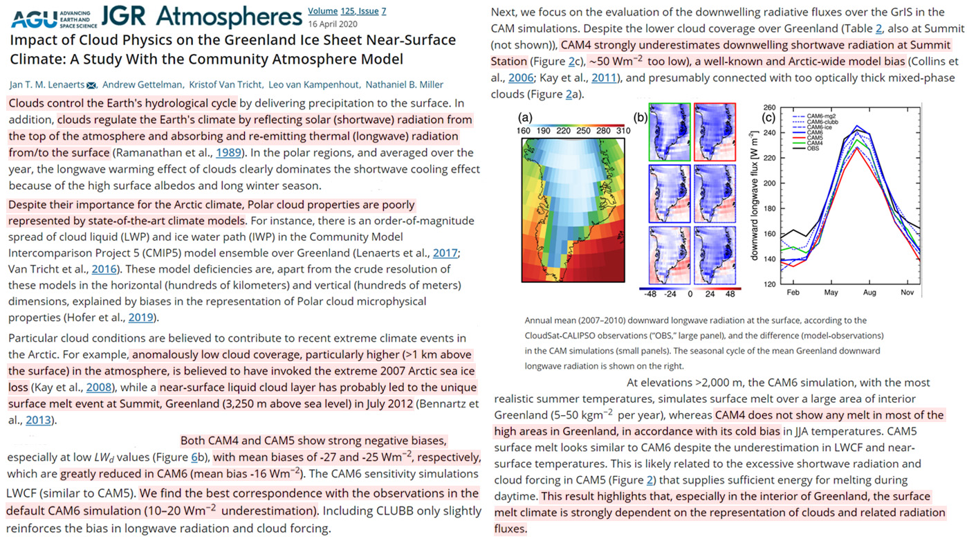
Clouds control the Earth’s hydrological cycle by delivering precipitation to the surface. In addition, clouds regulate the Earth’s climate by reflecting solar (shortwave) radiation from the top of the atmosphere and absorbing and re‐emitting thermal (longwave) radiation from/to the surface (Ramanathan et al., 1989). … Particular cloud conditions are believed to contribute to recent extreme climate events in the Arctic. For example, anomalously low cloud coverage, particularly higher (>1 km above the surface) in the atmosphere, is believed to have invoked the extreme 2007 Arctic sea ice loss (Kay et al., 2008), while a near‐surface liquid cloud layer has probably led to the unique surface melt event at Summit, Greenland (3,250 m above sea level) in July 2012 (Bennartz et al., 2013). … Despite their importance for the Arctic climate, Polar cloud properties are poorly represented by state‐of‐the‐art climate models. For instance, there is an order‐of‐magnitude spread of cloud liquid (LWP) and ice water path (IWP) in the Community Model Intercomparison Project 5 (CMIP5) model ensemble over Greenland (Lenaerts et al., 2017; Van Tricht et al., 2016). … Both CAM5 and CAM6 indicate higher ice cloud cover frequencies over the western GrIS but fail to simulate the observed patterns in great detail. In agreement with the observations, both models show a higher ice cloud cover frequency (20%–30%) over the interior ice sheet than along the periphery. However, both models suggest that these clouds exist all the way to the surface, while the observations show a clear decrease in cloud cover frequency going from 1 km above the surface downward. … CAM4 strongly underestimates downwelling shortwave radiation at Summit Station (Figure 2c), ∼50 Wm−2 too low), a well‐known and Arctic‐wide model bias (Collins et al., 2006; Kay et al., 2011), and presumably connected with too optically thick mixed‐phase clouds (Figure 2a). … Both CAM4 and CAM5 show strong negative biases, especially at low LWd values (Figure 6b), with mean biases of ‐27 and ‐25 Wm−2, respectively, which are greatly reduced in CAM6 (mean bias ‐16 Wm−2). The CAM6 sensitivity simulations (not shown) show similar behavior than reported in Figure 5. … At elevations >2,000 m, the CAM6 simulation, with the most realistic summer temperatures, simulates surface melt over a large area of interior Greenland (5–50 kgm−2 per year), whereas CAM4 does not show any melt in most of the high areas in Greenland, in accordance with its cold bias in JJA temperatures. CAM5 surface melt looks similar to CAM6 despite the underestimation in LWCF and near‐surface temperatures. This is likely related to the excessive shortwave radiation and cloud forcing in CAM5 (Figure 2) that supplies sufficient energy for melting during daytime. This result highlights that, especially in the interior of Greenland, the surface melt climate is strongly dependent on the representation of clouds and related radiation fluxes.
Surface melting on Antarctic Peninsula ice shelves can influence ice shelf mass balance, and consequently sea level rise. We show that summertime cloud phase on the Larsen C ice shelf on the Antarctic Peninsula strongly influences the amount of radiation received at the surface and can determine whether or not melting occurs.
It is long established that CREs [cloud radiative effects] play a central role in determining Earth’s mean climate. It is becoming increasingly clear that they also play a key role in Earth’s climate variability across a range of time scales. In two recent studies, Rädel et al. (2016) and Middlemas et al. (2019) argue that the inclusion of coupling between the atmospheric circulation and clouds projects onto the variance of the ENSO, primarily due to the projection of longwave or shortwave CREs onto ENSO physics. Here we argue that coupling between the atmospheric circulation and CREs leads to a much broader and more basic effect on the climate system: Cloud circulation coupling leads to increases in the variance of SSTs on time scales from months to decades that are apparent throughout the tropical oceans (Figs. 1c, 2) and cannot be explained as the linear response to simulated ENSO variability.
The clouds represent a key element within the terrestrial climate system. In fact, clouds may be the most important parameter controlling the radiation budget, and, hence, the Earth climate (Hughes, 1983). This is related to the fact that clouds have a paramount importance in the radiation balance at global scale, especially due to their albedo (Ohring and Clapp, 1980). … Chiacchio and Wild (2010) have shown that more positive NAO during 1985–2000 is linked with the increase of solar radiation in Europe due to lower amounts of cloud cover which are characteristic for the southern part of the continent during positive NAO. They showed that NAO, generally anticorrelated with cloud cover at continental scale, represents one of the most important drivers of changes in solar radiation in Europe. Sfîcă et al. (2017) found that higher values of sunshine duration during winter in Romania are linked with an intense westerly circulation at continental scale. This supports the idea that there is an important link between atmospheric circulation and cloud cover. The effect on surface radiation of the decrease in cloud cover adds to the observed decrease of the optical thickness of aerosols leading to the so‐called brightening period during the last decennia (Russak, 2009; Pfeifroth et al., 2018a).
High-altitude cirrus clouds are climatically important: their formation freeze-dries air ascending to the stratosphere to its final value, and their radiative impact is disproportionately large.
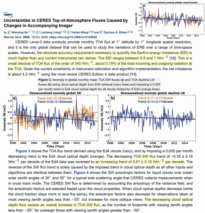
[A] 13% change in cloud optical depth results in about 1% change in the SW flux. … CERES…is the only global dataset that can be used to study the variations of ERB [Earth’s radiation budget] over a range of time-space scales. However, the absolute accuracy requirement necessary to quantify the Earth‘s energy imbalance (EEI) is much higher than any current instruments can deliver. The EEI ranges between 0.5 and 1 Wm−2 [12]. This is a small residual of TOA flux of the order of 340 Wm−2, about 0.15% of the total incoming and outgoing radiation at the TOA. Given the current uncertainty in instrument calibration and algorithm implementation, the net imbalance is about 4.3 Wm−2 using the most recent CERES Edition 4 data product [13].
Tropical convective clouds and the associated precipitation are essential modulators of the climate system. Given their significant contribution to the energy balance and the close connections to the hydrological cycle, modulation of clouds and precipitation, including the coverage, frequency of occurrence, and optical and microphysical properties, can lead to substantial climate feedbacks … By using the direct observations of the vertical cloud structure, these studies can depict a progression of cloud types through the entire MJO lifecycle. With varying cloud profiles, the details of cloud physics in terms of radiative heating, cloud-water enhancement, and related moist physics have proven that cloud plays a crucial role in the atmospheric radiative transfer processes during the active and suppressed phases of the MJO.
Clouds over the Southern Ocean (SO) differ from those over the Northern Hemisphere oceans, with low-altitude supercool clouds being more ubiquitous over the SO (Mace et al. 2009, 2010; Huang et al. 2016). Global climate model simulations (Trenberth and Fasullo 2010) and reanalysis products (Naud et al. 2014) struggle to represent these clouds, and in recent years, a lack of low cloud over the Southern Ocean, primarily in the cold sector of cyclonic systems, has been found to result in large radiative errors in both climate models and reanalysis (Williams et al. 2013, Naud et al. 2014, Bodas-Salcedo et al. 2014, 2016; Kay et al 2016). These cloud radiative errors result in significant errors in the surface energy budget and excess heat uptake by the ocean surface (Sallée et al. 2013, Schneider and Reusch 2016), and are of profound importance to global climate, including influencing the position of the Southern Hemisphere midlatitude jet, the Intertropical Convergence Zone position, cross-hemispheric energy transports (Ceppi et al. 2012, 2013; Hwang and Frierson 2013, Kay et al 2016), and even SO cloud feedbacks and global climate sensitivity (Gettelman et al 2019b, Bodas-Salcedo et al. 2019).
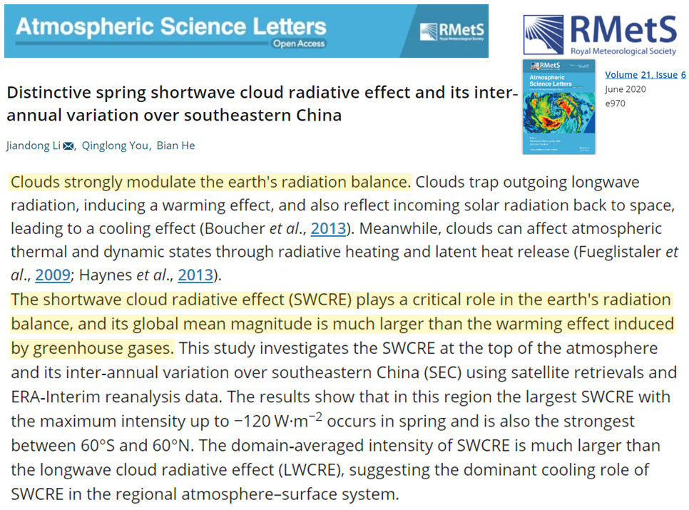
The shortwave cloud radiative effect (SWCRE) plays a critical role in the earth’s radiation balance, and its global mean magnitude is much larger than the warming effect induced by greenhouse gases. … Clouds strongly modulate the earth’s radiation balance. Clouds trap outgoing longwave radiation, inducing a warming effect, and also reflect incoming solar radiation back to space, leading to a cooling effect (Boucher et al., 2013).
Cloud radiative effects (CREs) are known to play a central role in governing the long-term mean distribution of sea-surface temperatures (SSTs). Very recent work suggests that CREs may also play a role in governing the variability of SSTs in the context of the El Niño/Southern Oscillation.
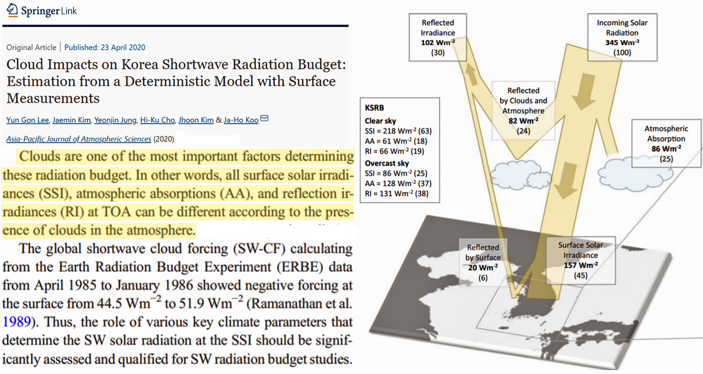
Clouds are one of the most important factors determining the radiation budget. In other words, all surface solar irradiances (SSI), atmospheric absorptions (AA), and reflection irradiances (RI) at TOA can be different according to the presence of clouds in the atmosphere. … The global shortwave cloud forcing (SW-CF) calculating from the Earth Radiation Budget Experiment (ERBE) data from April 1985 to January 1986 showed negative forcing at the surface from 44.5 Wm−2 to 51.9 Wm−2 (Ramanathan et al. 1989). Thus, the role of various key climate parameters that determine the SW solar radiation at the SSI should be significantly assessed and qualified for SW radiation budget studies. … Clouds in all- (or overcast-) sky atmosphere diminish surface solar irradiances (SSI) from 218.1 Wm−2 to 156.9 Wm−2 (or 85.8 Wm−2) and enhance atmospheric absorptions (AA) from 61.5 Wm−2 to 86.3 Wm−2 (or 128.2 Wm−2). Clouds also enhance the reflected irradiances (RI) at the TOA from 65.6 Wm−2 to 102.0 Wm−2 (or 131.2 Wm−2) for all- (or overcast-) skies. As a result, the all- (or overcast-) sky shortwave (SW) cloud forcing (CF) is −61.2 Wm−2 (or −132.3 Wm−2) at the surface, AA is 24.8 Wm−2 (or 66.7 Wm−2) in the atmosphere and RI is 36.4 Wm−2 (or 65.6 Wm−2) at the TOA, respectively.
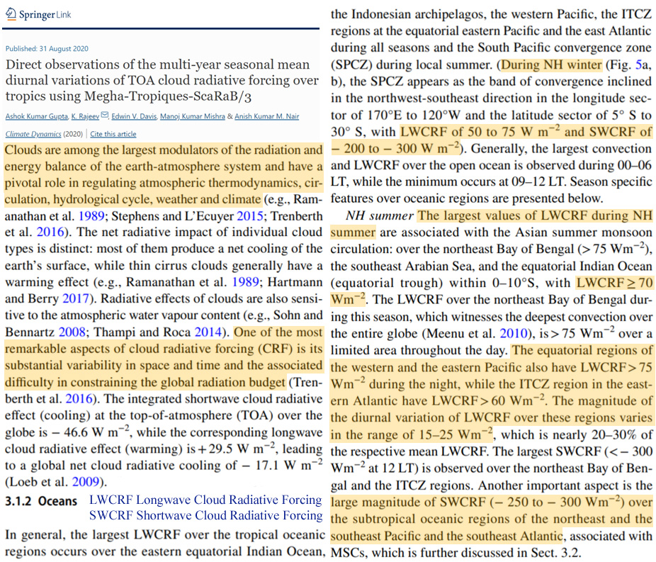
Diurnal variation of cloud radiative forcing (CRF) is a major factor that controls the global radiation balance. … Clouds are among the largest modulators of the radiation and energy balance of the earth-atmosphere system and have a pivotal role in regulating atmospheric thermodynamics, circulation, hydrological cycle, weather and climate (e.g., Ramanathan et al. 1989; Stephens and L’Ecuyer 2015; Trenberth et al. 2016).
In this study, we use CERES observations to evaluate how state‐of‐the‐art climate models represent changes in Earth’s radiation budget following a large change in SST patterns. The CERES data reveal a 0.83 Wm−2 reduction in global mean reflected shortwave (SW) flux during the 3 years following the hiatus, resulting in an increase in net energy into the climate system (Loeb, Thorsen, et al., 2018). Furthermore, decreases in low‐cloud cover are found to be the primary driver of the decrease in SW flux. The low‐cloud cover decreases are associated with increases in SST reaching 2 °C on average in some locations over the eastern Pacific Ocean following a change in the sign of the Pacific Decadal Oscillation from negative to positive phase. … The SW flux decrease with SST off the west coast of North America is qualitatively consistent with other satellite studies that found a negative correlation between low‐cloud cover and SST from passive (McCoy et al., 2017; Myers & Norris, 2015; Qu et al., 2015; Yuan et al., 2018) and active sensors (Cesana et al., 2019; Myers & Norris, 2015). … Over longer timescales, coupled climate model simulations also suggest an important role for low clouds in determining the future climate state.
It is possible that DCC [daily cloud cycle] variations adjust the Earth’s energy balance and partially contribute to the phenomenon of climate hiatus. Our application to climate model outputs shows that large intermodel spread of DCCRE, seldom been considered in climate model assessment, turns out to be a nonnegligible part of CRE [cloud radiative effects] inter-model variations. … Satellite observations show that the daily cloud cycle is strongly linked to pacific decadal oscillation (PDO) and climate hiatus, revealing its potential role in controlling climate variability. … [T]he variations of DCC [daily cloud cycle] may partially control the global surface temperature and the inter-model spread of DCC radiative impacts accounts for approximately 20% spread of the CRE in climate models, highlighting the importance of this specific cloud property.
Clouds crucially regulate atmospheric energy balance, water circulation, and Earth’s climate system with multiple spatiotemporal scales (Boucher et al. 2013). Fundamental conundrums on clouds, the coupling of clouds with atmospheric circulation, and climate interactions have remained unsolved and have been identified as considerable challenges in climate research (Bony et al. 2015). One of the largest uncertainties amongst these challenges is the vertical property of clouds and their radiative effects (Li et al. 2015). Vertical variation of clouds can affect the vertical distribution of atmospheric radiative heating, surface energy balance, and general circulation by changing the vertical structure of radiative warming and cooling rates (Johansson et al. 2015; Pan et al. 2017). Quantifying the vertical distribution of cloud radiative forcing and their impacts on atmospheric circulation and regional climate has become critical.
Clouds are centrally important in climate studies to understand the radiative energy budget of the Earth’s atmosphere system, hydrological cycle, and precipitation. For example, low-level clouds play a crucial role in the radiation budget of the Earth by modulating the shortwave cloud radiative forcing, and high clouds play a vital role in the radiation budget by modulating the longwave cloud radiative forcing. However, their proper representation in GCMs has been an unresolved issue
Clouds control the Earth’s hydrological cycle by delivering precipitation to the surface. In addition, clouds regulate the Earth’s climate by reflecting solar (shortwave) radiation from the top of the atmosphere and absorbing and re-emitting thermal (longwave) radiation from/to the surface (Ramanathan et al., 1989). In the polar regions, and averaged over the year, the longwave warming effect of clouds clearly dominates the shortwave cooling effect because of the high surface albedos and long winter season. However, the cloud radiational effect varies substantially spatially and across seasons; for example, the cloud shortwave cooling effect dominates during the melt season, acting to reduce surface melting overall (Hofer et al., 2017; Niwano et al., 2019; Ruan et al., 2019; Wang et al., 2018, 2019). Cloud cover frequency, structure, and phase all are important for determining the extent of cloud warming (Shupe et al., 2004); while, in general, cold and high clouds preferentially dim shortwave radiation, low-level and liquid-containing also tend to absorb longwave radiation. Particular cloud conditions are believed to contribute to recent extreme climate events in the Arctic. For example, anomalously low cloud coverage, particularly higher (>1 km above the surface) in the atmosphere, is believed to have invoked the extreme 2007 Arctic sea ice loss (Kay et al., 2008), while a near-surface liquid cloud layer has probably led to the unique surface melt event at Summit, Greenland (3,250 m above sea level) in July 2012 (Bennartz et al., 2013).
The total mass of the atmosphere [or equivalently, the background surface pressure (SP)] may have varied significantly over the evolutionary histories of Earth and other planets. Atmospheric mass can affect climate by modifying physical processes, including shortwave scattering, the emissivity of greenhouse gases, the atmospheric heat capacity, and surface fluxes. We apply a three-dimensional global climate model to explore the dependence of climate on SP over the range of 0.5–2.5 bar. Our simulations show an intriguing, nonmonotonic dependence of climate on SP. Over the SP range of 0.5–0.9 and 1.5–2.5 bar, the surface temperature increases with SP; however, over the SP range of 0.9–1.5 bar, the surface temperature decreases with SP. The negative correlation is due to a convection–circulation–cloud coupled feedback. As SP increases, the moist adiabatic lapse rate increases, leading to upper-troposphere cold anomalies in the tropics and middle latitudes that increase the midlatitude baroclinicity and eddy activity. … Our results demonstrate that the regime transition of flow state (e.g., the merge of jets here) may induce large anomalies in clouds and radiative forcing, resulting in nonlinear climate responses.
Tropical high clouds play a central role in climate via their influences on the radiation budget, altering both the reflection of incoming solar radiation and the atmospheric absorption of long-wave radiation emitted by Earth’s surface (Trenberth et al., 2009; Dessler, 2010). The net effect of an individual cloud on the radiation budget depends on several factors, including the type, phase, height, and microphysical characteristics of the cloud (Stevens and Schwartz, 2012). These features are difficult to parameterize so that the integrated radiative impacts of clouds remain poorly represented in global models (Bony et al., 2015), including those used to produce atmospheric reanalyses (Dolinar et al., 2016; Li et al., 2017).
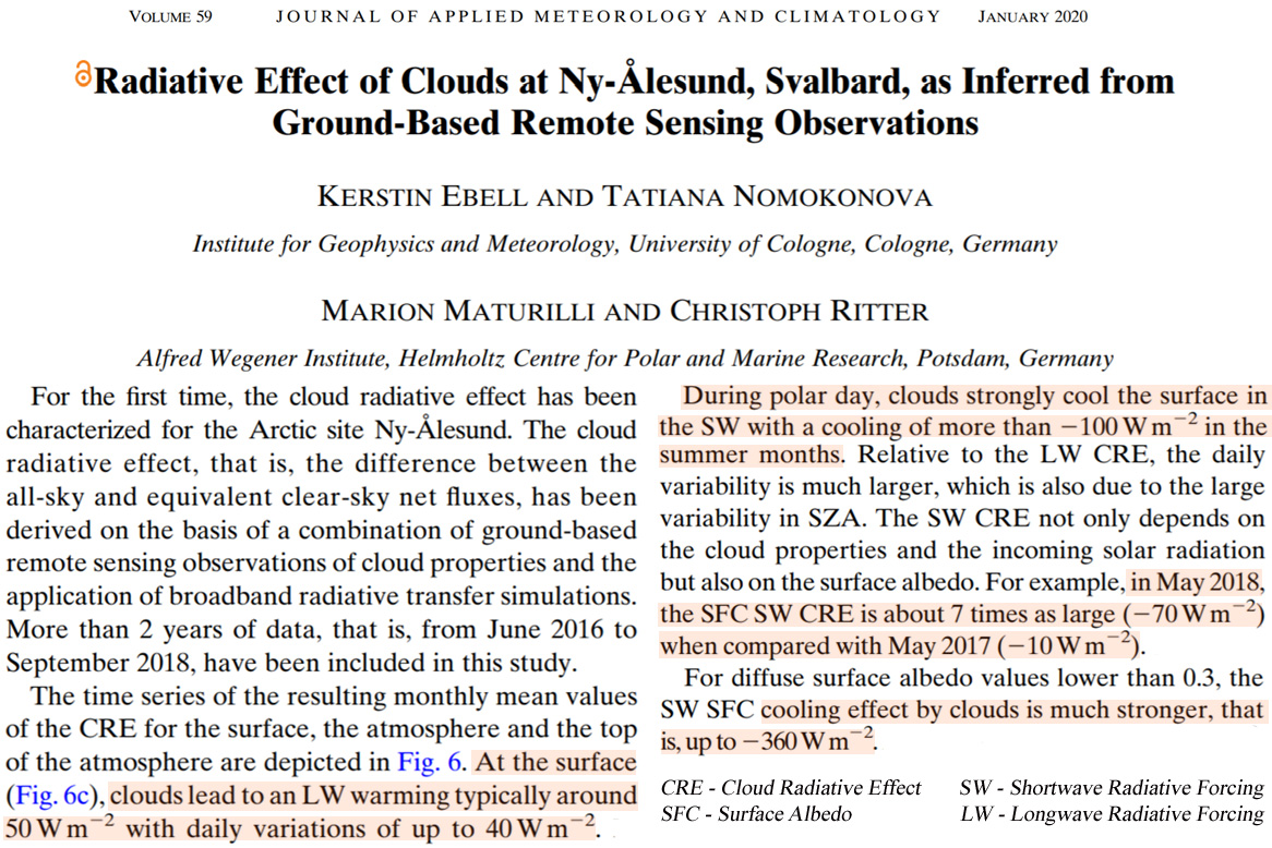
The time series of the resulting monthly mean values of the CRE for the surface, the atmosphere and the top of the atmosphere are depicted in Fig. 6. At the surface (Fig. 6c), clouds lead to an LW warming typically around 50 W/m² with daily variations of up to 40 W/m² … During polar day, clouds strongly cool the surface in the SW with a cooling of more than 100 W/m² in the summer months. Relative to the LW CRE, the daily variability is much larger, which is also due to the large variability in SZA. The SW CRE not only depends on the cloud properties and the incoming solar radiation but also on the surface albedo. For example, in May 2018, the SFC SW CRE [surface albedo shortwave cloud radiative effect] is about 7 times as large (70 W/m²) when compared with May 2017 (10 W/m²).
Toward this goal, here we analyze the radiation at the top of the atmosphere and propose a measure of the DCC [diurnal cloud cycle] radiative effect (DCCRE) as the difference between the total radiative fluxes with the full cloud cycle and its uniformly distributed cloud counterpart. When applied to the frequency of cloud occurrence, DCCRE is linked to the covariance between DCC and cloud radiative effects. Satellite observations show that the daily cloud cycle is strongly linked to pacific decadal oscillation (PDO) and climate hiatus, revealing its potential role in controlling climate variability.
The CO2 Greenhouse Effect – Climate Driver?
Zhang et al., 2020 (full paper)
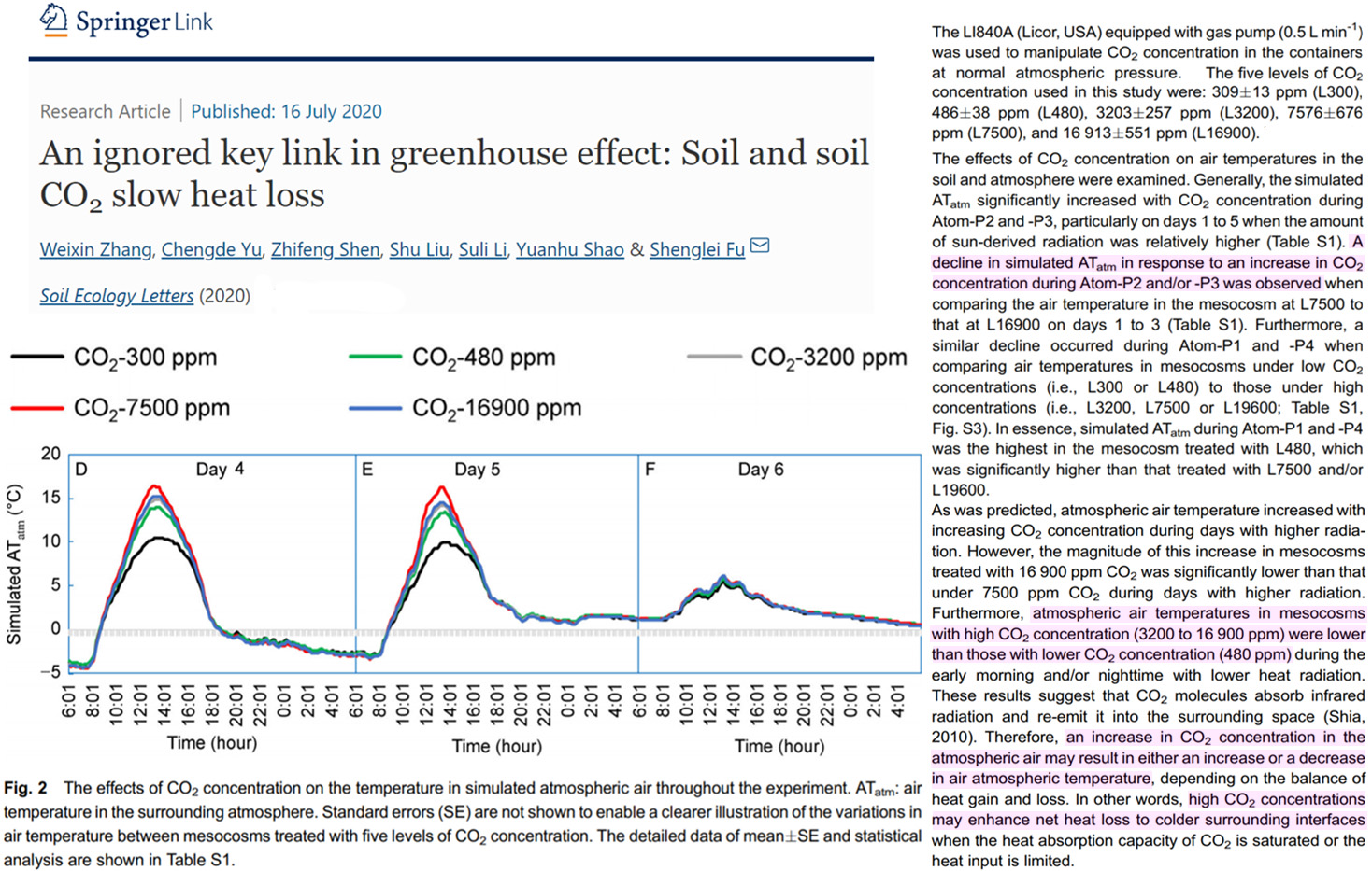
The increased atmospheric air temperatures with CO2 concentration (ranging from 300 ppm to 7500 ppm) at daytime with higher radiation were understandable. Unexpectedly, the magnitude of temperature increase of atmospheric air in mesocosms with 16900 ppm CO2 declined significantly compared to that with 7500 ppm CO2 at daytime with higher radiation. In addition, the temperatures of atmospheric air in mesocosms with substantially higher CO2 concentration (ranging from 3200 ppm to 16900 ppm) were lower than that with the lower CO2 concentration (480 ppm) at early morning and/or nighttime with lower heat radiation. These results emphasized that the molecules of CO2 not only absorb the infrared radiation but also re-emit it to the surrounding space (20). Thus an increase of CO2 concentration in atmospheric air may result in either an increase or decrease of the air temperature in the atmosphere, depending on the balance of heat gain and loss. In other words, CO2 with substantially higher concentration may enhance the net heat loss to colder surrounding interfaces when the heat absorption capacity of CO2 was saturated or heat input was much limited. … [T]he significant decrease of soil air temperature in mesocosms with CO2 concentration of 16900 ppm indicated that soil with substantially higher CO2 concentration may cool the soil probably by transferring more heat to surrounding space during colder periods when the temperature difference between soil and surface atmospheric air became larger. The realistic significance of these findings was greater than those in the atmosphere because CO2 concentration in soil air was often in the range of 1,000 ppm – 20,000 ppm [21-23]. Hence, the variation of soil CO2 concentration may regulate the balance of heat gain and loss in soil which determines the contribution of soil to surface warming of the earth.
Although the long-term (climatological) mean properties of the equilibrium response vary smoothly as a function of the CO2 concentration, a change in the nature of variability introduces strong nonlinearity in the response at high concentrations. In particular, the climatological mean value of the global mean surface temperature practically stops responding to an increase in the CO2 concentration. This practically zero climate sensitivity suggests that the effect of a feedback on the global mean surface temperature may turn out to be as strong as the radiative effect of CO2, even if the feedback varies smoothly and monotonically and is well-behaved in general. This may be regarded as a warning that even “first estimates” of Earth’s climate sensitivity may be inaccessible without taking into account feedbacks: there is no theoretical argument for treating them separately from the radiative effect of CO2 as second-order corrections. … At CO2 concentrations beyond four times the preindustrial value, the climate sensitivity decreases to nearly zero as a result of episodic global cooling events as large as 10 K.
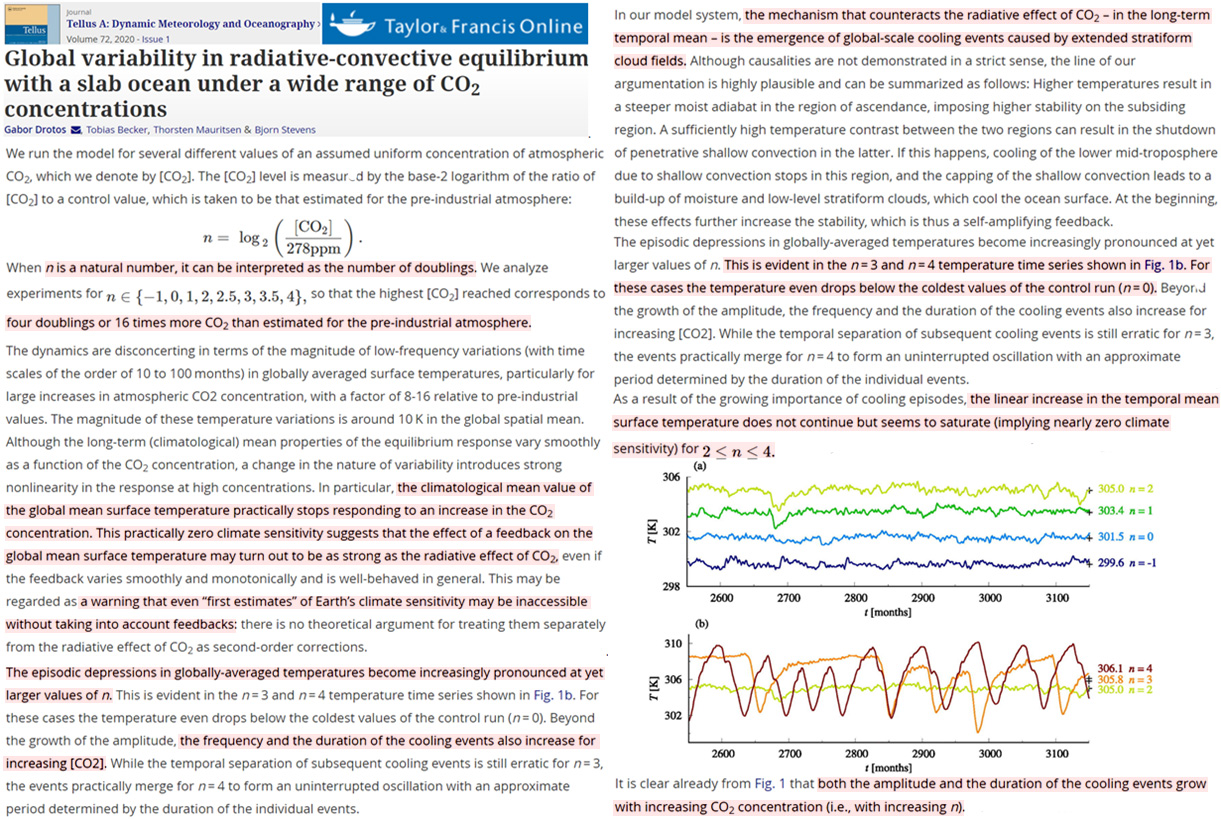
On the contrary the carbon dioxide molecule is not a light polar molecule and has essentially 4 absorption bands in infrared (IR):1.80 micron, 2.0 microns, 4.3 microns, 15 microns [4] The total effect of absorption is essentially due to the water vapor in particular in the visible, infrared, far infrared and very far infrared. On Fig. 1, we can see that water vapor has 10 absorption bands (0.55-0.70 micron) in visible. So, a very great energy is taken by the water directly from the sun in air. Ozone has some absorption. So during the sunny day, it appears that the sun activate the water essentially in our atmosphere. From data [3-6] it is easy to calculate in considering the total absorption areas that the energetic effect ratio between water vapor and CO2 is at least 10. Taking account into the concentrations between water and CO2 in atmosphere is from 10 to 100 following the regions (desert, poles, equator), we deduce that the total energy ratio between water and carbon dioxide for the atmosphere is between 100 (dry air) and 1000 (humid air). … So, it appears the great complexity of the climate: variation of parameters on the Earth (humidity, clouds..), but so the cycles of the sun (11, 22, 60 years…), inclination of Earth axis [13]. Today some authors begin to critic so the theories of GIEC or IPCC [14-16] on the climatic models and even the greenhouse effect saying that is impossible for the atmosphere to heat the Earth because it is cooler.
It is of interest to compare the energetic balance of the Earth with that as a result of human activity. The contemporary released power as a result of human activity is about 2 × 10¹³ W or to the average energy flux of 0.04 W/m2 that is approximately four orders of magnitude below the solar energy flux penetrating in the Earth’s atmosphere. … Let us define the Equilibrium Climate Sensivity (ECS), that is, the change of the global temperature as a result of the doubling of the concentration of CO2 molecules[90]. This quantity may be used as a characteristic of the influence of the atmospheric composition on the global temperature. On the basis of data of Table 6.1, one can obtain for this value [29] ECS = (0.6 ± 0.3) °C.
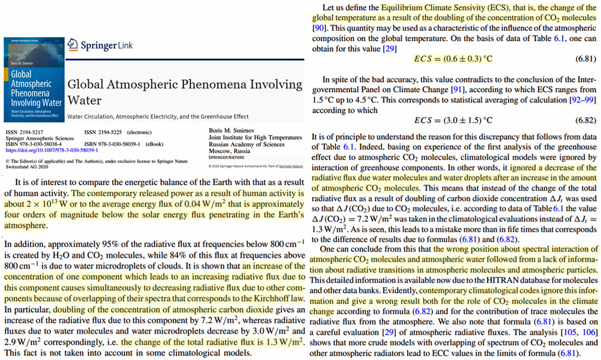
When compared to the average annual global temperature record from 1880, no published climate model posited on the assumption that the increasing concentration of atmospheric carbon dioxide is the driver of climate change can accurately replicate the significant variability in the annual temperature record. Therefore, new principles of atmospheric physics are developed for determining changes in the average annual global temperature based on changes in the average atmospheric concentration of water vapor. These new principles prove that: 1) Changes in average global temperature are not driven by changes in the concentration of carbon dioxide; 2) Instead, autonomous changes in the concentration of water vapor, ∆TPW, drive changes in water vapor heating, thus, the average global temperature, ∆TAvg, in accordance with this principle, Avg ∆ =∆ T 0.4 TPW the average accuracy of which is ±0.14%, when compared to the variable annual, 1880-2019, temperature record
Levendis et al., 2020 (review comments)
Experimental results, plotted in figure 4, showed that upon switching the electric heating element off, its cooling rate was slower in CO2 than in air. For example, in the smallest balloon tested (65 cm), the two cooling curves were separated by a small temperature difference of 0.5 K at 6.5 min, which is at the thermocouple special limit of error. However, in the 75 cm balloon, the temperature difference at 6.5 min increased to a more significant 1.5 K, whereas in the 85 cm balloon, the corresponding temperature difference increased further to 2 K.
[After 6 minutes, 30 seconds, 100% CO2 reduces cooling just ~1.3°C more than 0.05% CO2 does in ambient air.]
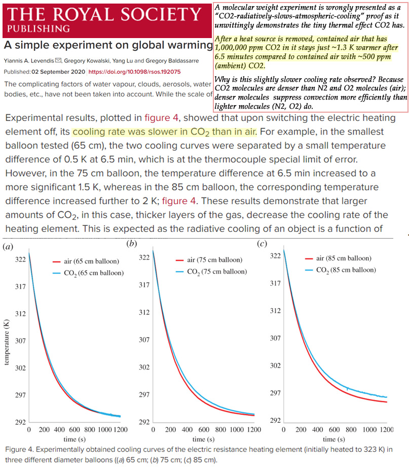
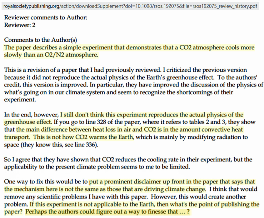
Although it is often noted that greenhouse warming has long been found in the climate literature, it turns out that this was not generally considered a major cause of climate change until the 1980s. … Many factors, including fluctuations of average cloud area and height, snow cover, ocean circulations, etc. commonly cause changes to the radiative budget comparable to that of doubling of CO2. For example, the net global mean cloud radiative effect is of the order of − 20 W/m²cooling effect). A 4 W/m² forcing, from a doubling of CO2, therefore corresponds to only a 20% change in the net cloud effect. … A causal role for CO2 cannot be claimed [for interglacial warming] since its variations (between 180 and 280 ppmv—corresponding to a change in radiative forcing of about 1 W/m²) follow rather than lead the temperature changes. So it is maintained that orbital variations ‘pace’ the glaciation cycles, and that the resulting changes in CO2 provide the necessary ‘amplification’. … Again, the currently widespread explanation takes a different view of this situation. The physics came to be associated exclusively with the greenhouse effect amplified by the alleged positive water vapor feedback. The change in equator-to-pole temperature difference was attributed to some imaginary ‘polar amplification,’ whereby the equator-pole temperature automatically followed the mean temperature [11]. Although the analogy is hardly exact, this is not so different from assuming that flow in a pipe depends on the mean pressure rather than the pressure gradient. … [I]t is implausible that a system as complex as the climate system with mean temperature anomaly) and determined by a single factor (CO2 level in the atmosphere).
[W]e analyzed this correlation and came to the conclusion that it is difficult to explain by the greenhouse effect, which can explain about 500 mK [0.5°C] for a doubling of CO2 in the atmosphere from 350 ppm to 700 ppm; the climate sensitivity of carbon dioxide is d d CO T [ 2 ] = 1.4 mK/ppm [], which we call the open-loop sensitivity (s). It has to be noted that the correlation observed is about 95 mK/ppm [1], two orders of magnitude larger. To circumvent this problem, researchers introduced a positive feedback β in the climate models, such that the overall sensitivity can be any value desired, d d CO 1 , T ss [ 2 ] = − ( β ) including the 95 mK/ppm observed. The parameter β has no justification other than that it can explain the data; it is retrodiction [2]. … We thus expect, on basis of physical laws, to have a climate sensitivity of CO2 smaller than 500 mK [0.5°C] for doubling of CO2 in the atmosphere. This may well be effectively unmeasurable.
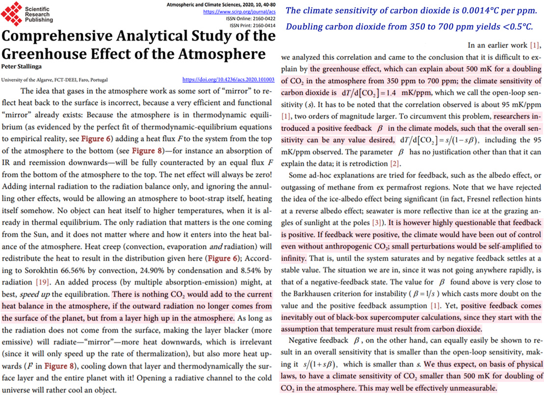
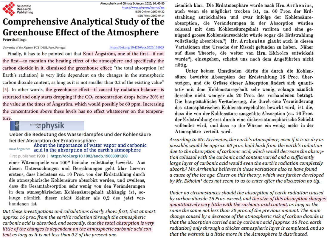
In 2013, and following from 1990, the Intergovernmental Panel on Climate Change (IPCC) issued Climate Change 2013:The Physical Science Basis (AR5) claiming the concentration of CO2, air temperature, and water vapor go up and down together; the air can hold more water vapor and the increased warming by water vapor adds to the warming by CO2. Pictorially: CO2↑, T↑, WV↑. Although no scientific evidence is offered, this concept has become widely accepted because of the fear that CO2 might increase the Earth’s temperature to dangerous levels. In developing research to evaluate the IPCC claims, it is noted that the temperature at the Equator is always higher than that in the Arctic and Antarctic. The Gas Law of Charles/Gay-Lussac states that at constant pressure the volume of a gas is inversely proportional to the absolute temperature. Thus by applying this law, the CO2 concentration is always higher at the Poles than at the Equator. Thus, when moving from the Poles to the Equator, temperature goes up, CO2 goes down and water vapor goes up. Pictorially: T↑, WV↑, CO2↓. The warming effects of CO2 and water vapor do not add; they oppose each other. This is a robust conclusion based on hard numbers. It is opposite to the claim by the IPCC and proves there are errors in the assumptions.
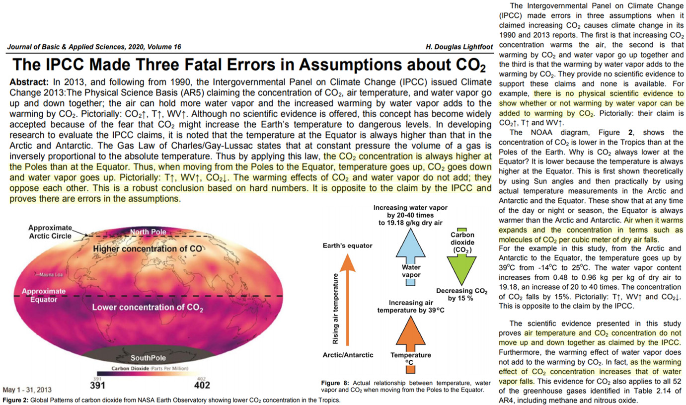
Koutsoyiannis and Kundzewicz, 2020
We examine the relationship of global temperature and atmospheric carbon dioxide concentration at the monthly time step, covering the time interval 1980–2019, in which reliable instrumental measurements are available. While both causality directions exist, the results of our study support the hypothesis that the dominant direction is T → CO2. … For the monthly scale the attained p-values in the direction T → [CO2] are always smaller than in direction [CO2] → T by about 4 to 5 orders of magnitude, thus clearly supporting T → [CO2] as dominant direction. … The results of the study support the hypothesis that both causality directions exist, with T → CO2 being the dominant, despite the fact that the former CO2 → T prevails in public, as well as in scientific, perception. Indeed, our results show that changes in CO2 follow changes in T by about six months on a monthly scale, or about one year on an annual scale. … The change in carbon fluxes due to natural processes is likely to exceed the change due to anthropogenic CO2 emissions, even though the latter are generally regarded as responsible for the imbalance of carbon in the atmosphere. … The opposite causality direction opens a nurturing interpretation question. We attempted to interpret this mechanism by noting that the increase of soil respiration, reflecting the fact that the intensity of biochemical process increases with temperature, leads to increasing natural CO2 emission.
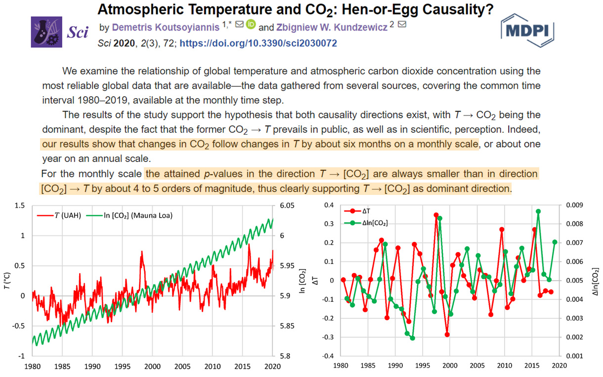
A conclusion of this study is that the calculations carried out by the way as defined by the IPCC do not indicate any positive water feedback mechanism in the atmosphere. There are now together three independent calculation methods resulting in the same conclusion and the humidity versus temperature observations show the same. In practical calculations, amazingly simple equations can be applied in calculating the temperature impacts of RF by using the λ value of 0.27 Wm-2. … Stratospheric cooling can be deducted by the general knowledge of radiation behavior in the stratosphere and the numerical calculations confirm these analyses. The results of this study show that stratospheric cooling happens when CO2 concentration increases but its effect on radiative forcing is negative and not positive as reported in many studies. It means that the concept of ERF being the sum of instantaneous radiative forcing (IRF) plus rapid adjustments can be challenged to have serious flaws. If the stratospheric cooling has a negative effect of RF, then also the IRF magnitude has been wrongly calculated in GCMs.
The contribution to the total radiative flux for the real (standard) atmosphere is 51% due to water molecules, 29% due to water microdroplets (clouds), 18% due to CO2 molecules, and 2% due to CH4 and N2O molecules. In addition, 98% of the flux of infrared radiation at wavelengths below 12.5 µm is created by H2O and CO2 molecules, whereas 85% of the radiative flux at wavelengths above 12.5 µm is due to clouds. If the concentration of atmospheric CO2 molecules is doubled without a change the other atmospheric param-eters, the change of the radiative flux to the Earth due to CO2 molecules is 7.2 W/m2, whereas the change of the total radiative flux with accounting for screening fluxes from other components is 1.3 W/m2 that corresponds to the global temperature change of 0.6 ± 0.3 K. Usually climatological models do not account for the interaction between greenhouse that leads components to a six times larger temperature change. One can compare the latter value with results of NASA programs for the analysis of evolution of the carbon dioxide concentration and the global temperature. From this it follows that doubling of the concentration of atmospheric CO2 molecules is accompanied by the change of the global temperature according to (14). Thus, in the real atmosphere only a forth part of the global temperature change occurs due to variation of the concentration of CO2 molecules results from the greenhouse effect involving these molecules.
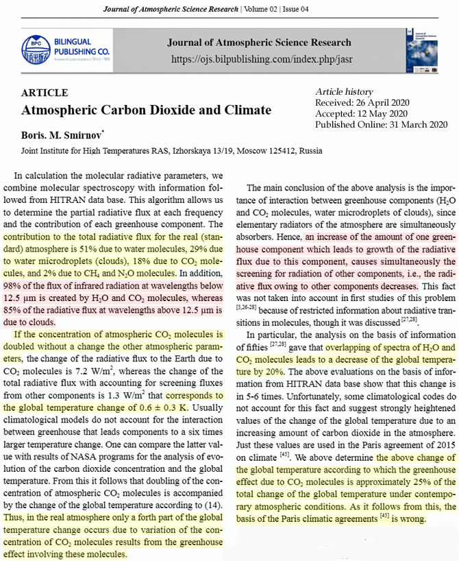
Unsettled Science, Failed Climate Modeling
Cloud plays important roles in the climate system through the radiation processes and hydrological cycle of the Earth (Trenberth et al., 2009). Therefore, cloud must be simulated appropriately in general circulation models (GCMs) for climate change assessments. However, despite its important roles in the climate system, cloud has not been simulated accurately, and it remains one of the greatest factors of uncertainty in climate predictions, as reported by the Fifth Intergovernmental Panel on Climate Change (IPCC AR5: Stocker et al., 2013). This has prompted a number of scientific efforts to reduce uncertainties in climate predictions due to cloud. …. the observation error SDs for OSR and OLR were estimated to be 0.14 and 33.1 (W/m²), respectively. Although the error estimates for the satellite products are not available, these values are similar to globally averaged SDs of natural variability for OSR and OLR in the diagnosed period (0.10 and 24.9 W/m²).
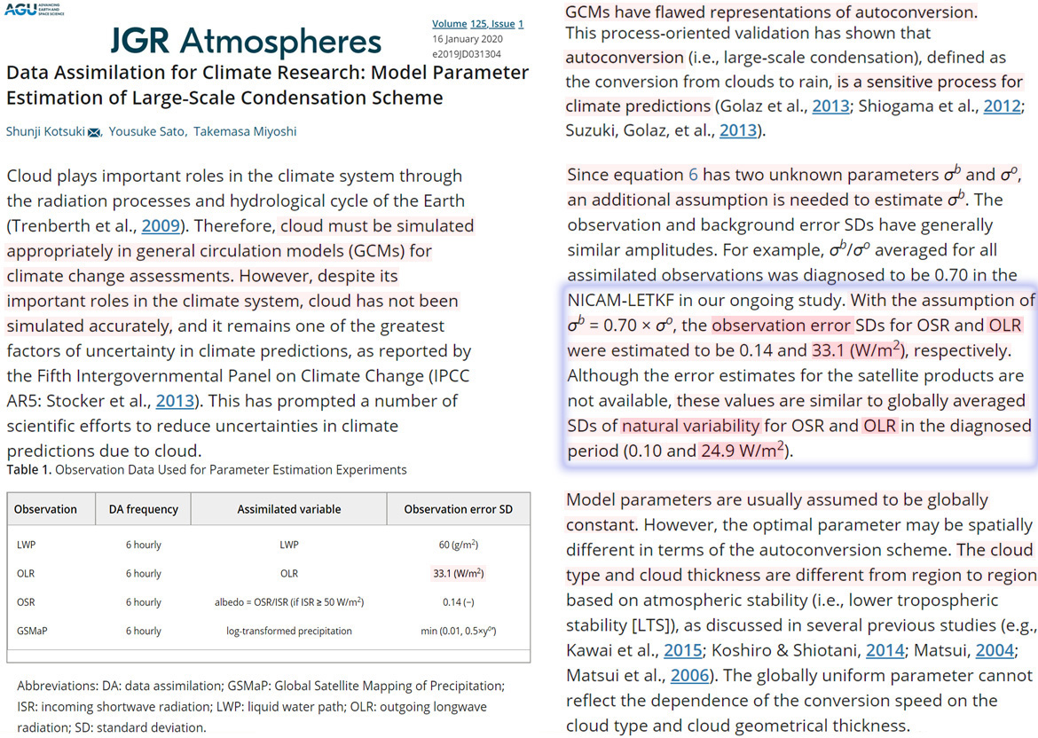
Stratocumulus cloud‐top entrainment has a significant effect on cloud properties, but there are few observations quantifying its impact. Using explicit 0D parcel model simulations, initialized with below‐cloud in‐situ measurements, and validated with in‐situ measurements of cloud properties, the shortwave cloud radiative forcing (SWCF) was reduced by up to 100 W m‐2 by cloud‐top entrainment in the Southern Ocean. The impact of entrainment‐corrected SWCF is between 2 and 20 times that of changes in the aerosol particle concentration or updraft at cloud base. The variability in entrainment‐corrected SWCF accounts for up to 50 W m‐2 uncertainty in estimating cloud forcing.
The resulting regional uncertainties in clear-sky surface downward fluxes are 6 W m−2 for SW and 8 W m−2 for LW (Table 5). In the LW, the uncertainties for all sky and clear sky are comparable, but for SW the all-sky uncertainty is over a factor of 2 larger than clear sky. For the regional uncertainty in the clear-sky upward SW and LW fluxes, we assume that the uncertainty is the same as the all-sky uncertainty because the uncertainty in surface albedo, emissivity, and surface skin temperature are largely contributing the upward flux uncertainty. … Regional uncertainties in surface net flux, SW + LW flux, and CRE are determined by accounting for the upward and downward flux uncertainties and their covariance. We compute the latter using surface flux adjustments applied to computed fluxes when CERES-derived TOA fluxes are used to constrain surface fluxes. In the process, surface, atmosphere, cloud, and aerosol properties are adjusted to match computed TOA fluxes with TOA fluxes derived from CERES observations (Kato et al. 2018). Based on the adjustment of these properties, surface SW and LW upward and downward fluxes are also adjusted. Therefore, surface flux adjustments are considered to be the error in the surface fluxes due to errors in inputs used in the computation. Temporal error correlations are derived from regional surface flux adjustments averaged over the entire globe using the time period from March 2000 through February 2016. Regional uncertainties are 18 W m−2 for LW net downward flux, 16 W m−2 for SW net downward flux, and 26 W m−2 for SW + LW Net
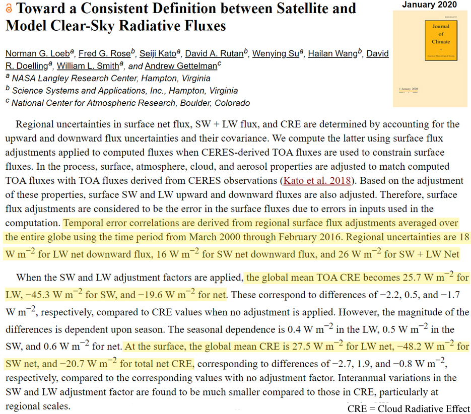
In particular, most climate models that participated in the Coupled Model Intercomparison Project Phase 5 (CMIP5) were found to have too little shortwave radiation being reflected back to space and excessive shortwave radiation reaching the surface over the Southern Ocean – an error with significant consequences for predicting both regional and global climate. … [M]ost CMIP5 models have a negative longwave (LW) bias due to insufficient longwave cloud radiative forcing. On average, the water masses of the Southern Ocean in the CMIP5 models are too warm and light, also likely due in part to excess heat uptake (Sallée et al. 2013). These model radiative errors and associated excess heat uptake are of profound importance to global climate
Clouds are poorly represented in climate models. This has been attributed to factors that include simulating too little cloud cover and under-representing the amount of supercooled liquid water in clouds. This leads to biases the cloud radiative effect, which in turn causes a positive shortwave radiation bias over the Southern Ocean, where too much sunlight is hitting the surface of the ocean.
The Clouds and the Earth’s Radiant Energy System (CERES) Energy Balanced and Filled (EBAF) Edition 4.1 data product provides global surface irradiances. Uncertainties in the global and regional monthly and annual mean all-sky net shortwave, longwave, and shortwave plus longwave (total) irradiances are estimated using ground-based observations. Error covariance is derived from surface irradiance sensitivity to surface, atmospheric, cloud and aerosol property perturbations. Uncertainties in global annual mean net shortwave, longwave, and total irradiances at the surface are, respectively, 5.7 Wm−2, 6.7 Wm−2, and 9.7 Wm−2. In addition, the uncertainty in surface downward irradiance monthly anomalies and their trends are estimated based on the difference derived from EBAF surface irradiances and observations. The uncertainty in the decadal trend suggests that when differences of decadal global mean downward shortwave and longwave irradiances are, respectively, greater than 0.45 Wm−2 and 0.52 Wm−2, the difference is larger than 1σ uncertainties.
The accuracy of SCOPE is evaluated using one year (2018) of downwelling longwave (DLW) radiation measurements from the Surface Radiation Budget Network, which consists of seven sites spread across climatically diverse regions of the contiguous United States. During daytime clear-sky periods, SCOPE predicts DLW within instrument uncertainty (10 W m−2) for four of the seven locations, with the remaining locations yielding errors of the order of 11.2, 17.7, and 20.2 W m−2. For daytime cloudy-sky, daytime all-sky (clear or cloudy), and nighttime all-sky periods, SCOPE achieves root mean square error values of 23.0–34.5 W m−2 for all seven locations.
All model runs warmed faster than observations in the lower troposphere and midtroposphere, in the tropics, and globally. On average, and in most individual cases, the trend difference is significant. … [W]e present evidence that the distribution of ECS values across the model is unrealistically high.
Very intriguing is however, that 7 out of 13 models show positive ΔR [cloud feedbacks] in the Arctic while the other 6 have negative values. This implies that half of the models analyzed here simulate local runaway climate systems in which the gain of energy is larger than the loss of energy if advection is not taken into account. These models increase the initial radiative perturbation rather than to reduce it. On the other hand, models exhibiting little warmings tend to be dominated by the negative Planck feedback and can be brought back to radiative balance without the contribution of advection.
In spite of the unabated emissions of greenhouse gases into the atmosphere, sea ice around Antarctica has increased over most of the satellite era. Such an increase is not captured by climate models, which simulate a melting over the same period. Over the last few years, moreover, the observed sea ice trends have drastically changed, and this might act to cancel the models‐observations discrepancy. Here we show that in spite of the very recent Antarctic sea ice trend changes, such discrepancy still exists. Analyzing multiple large ensembles of model simulations, we elucidate the origin of the models‐observations discrepancy. We show that internal variability cannot account for the discrepancy, which therefore is likely to stem from biases in the models’ forced response to the external forcing. These biases, we show, reside in thermodynamic ocean‐atmosphere coupling, as models fail to simulate the trends in surface heat fluxes from reanalyses over the period 1979–2019.
The uncertainty of the outgoing longwave fux at the TOA as measured by CERES due to the uncertainty in calibration is ~ 3.7 W m−2 (2 σ), whereas the uncertainty in the shortwave refected fux is ~ 2% (2 σ), or equivalently 2 Wm−2 (Loeb et al. 2009). … But note also the large spread in the global mean downward shortwave radiation at the Earth’s surface amongst the various CMIP6 models in Fig. 3 (upper panel), which amounts to as much as 21 Wm−2. This spread is more than 8 Wm−2 larger than the spread in the corresponding surface absorbed shortwave radiation (Table 1). … Indeed the inter-model spread amongst the magnitudes of the global energy balance components in the individual CMIP6 models is still unsatisfactorily large, typically on the order of 10–20 Wm−2. The substantial inter-model spread of 18 Wm−2 in the simulated global mean surface latent heat fux further points to considerable discrepancies not only in the representation of the global energy cycle, but also of the global water cycle in the CMIP6 models. All these discrepancies have generally not decreased from the previous model generation CMIP5 to the latest model generation CMIP6, and the inter-model spreads and standard deviations remain similar. Thus, there is no clear sign of convergence in the energy budget estimates of current state-of the art climate models.
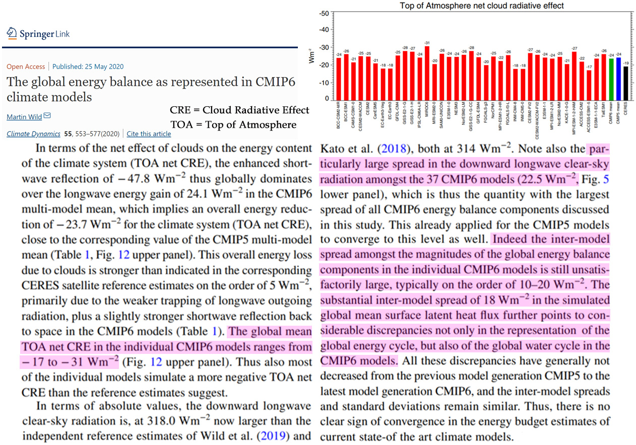
The four datasets capture a large fraction (> 40%) of the interannual variability in the ice core snow accumulation composite over the Antarctic Peninsula from 1901 to 2010. However, none of the twentieth century datasets alone is able to explain > 20% of variance in ice core records at the other Antarctic regions during the twentieth century. Even for the modern satellite era (from 1979 onwards), their performance for Antarctic snow accumulation is still poorer, relative to ERA-Interim, RACMO2 and MAR. Considerable inhomogeneities and spurious changes in atmospheric circulation are found in these datasets, and thus the precipitation minus evaporation/sublimation (P–E) changes and trends during the past 100 years are largely artificial over Antarctica.
Their prediction of global C[arbon] export from the Ez [euphotic zone, the section of upper ocean layer that sunlight is able to penetrate] is 5.7 Pg C⋅y−1, with large regional variability, including higher Ez-ratios at high latitudes, a finding consistent with this compilation here. If their same model with a fixed b and export depth of 150 m is used, global fluxes decrease by twofold (2.8 Pg C⋅y−1) and the regional gradients in Ez-ratio largely disappear. Given that much of the world’s oceans have shallow Ezs, any assessment that does not consider an Ez-normalized framework will always produce lower average POC fluxes and export ratios, particularly at higher latitudes. … Importantly for C[arbon] sequestration and climate, the impact on global carbon budgets is also large, with export being a factor of 2 higher for an Ez-normalized C flux, compared with using the canonical fixed 150-m depth flux assessment.
The world’s oceans play an important role in regulating the amount of carbon dioxide in the atmosphere by absorbing billions of metric tons of it each year. A new study suggests we may have been greatly underestimating the effectiveness of this vast carbon sink, with new modeling from scientists at Woods Hole Oceanographic Institution (WHOI) finding that the ocean’s “biological pump” is actually capturing twice as much CO2 as previously thought. … Instead of relying on measurements taken at fixed depths, the scientists instead used data gathered from chlorophyll sensors, which reveal the presence of the phytoplankton and therefore the true edges of the euphotic zone. Following this analysis, the team concluded that the depths of this boundary vary around the world, and taking this into account the ocean absorbs around twice as much carbon each year than we had thought.
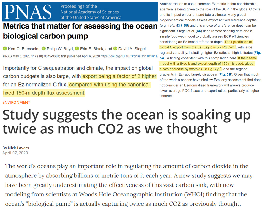
Iliopoulou and Koutsoyiannis, 2020
A relevant case study by Lee and Ouarda (2010) concluded that predictions of decadal streamflow extremes using the NAO as a covariate were impacted by large uncertainty to the point of almost being non-informative. … From a systematic investigation of long-term rainfall records, corroborated by simulation results, we have verified that local trends have poor out-of-sample performance, being outperformed in their predictions by simpler models, as the local mean. This empirical finding suggests that the large inherent variability present in the rainfall process makes the practice of extrapolating local features in the long-term future dubious, especially when the complexity of the latter increases. This in turn questions the theoretical and practical relevance of projections of rainfall trends and the grounds of the related abundant publications. … The entire question however relies on a simplistic view of complex systems, i.e. that just one factor (or the change thereof) suffices to determine the system’s future evolution. In our view, this is not a logically consistent framework for dealing with complex systems.
[D]ynamical changes in atmospheric circulation are very uncertain. This leads to low confidence in regional projections, especially for precipitation, over the coming decades. The chaotic nature of the climate system may also mean that signal uncertainties are largely irreducible. However, climate projections are difficult to verify until further observations become available. Here we assess retrospective climate model predictions of the past six decades and show that decadal variations in North Atlantic winter climate are highly predictable, despite a lack of agreement between individual model simulations and the poor predictive ability of raw model outputs. Crucially, current models underestimate the predictable signal (the predictable fraction of the total variability) of the North Atlantic Oscillation (the leading mode of variability in North Atlantic atmospheric circulation) by an order of magnitude. Consequently, compared to perfect models, 100 times as many ensemble members are needed in current models to extract this signal, and its effects on the climate are underestimated relative to other factors.
The study, which includes authors from several leading modeling centers, casts doubt on many forecasts of regional climate change, which are crucial for policymaking. It also means efforts to attribute specific weather events to global warming, now much in vogue, are rife with errors. “The whole thing is concerning,” says Isla Simpson, an atmospheric dynamicist and modeler at the National Center for Atmospheric Research, who was not involved in the study. “It could mean we’re not getting future climate projections right.” Kirtman thinks something fundamental is wrong with the models’ code. For the time being, he says, “You’re probably making pretty profound mistakes in your climate change assessment” by relying on regional forecasts. For example, models predicted that the Horn of Africa, which is heavily influenced by Indian Ocean winds, would get wetter with climate change. But since the early 1990s, rains have plummeted and the region has dried. The missing predictability also undermines so-called event attribution, which attempts to link extreme weather to climate change by using models to predict how sea surface warming is altering wind patterns. The changes in winds, in turn, affect the odds of extreme weather events, like hurricanes or floods. But the new work suggests “the probabilities they derive will probably not be correct,” Smith says.
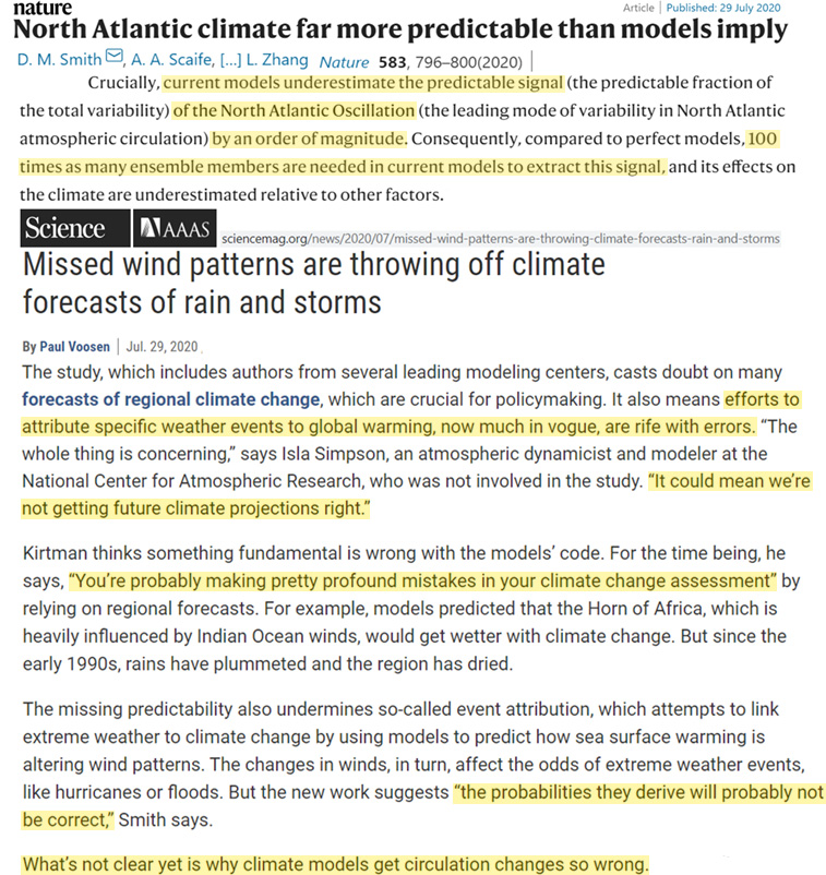
In the atmosphere, microphysics ‐ the small‐scale processes affecting cloud and precipitation particles such as their growth by condensation, evaporation and melting ‐ is a critical part of Earth’s weather and climate. Because it is impossible to simulate every cloud particle individually owing to their sheer number within even a small cloud, atmospheric models have to represent the evolution of particle populations statistically. There are critical gaps in knowledge of the microphysical processes that act on particles, especially for atmospheric ice particles because of their wide variety and intricacy of their shapes. The difficulty of representing cloud and precipitation particle populations and knowledge gaps in cloud processes both introduce important uncertainties into models that translate into uncertainty in weather forecasts and climate simulations, including climate change assessments. … [T]he sheer number of particles is simply too large to model explicitly every hydrometeor within a cloud, even with massive advances in computing power. Even in a fairly small cloud with a volume of 1 km3, the total number of particles can easily exceed 1017. Thus, particle-by-particle DNS will remain confined to domains much smaller than most individual clouds, and the hydrometeor population will need to be parameterized in almost all models into the foreseeable future. Second, and perhaps even more troubling: even at the scale of individual cloud and precipitation particles, many microphysical processes are poorly understood. This is notably different from other subgrid-scale components of atmospheric models, such as turbulence and radiation, for which complete governing equations or benchmark models are available, e.g., the Navier-Stokes equations for turbulence and line-by-line models for radiation. Moreover, there is no well-defined physical scale at which microphysical processes are fully “resolved” … In practice, the most sophisticated microphysics scheme in any atmospheric model, even in particle-by-particle DNS, can only attempt to represent a small subset of these processes. … Although hydrometeor fluxes can be directly obtained in-situ from disdrometer and remotely from Doppler radar and lidar, we emphasize the general difficulty of quantifying rates for individual microphysical processes directly from cloud and precipitation observations in natural clouds; multiple processes are often active under uncontrolled conditions and measurements needed to obtain these rates are usually incomplete. Even in the controlled setting of a laboratory, what can be measured is often different from what is needed by schemes, and sometimes the fundamental measurement itself is not yet possible. This means it has been difficult or even impossible to constrain many individual process rates in schemes directly from observations. … [O]ne of our central arguments is that microphysics scheme complexity is “running ahead” of current cloud physics knowledge and the ability to constrain schemes observationally. Fundamentally, this calls into question not only the realism of these schemes at their core, but whether or not in principle they are even verifiable in any kind of rigorous way. This presents a troubling picture moving forward. … Quoting from Sir Karl Popper, preeminent philosopher of science in the 20th century [Popper, 1959]: “In so far as a scientific statement speaks about reality, it must be falsifiable: and in so far as it is not falsifiable, it does not speak about reality” (this generalizes a well-known statement from Einstein [1921]). Furthermore, while it is clear that schemes are largely uncertain, the degree to which they are uncertain remains mostly unquantified. Indeed, the design of most schemes has made it very difficult to quantify uncertainty systematically. This has been a critical limitation.
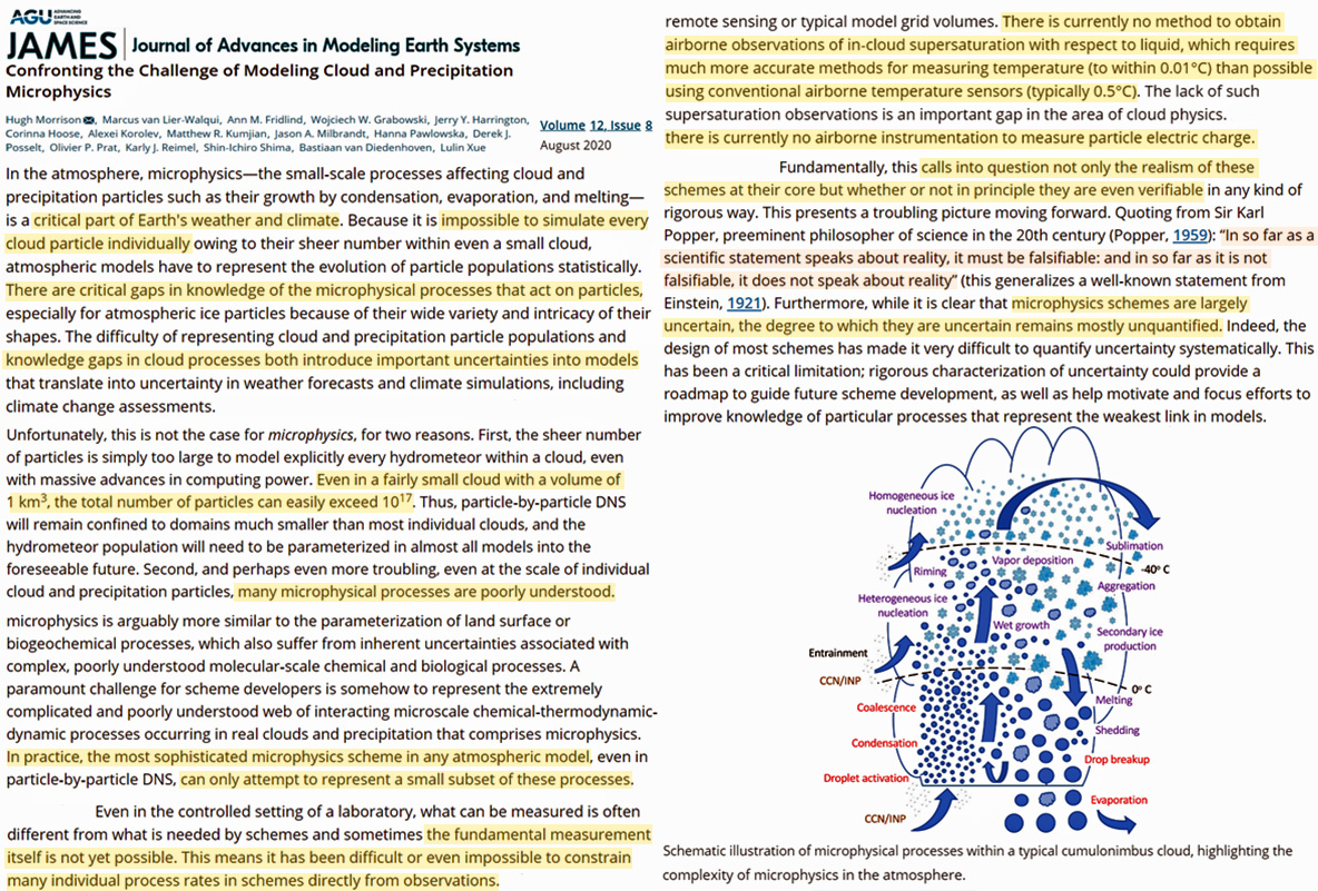

The differences in downward longwave radiation can reach −60 W/m2 in valleys without considering terrain effects. Based on the reference of hemispherical upward longwave radiation, surface upward longwave radiation estimated by the direct estimation method had a bias of 11.41 W/m2 and standard deviation (STD) of 7.30 W/m2, while the directional upward longwave radiation had a bias of 5.99 W/m2 and STD of 4.08 W/m2, showing lower estimation variation. The discrepancy between surface net longwave radiation (NLR) and terrain-corrected NLR ranged between 50 and −130 W/m2 with clear negative biases mainly occurring in valleys. With higher spatial resolutions of remotely sensed imagery, the influence of complex terrain on land surface radiative flux has become more significant.
Hydrological trends not following modeled expectations
The analyses of atmospheric water, as well as those of precipitation and evaporation, reveal two important points: (a) all processes fluctuate in time at all time scales and (b) no monotonic trends that would be attributed to temperature increase appear in any type of data. In some cases (e.g. satellite observations of water vapour amount) there appear some trends, which, however, are opposite to established expectations. … As a result of intensification of disaster reporting, people think that rainfall events have become more intense or frequent recently. However, based on a list of world record point precipitation measurements compiled by Koutsoyiannis and Papalexiou (2017) for various time scales ranging from 1 min to 2 years, the fact is that the highest frequency of record rainfall events occurred in the period 1960-80; later the frequency was decreased remarkably. … A more detailed analysis can be based on the four sources of daily rainfall information analysed here. This analysis has been performed separately for each continent and its results are presented graphically. Figure 17 shows the temporal evolution of the monthly maximum daily precipitation areally averaged over the continents. Figure 18 shows similar information but for the areally maximum, over each continent, monthly maximum daily precipitation. None of the figures in none of the continents and none of the sources of data provides support on the intensification allegation. In particular, the observational data (CPC and GPCP) could support the opposite hypothesis, that of extreme rainfall deintensification. This becomes even more evident if we examine the temporal evolution of standard deviation of daily precipitation in each month, averaged over land. In this respect, Figure 19, shows that deintensification, expressed as decreasing standard deviation, is evident in the 21st century both from CPC and GPCP observational data. The same is shown in a different manner in Figure 20 in terms of precipitation rate exceeding a threshold. Clearly, neither the frequency of high precipitation nor the sum of high intensity precipitation is intensifying. Rather, in most of the cases, there has been deintensification in the 21st century. … In fact, the established climatic hypotheses on hydrological cycle are not validated by the data analysed. Relative humidity is decreasing in the entire atmosphere, instead of being constant. Specific humidity is increasing at a rate of about 1/3 of that implied by established hypotheses. Water vapour amount is fluctuating without a monotonic trend. Precipitation and evaporation again fluctuate. The precipitation extremes and their frequencies also fluctuate. Fluctuations are successions of intensification and deintensification, with deintensification prevailing in the 21st century.
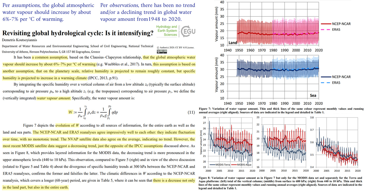
We propose that the vapor buoyancy effect can increase Earth’s OLR and helps stabilize Earth’s climate by regulating the atmosphere’s thermal structure. Figure 1 shows the temperature and virtual temperature (buoyancy) fields in the moisture space from 2°S to 2°N using NASA AIRS data. In the free troposphere (p < 850 hPa), buoyancy is horizontally uniform because of the small Cori olis parameter and efficient gravity waves (Charney 1963; Bretherton and Smolarkiewicz 1989; Sobel et al. 2001; Yang 2018a). However, temperature increases toward dry columns due to the vapor buoyancy effect. Moving toward the dry columns, moisture and its associated vapor buoyancy are reduced. To maintain uniform buoyancy, temperature has to increase. … Although there is no such constraints in the boundary layer, we can assume that ∆T = 0 at the surface temperature because of the uniform sea surface temperature (SST). We, therefore, require ∆T equals ∆TW BG in the free troposphere but smoothly decays to 0 at surface: ease with climate warming due to increasing atmospheric moisture, leading to enhanced OLR over the dry area. This is a negative feedback which can help to stabilize Earth’s climate.
The effect of irrigation on temperature has attracted much attention because its cooling effect may mask the warming due to other factors, such as greenhouse gas forcing. Although many studies have examined the irrigation cooling effect (ICE) based on near-surface air temperature from meteorological observations or climate model simulations, few studies have directly addressed the effect of irrigation on land surface temperature (LST), which is closely linked to the surface energy balance and near-surface air temperature. In this paper, an ICE detection (ICED) method is proposed to assess the effect of irrigation on LST using the Moderate Resolution Imaging Spectroradiometer (MODIS) products across China. The magnitude of the ICE is calculated as the LST difference between irrigated area and adjacent non-irrigated area in the self-adaptive moving window determined by the ICED method. The results show that irrigation cools daytime LST by 1.15 K, and cools nighttime LST by 0.13 K, on average, across irrigated areas in China. The effect of irrigation on LST differs greatly among the climate zones and seasons, characterized by the enhanced ICE in arid regions and the growing season. In the arid climate zone, nearly all the irrigated areas show a lower daytime LST than the adjacent non-irrigated areas, leading to a strong ICE magnitude of >6 K in the growing season.
Contrary to expectations that global warming will be accompanied by an increase in terrestrial evaporation, pan evaporation (PE) has decreased in several parts of the world during the last decades.
Failing Renewable Energy, Climate Policies
A commonly held idea is that substituting wood for fossil fuels or energy intensive materials reduces greenhouse gas (GHG) emissions. … When comparing wood fuel to fossil fuels as regards climatic impacts, the pertinent physical characteristic is the CO2 emission factor, that is the amount of carbon (or carbon dioxide) emitted per unit of released energy. Values of this intrinsic emission factor taken from a standard source are shown in Table 1 (second column) for representative fuels. The combustion emission of wood is clearly higher than that of other fuels. … Just after combustion, displacement factors exhibit negative values, whatever the displaced fossil fuel39, as shown in the fourth column of Table 1. As the wood carbon footprint is increased transiently by a value in the order of the carbon content Qr(0) of the residues (extremum), the apparent wood emission factor is itself increased, reaching a peak up to 170 kgCO2eq/ GJ or thereabouts if all crop residues are left in place. This estimate gives support to the rough affirmation that the carbon emission from wood fuel is bigger by half than that from coal, twice that from oil and three times that from gas, for the same energy released.
After a first rotation of harvesting, carbon stocks declined 33–50% relative to stocks in the natural, fire-dominated landscapes and payback periods ranged from 92 to 757 years. The type of fossil fuel had the strongest effect on payback periods: under average efficiencies, ranges were 122–207, 156–268 and 278–481 years for coal, oil and natural gas respectively. These calculations suggest that under a wide range of assumptions, clearcut-based management of boreal primary landscapes to produce wood pellets to replace fossil fuels in electricity generation will result in net emissions of greenhouse gases to the atmosphere for many decades. … In conclusion, our calculations indicate that clearcut harvesting of boreal primary forests to replace fossil fuel use in electricity generation entails considerable carbon debt payback periods, which are in the range of 122–481 years for mid-range conversion efficiencies. Debts increased as the mismatch between natural fire intervals and rotation periods increased. More generally, we argue that the magnitude of such debts makes it unlikely that clearcut logging of primary forests can serve as a climate change mitigation strategy and that mitigation would be better served by increased conservation of primary forests and use of harvesting methods that entail lower offtakes over longer periods of time.
We find that studies projecting a large role of forest bioenergy in climate change mitigation rely on assumptions that are too optimistic, at times outright unrealistic.
Wind Power Harming The Environment, Biosphere
The global wind energy council (GWEC) has predicted a 17-fold increase in generaton of wind energy by 2030 (Lu et al. 2009). Such expansion in wind energy producton poses serious threats to flying vertebrates (Peron et al. 2013; Singh et al. 2015). This study reveals that 12 local and three migratory species of birds in Bakkhali are vulnerable to collision with wind turbines. There is utmost urgency to modify design of wind turbines to save these birds from collision. Further studies are required to assess accurate causes of bird fatalites near wind farms in India, detailed assessment of the most affected local and migratory species of birds, their dependency with other species, and implementaton of additonal & complementary measures to protect birds from wind turbines. As a future extension, one needs to conduct risk analysis through robust statstcal analysis.
Bird and bat fatalities increase with wind energy expansion and the only effective fatality‐ reduction measure has been operational curtailment, which has been documented for bats but not for birds. We performed opportune before‐after, control‐impact (BACI) experiments of curtailment effects on bird and bat fatalities and nocturnal passage rates during fall migration at 2 wind projects, where 1 continued operating and the other shut down from peak migration to the study’s end (study 1). … Of bird species represented by fatalities in study 2, 79% were found at inoperable wind turbines. Because the migration season is relatively brief, seasonal curtailment would greatly reduce bat fatalities for a slight loss in annual energy generation, but it might not benefit many bird species.
Wind energy production has expanded to meet climate change mitigation goals, but negative impacts of wind turbines have been reported on wildlife. Soaring birds are among the most affected groups with alarming fatality rates by collision with wind turbines and an escalating occupation of their migratory corridors. These birds have been described as changing their flight trajectories to avoid wind turbines, but this behaviour may lead to functional habitat loss, as suitable soaring areas in the proximity of wind turbines will likely be underused. We found that areas up to approximately 674 m away from the turbines were less used than expected given their uplift potential. Within that distance threshold, bird use decreased with the proximity to wind turbines. We estimated that the footprint of wind turbines affected 3%–14% of the areas suitable for soaring in our study area. … We present evidence that the impacts of wind energy industry on soaring birds are greater than previously acknowledged. In addition to the commonly reported fatalities, the avoidance of turbines by soaring birds causes habitat losses in their movement corridors.
Our rates of observed bat collisions, adjusted for the rates of unseen collisions, would predict four to seven times the fresh fatalities we found using dogs between two wind projects. Despite markedly improved carcass detection through use of dogs, best estimates of bat fatalities might still be biased low due to crippling bias and search radius bias. … With the near doubling of installed wind energy capacity to 100,125 MW by September 2019, and if annual bat fatalities are proportional to installed capacity and the number of bats vulnerable to collision undiminished, then extrapolating from a 2012 estimate [3] would predict >1.7 million bat fatalities in the USA in 2019 (95% CI: 746,207–2,699,370). If we restrict mean fatality rates to those estimated from fatality search intervals < 10 days, which increased bat fatality estimates over the overall mean fatality rate, then estimated annual fatalities in 2019 would have increased to 3,719,043 bats (95% CI: 1,770,510 to 5,667,676).
[R]enewable energy facilities can be landuse intensive and impact conservation areas, and little attention has been given to whether the aggregated effect of energy transitions poses a substantial threat to global biodiversity. Here, we assess the extent of current and likely future renewable energy infrastructure associated with onshore wind, hydropower and solar photovoltaic generation, within three important conservation areas: protected areas (PAs), Key Biodiversity Areas (KBAs) and Earth’s remaining wilderness. We identified 2,206 fully operational renewable energy facilities within the boundaries of these conservation areas, with another 922 facilities under development. Combined, these facilities span and are degrading 886 PAs, 749 KBAs and 40 distinct wilderness areas. … Our results show that renewable energy development has already encroached on many of the world’s most important places for conserving biodiversity, with 2,206 facilities already operational within PAs [protected areas], KBAs [key biodiversity areas] and wilderness areas (Figure S2). Furthermore, the number of active renewable energy facilities inside important conservation areas could increase by ~42% by 2028, suggesting conflicts will likely intensify in the near future. … This is especially worrying, when assessments show the growth required to achieve the UN climate targets by 2060 (Bauer et al., 2017; IEA, 2017b) would be an order of magnitude greater than the installed capacity included in our ‘operational’ and ‘under development’ datasets. … Our results also show that the spatial distribution of overlaps is moving from developed regions towards more biodiverse developing regions such as Southeast Asia and sub-Saharan Africa, where the consequences for global biodiversity conservation will be more intense.
Oceanic Biosphere Thrive In Warm, High CO2 Environments
We investigated submarine groundwater discharge (SGD) in a volcanic coastal area that hosts the world’s most biodiverse reefs. Measurements of 222Rn activity in coastal seawater, a tracer for groundwater, indicated prevalent SGD. In areas where seawater 222Rn activity was generally higher, we discovered hydrothermal springs emitting acidic waters (pH ~5.4–6.0) and venting magmatic CO2 that brought local pCO2 levels up to 95,000 ppm. The collection of vents raised CO2 and lowered pH over 1–2 km of coastline. … Taking the CO2 sensor to the discharge points revealed what are likely the highest local pCO2 values measured in coastal waters. The most dramatic levels were found in an area with relatively deep bubble vents. This area, hereafter named Soda Springs, is at a water depth of 55 m and is within Secret Bay (Fig. 2D and Supplementary Movies S1 and S2). pCO2 ranged from 60,000-95,000 ppm right at Soda Springs. A few tens of meters away from Soda Springs and towards shore is a broad sandy area at a depth of 50 m with curtains of bubble streamers (Fig. 2E and Supplementary Movies S1 and S2). The pCO2 at this site ranged from 4,000-6,000 ppm (Fig. 2E). The pH of a water sample collected at this site was 6.65. … The SHV springs emit acidic thermal waters with a measured pH range of 5.42-6.85, which is much lower compared to open seawater with a pH of 8.11 measured hundreds of meters offshore. In-situ temperatures measured with conductivity-temperature-depth (CTD) probes range from 50-55°C at the point of discharge. Discrete samples of the coastal seawater within a few tens of meters off the coast and where SHVs are present have a pH of 6.50-7.90. … The submarine spring waters also contribute dissolved CO2 to the coast. Spring waters were analyzed for pCO2 using the same sensor that was used for the in-situ measurements. The submarine spring waters from Bubbles, the source of samples J and K in Fig. 3, had a pCO2 of 29,550 and 38,364 ppm, respectively. Porewater samples collected from the seabed at Bubbles had even higher pCO2 levels of 76,876 and 78,679 ppm. Water from a beach spring (sample B) and water from a deep domestic well at the Planet Dive Resort had a pCO2 of 8,767 and 8,842 ppm, respectively.
Diving 200 feet under the ocean surface to conduct scientific research can lead to some interesting places. For University of Texas at Austin Professor Bayani Cardenas, it placed him in the middle of a champagne-like environment of bubbling carbon dioxide with off-the-chart readings of the greenhouse gas. … The scientists measured CO2 concentrations as high as 95,000 parts per million (ppm), more than 200 times the concentration of CO2 found in the atmosphere. The readings range from 60,000 to 95,000 and are potentially the highest ever recorded in nature. … “These high CO2 environments that are actually close to thriving reefs, how does it work?” said Cardenas, who is a professor in the Jackson School of Geosciences at UT Austin. “Life is still thriving there, but perhaps not the kind that we are used to. They need to be studied.”
Herein, we have characterized an area of volcanic acidification at Mayreau Island, St. Vincent and the Grenadines. Despite localized CO2 enrichment and gas venting, the surrounding area has high hard and soft coral cover, as well as extensive carbonate frameworks. Twice daily extremes in acidification [with pH levels as low as 6.540], in some cases leading to undersaturation of aragonite, are correlated with tidal fluctuations and are likely related to water flow. Corals persisting despite this periodic acidification can provide insights into mechanisms of resilience and the importance of natural pH variability on coral reefs. … To date, natural acidification hotspots have been identified corresponding to upwelling (Manzello 2010), submarine groundwater discharge (Crook et al. 2013), and biological activity (Shamberger et al. 2014), as well as volcanic CO2 seeps. … At Mayreau, as with the sites in New Caledonia, corals were observed to persist within acidified waters, potentially indicating mechanisms of resilience to extreme acidification stress.
Overall, our data confirm the sensitivity of calcified macroalgae to elevated p CO2, but we found no evidence suggesting that elevated p CO2 conditions will have a strong positive or negative impact on photosynthetic parameters in non‐calcified macroalgae.
While sea surface pH in the North Pacific is predicted to reach 7.7 by the end of the century, regional oceanographic conditions cause pH levels to drop below these levels today, such as in the California Current System and the Salish Sea (Feely et al., 2008, Jiang et al., 2019) … Numerous studies have examined the effects of ocean acidification (OA) on marine organisms in an array of response variables, from gross measures of survival and growth rates, development and behaviour, to calcification, metabolism and gene expression. Responses to high CO2 in fishes, however, vary widely from strong negative effects, to no effects and even positive effects (Cattano et al., 2018). … Juvenile pink salmon were largely robust to elevated CO2 concentrations up to 2000 μatm CO2, with no mortality or change in condition factor over the 2-week exposure duration. … [T]hese data indicate that juvenile pink salmon are quite resilient to naturally occurring high CO2 levels during their ocean outmigration.
A proposed late-Holocene relative sea level highstand of ∼1 m at ∼2000 yr. BP coincides with the first dates identified at near-shore Divided Island, and the re-initiation of coral growth at Wedge Island, although both showed limited net vertical accretion. These near-shore sites “turned-off” again between 1300 and 900 yr. BP, likely associated with a rapid relative sea level fall. Reef progradation also slowed at Halfway Island and Middle Island after 1200 yr. BP until a recent increase in reef growth at Middle Island since the late 1970’s associated with modern increases in average SSTs. Our data suggests that although reef-scale “turn-off” events occurred, there is no evidence for a regional scale hiatus in coral growth or initiation comparable to that found further north on the GBR. A comparison with other Southern and south-Central GBR reef cores suggests that relative sea level oscillations in conjunction with changes to climate, appear to have driven varying, but synchronous, modifications to reefs at 5500, 4600, 2800 and 1200 yr. BP. … Coral Sr/Ca proxy sea surface temperature (SST) reconstructions suggest the Central GBR was ~1-2 °C warmer than present at ~6200 yr. BP (Gagan et al., 1998; recalibrated age by Sadler et al., 2016), a trend reinforced by coral derived SST reconstructions from the wider Indo-Pacific (Fig. 5a). Relative sea level was also 0.7-1.0 m higher than present between 6200 and 5500 yr. BP (Chappell, 1983; Leonard et al., 2016b, 2018; Lewis et al., 2008, 2013) which would have allowed these reefs to accrete uninhibited in a “catch-up” mode of growth (Neumann and Macintyre, 1985). … It is notable that reef accretion at Middle Island appears to have increased in the past ~150 years, especially since the late 1970’s to early 1980’s, coincident with the onset of increasing SSTs on the GBR.
Temperatures generally fluctuated ~0.9–1.6°C within a single day across all sites (Table 1). The considerable daily range in temperature is in part tidally driven, as tidal amplitudes in Pacific Panama are between 4 and 6 m (Glynn 1976, Glynn and Mate 1997). Daily ranges in temperature were greatest during the dry season of January–April in both gulfs, driven by upwelling or thermocline shoaling. Over a single day, temperatures fluctuated as much as 8.2°C in the Gulf of Panama and 5.8°C in the Gulf of Chiriquı (Table 1). The maximum daily temperature in the Gulf of Chiriquı during the study was 31.0°C; this temperature was 1.2°C warmer than the maximum temperature measured in the Gulf of Panama (29.8°C; Table 1). In the Gulf of Chiriquı, daily temperatures dropped as low as 25.6°C. By contrast, upwelling cooled the Gulf of Panama by nearly 12°C, to a daily minimum of 17.9°C (Table 1). … Prolonged exposure to cold water near a coral’s lower thermal limit can also reduce growth rates and cause coral bleaching (Lough and Barnes 2000, Hoegh-Guldberg and Fine 2004). Consequently, the Gulf of Panama has historically supported slower coral growth rates than the Gulf of Chiriquı (Glynn 1977, Glynn and Macintyre 1977). Our study demonstrated, however, that growth rates in the Gulf of Panama increased from an average of 3.1 cm/yr in the early 1970s (Glynn 1977) to 3.3 cm/yr during 2016–2018. Reef condition and coral mortality likewise suggest that the environmental setting may now be more favorable for reef development in the Gulf of Panama.
Elevated CO2, Warmth, Does Not Harm The Biosphere
Here, we comprehensively and transparently show that—in contrast to previous studies—end-of-century ocean acidification levels have negligible effects on important behaviours of coral reef fishes, such as the avoidance of chemical cues from predators, fish activity levels and behavioural lateralization (left–right turning preference). Using data simulations, we additionally show that the large effect sizes and small within-group variances that have been reported in several previous studies are highly improbable. Together, our findings indicate that the reported effects of ocean acidification on the behaviour of coral reef fishes are not reproducible, suggesting that behavioural perturbations will not be a major consequence for coral reef fishes in high CO2 oceans.
The effects of ocean acidification on ecosystems remain poorly understood, because it is difficult to simulate the effects of elevated CO2 on entire marine communities. Natural systems enriched in CO2 are being used to help understand the long-term effects of ocean acidification in situ. Here, we compared biofilm bacterial communities on intertidal cobbles/boulders and bedrock along a seawater CO2 gradient off Japan. … In both habitats, bacterial diversity increased in the acidified conditions. Differences in pCO2 were associated with differences in the relative abundance of the dominant phyla. However, despite the differences in community composition, there was no indication that these changes would be significant for nutrient cycling and ecosystem function. As well as direct effects of seawater chemistry on the biofilm, increased microalgal growth and decreased grazing may contribute to the shift in bacterial composition at high CO2, as documented by other studies. Thus, the effects of changes in bacterial community composition due to globally increasing pCO2 levels require further investigation to assess the implications for marine ecosystem function. However, the apparent lack of functional shifts in biofilms along the pCO2 gradient is a reassuring indicator of stability of their ecosystem functions in shallow ocean margins.
Elevated CO2 and elevated temperature act as environmental cues for expression of upregulated/downregulated genes responsible for improving the photosynthetic apparatus and auxiliary process that alters stomatal density and size on both surfaces of leaves, facilitating solar-energy harvesting, photosynthetic CO2 assimilation, system cooling, and gaseous exchange. … Our results emphatically demonstrate that P. deltoides G48 possesses genomic plasticity to adapt to the future projected increases in atmospheric CO2 concentration (800 ppm) and temperature (approximately 2.6-4.8°C) by the end of the 21st century
The results showed that RD was unaffected by either elevated temperature or pCO2 … Furthermore, elevated temperature and pCO2 did not affect host CA activity, but synergistically enhanced symbiont CA activity, contributing greatly to the stimulated photosynthetic capacity. These results suggest that brooded larvae of P. damicornis larvae from Luhuitou may be preadapted to cope with projected warming and ocean acidification. More generally, it appears that corals from highly variable environments may have increased resilience to the widespread climate change.
The initial penguin occupation at ~7000 cal. yr BP corresponds to Holocene warming and deglaciation at that time, both in the Antarctic Peninsula and East Antarctica (Ingólfsson et al.,1998; Masson et al., 2000). More specific to King George Island, Roberts et al. (2017) discuss the geologic evidence for an early Holocene optimum (EHO), or warming period from 10,100 to 8200 cal. yr BP when the ice cap on Fildes Peninsula began melting. The EHO was followed by the first Holocene occupation of Ardley Island by breeding penguins from 7400 to 5800 cal. yr BP, corresponding with the occupation at Stranger Point as evinced by the Pingfo I deposits reported here. Roberts et al. (2017) also identify five phases of penguin occupation at Ardley Island based on the guano record in Ardley Lake sediments. These occupations, or guano phases (GPs) are numbered 1-5 with the first occupation (GP-1) at 7360–5820 cal. yr BP. We have no other penguin remains that date within GP-3, 4a, 4a, and 5 (4640-4090, 4230-3270, 3580 2880, and 2830-1160 cal. yr BP, respectively) as defined by Roberts et al. (2017). In addition, the middle-Holocene penguin occupation at Stranger Point appears to have ended by ~5000 cal. yr BP, which corresponds to increased cooling and glacial readvance at that time. The penguin occupation here, then, is likely controlled by warming and cooling events that provided ice-free terrain and open-water access to beaches during the former periods. We found no evidence for the influence of volcanic activity affecting penguin occupation at Stranger Point where the most recent occupation began by ~765 cal. yr BP and also corresponds with climate warming (‘Medieval Warm Period’, ~AD 1300) following the ‘Little Ice Age’ (Bertler et al., 2011).
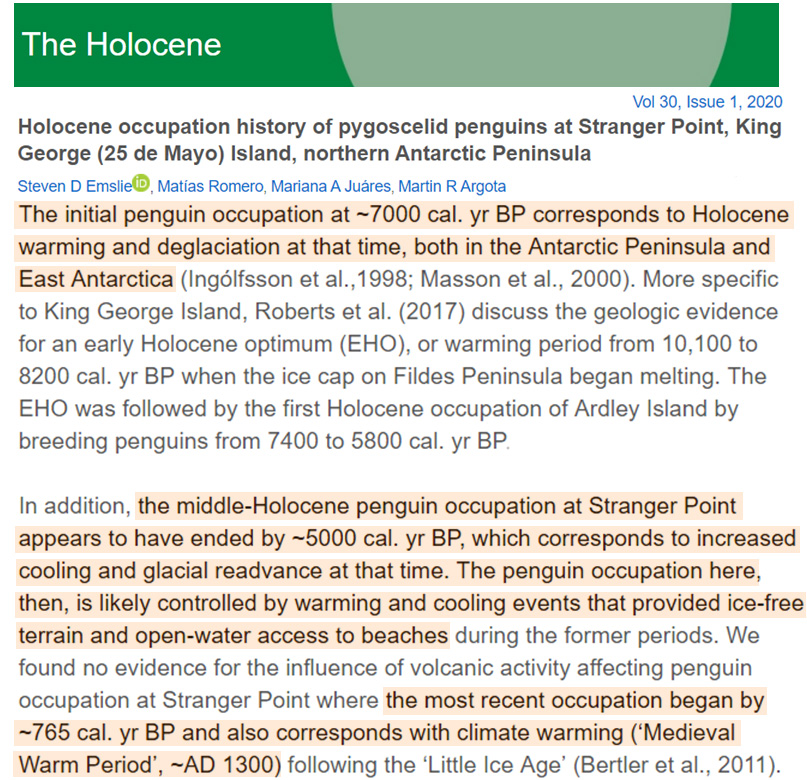
Here, we evaluated transgenerational effects of pH on byssal threads secreted by M. senhousia, and compared byssus performance in absence versus presence of predators. If no predation occurred, neither pH nor transgenerational exposure significantly affected the number, length and diameter of byssal threads. Under predation risk, mussels, even exposed to low pH, significantly enhanced byssus production. In particular, individuals originating from parents grown under low conditions produced significantly more, longer and stronger byssal threads compared with those spawn from parents exposed to high pH, demonstrating positive transgenerational effects which can confer mussel byssus resilience at low pH. … Our findings demonstrate the remarkable ability of highly invasive fouling mussel species to respond plastically and adapt behaviorally to low pH and hence provide important implications for linking marine biofouling, biological invasion, and coastal acidification.
Wound healing in an elasmobranch fish is not impaired by high‐CO2 exposure … [W]ound healing rates may not be strongly impacted by ocean acidification.
Here, we compared biofilm bacterial communities on intertidal cobbles/boulders and bedrock along a seawater CO2 gradient off Japan. Samples sequenced for 16S rRNA showed differences in bacterial communities with different pCO2 and between habitat types. In both habitats, bacterial diversity increased in the acidified conditions. Differences in pCO2 were associated with differences in the relative abundance of the dominant phyla. However, despite the differences in community composition, there was no indication that these changes would be significant for nutrient cycling and ecosystem function. As well as direct effects of seawater chemistry on the biofilm, increased microalgal growth and decreased grazing may contribute to the shift in bacterial composition at high CO2, as documented by other studies. Thus, the effects of changes in bacterial community composition due to globally increasing pCO2 levels require further investigation to assess the implications for marine ecosystem function. However, the apparent lack of functional shifts in biofilms along the pCO2 gradient is a reassuring indicator of stability of their ecosystem functions in shallow ocean margins.
In this study, fore reef coral communities were exposed to high pCO2 for a year to explore the relationship between net accretion (Gnet) and community structure (planar area growth). … These results suggest that skeletal plasticity modulates the effects of reduced Gnet at high pCO2 on planar growth, at least over a year. The low sensitivity of the planar growth of fore reef corals to the effects of ocean acidification (OA) on net calcification supports the counterintuitive conclusion that coral community structure may not be strongly affected by OA.
In this study, core samples of Schrenk spruce were collected in the Sayram Lake Basin, Xinjiang. Tree-ring radial growth and long-term intrinsic water-use efficiency (iWUE) chronologies were established based on standard tree-ring width and stable carbon isotope methods. The relationships between atmospheric CO2 concentrations, climate, radial growth, and iWUE were analyzed. Our results indicate that the iWUE [long-term intrinsic water-use efficiency] of trees in this region has continued to rise rapidly but that radial growth has not increased over the past 160 years.
[C]ontrary to these predictions, CO2-treated fish excelled at extracting oxygen from the water and outperformed the low-CO2 group in terms of hypoxia tolerance. When Montgomery took a closer look at the fish’s blood, he found no difference in blood pH between the treatments, indicating a remarkable capacity of the seabass to counteract the acidifying effect of elevated CO2. .. In European seabass it appears that the combined condition of a decreasing oxygen level and an increasing CO2 level in the water, as is found in nature, improves hypoxia tolerance. … [F]or seabass that find themselves gasping for oxygen, the natural rise in CO2 that comes with aquatic hypoxia may actually save lives.
Ocean acidification and ocean warming (OAW) are simultaneously occurring and could pose ecological challenges to marine life, particularly early life stages of fish that, although they are internal calcifiers, may have poorly developed acid-base regulation. This study assessed the effect of projected OAW on key fitness traits (growth, development and swimming ability) in European sea bass (Dicentrarchus labrax) larvae and juveniles. Starting at 2 days post-hatch (dph), larvae were exposed to one of three levels of PCO2 (650, 1150, 1700 μatm; pH 8.0, 7.8, 7.6) at either a cold (15°C) or warm (20°C) temperature. Growth rate, development stage and critical swimming speed (Ucrit) were repeatedly measured as sea bass grew from 0.6 to ~10.0 (cold) or ~14.0 (warm) cm body length. Exposure to different levels of PCO2 had no significant effect on growth, development or Ucrit of larvae and juveniles. At the warmer temperature, larvae displayed faster growth and deeper bodies. Notochord flexion occurred at 0.8 and 1.2 cm and metamorphosis was completed at an age of ~45 and ~60 days post-hatch for sea bass in the warm and cold treatments, respectively. Swimming performance increased rapidly with larval development but better swimmers were observed in the cold treatment, reflecting a potential trade-off between fast grow and swimming ability. A comparison of the results of this and other studies on marine fish indicates that the effects of OAW on the growth, development and swimming ability of early life stages are species-specific and that generalizing the impacts of climate-driven warming or ocean acidification is not warranted.
In recent years, increasing horror stories about the polar bear have emerged in media discourse: the polar bears is on the brink of extinction; the polar bear is starving due to the effects of climate change; or the polar bear invades human settlements in search for food. As we have seen in Chap. 2, the realities are far more complex. The Arctic Biodiversity Assessment (ABA), for instance, has found that of the 19 distinct polar bear populations all over the Arctic, seven are declining, four are stable, one is increasing, and the status of the remaining seven is unknown The claim of a declining polar bear is therefore imprecise. Similarly, the rather recently circulating image of a starving polar bear allegedly due to climate change caused high waves in social media. However, an extremely skinny polar bear in search for food can have numerous reasons and the causes for such physical state can also be related to disease or other factors. However, such emotional charging of the polar bear does certainly not miss its mark and attempts have been made to further protect this species from any human exploitation. … The IUCN lists the polar bear as ‘vulnerable’ and the overall population is estimated somewhere between 19,000–30,000 bears. Whether or not the overall trend is increasing or declining is unknown.
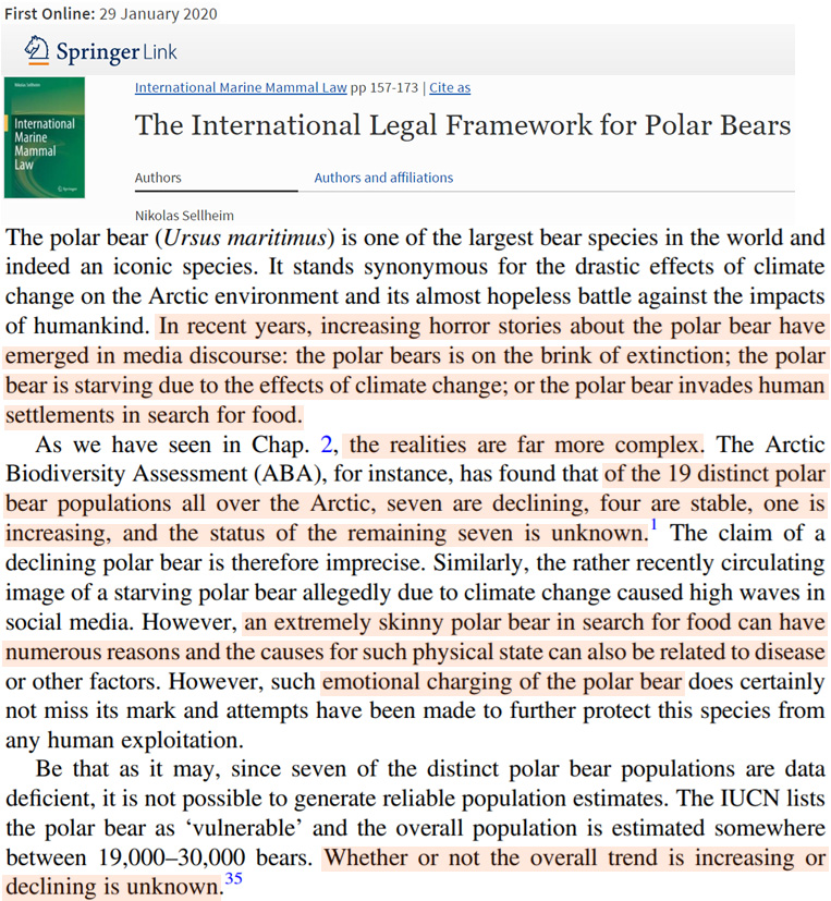
Fatty acid-based diet estimates suggest ringed seal remain the main prey of southern Beaufort Sea polar bears despite recent use of onshore food resources … Temporal trends analysis did not show clear increases or decreases in proportional consumption of any prey species [2004-2016] other than beluga, which were uncommon in the diet, despite significant interannual variation for all prey in the diet. … The effect for melt season was not significant for any individual prey (p > .10). Significant main effects on SB polar bear diet estimates were not seen for the 15% threshold (F1, 497 = 2.23, p = .06). Interaction terms were not significant in models using the ice metrics (p > .54). … We found that the diet estimates (43.6 ± 1.0% ringed seal, 21.8 ± 1.2% bearded seal, 14.8 ± 0.6% seabird, and 15.2 ± 0.8% bowhead and 4.6 ± 0.6% beluga) were very similar to the original estimates.
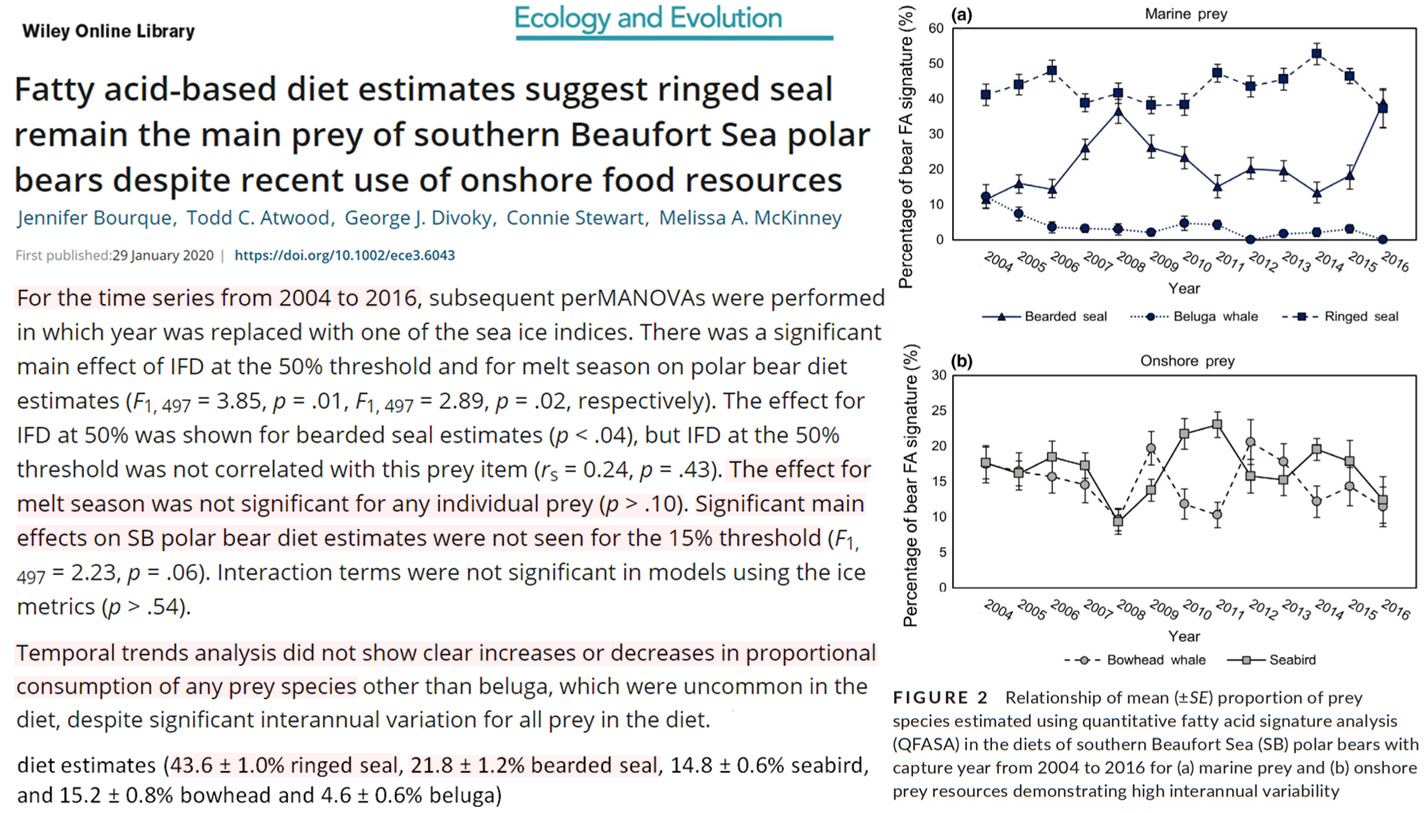
Bears in our study reached their lowest body condition in April or May. The highest adipose tissue lipid content was in the autumn (August–October), exceptin Baffin Bay where bears reached their highest body condition in January. The observed seasonal trends in body condition suggest that polar bears are actively feeding throughout late spring and early summer, corresponding with the availability of seal pups (e.g. Pagano et al., 2018; Stirling & McEwan, 1975; Stirling & Øritsland, 1995) and mature seals hauling out on the ice to moult (Kelly et al., 2010; Stirling, 2002; Stirling & Øritsland, 1995). … The increase in body condition after break‐up date was somewhat unexpected and suggests that polar bears may continue to feed as sea ice deteriorates to maximize energy gain. In Baffin Bay, Laidre et al. (2018) suggested that bears remain on sea ice over the continental shelf in July and early August to increase hunting opportunities.
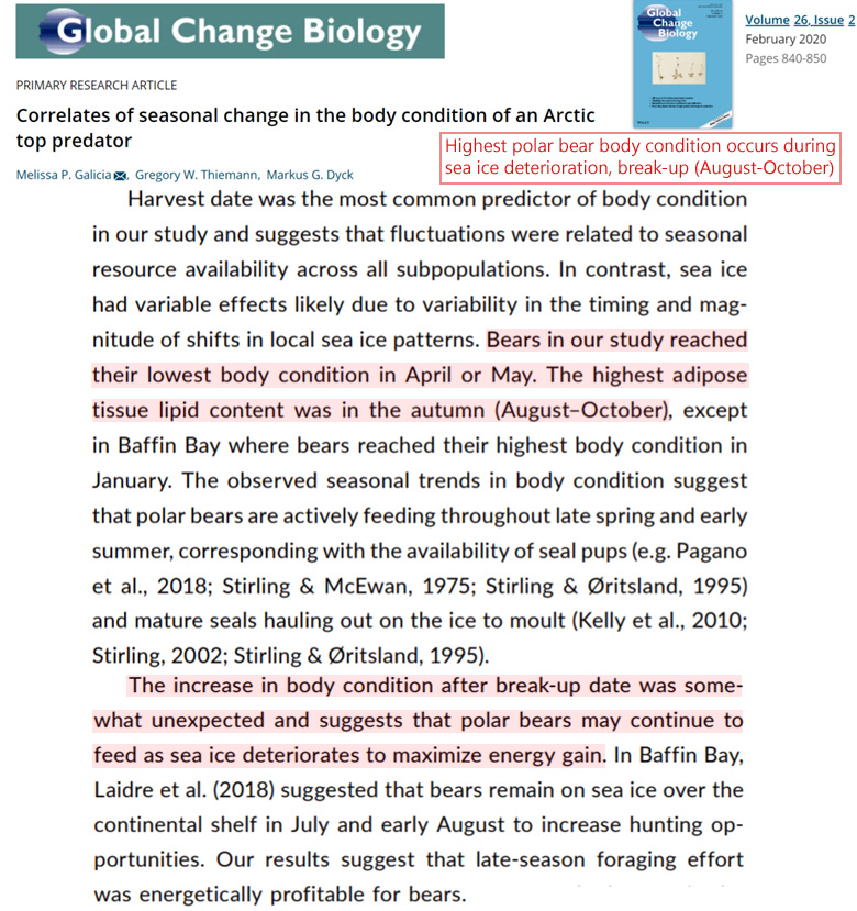
Elevated CO2: Greens Planet, Higher Crop Yields
Vegetation models suggest that CO2 fertilization is the main driver of greening on the global scale, with other factors being notable at the regional scale. Modelling indicates that greening could mitigate global warming by increasing the carbon sink on land and altering biogeophysical processes, mainly evaporative cooling.
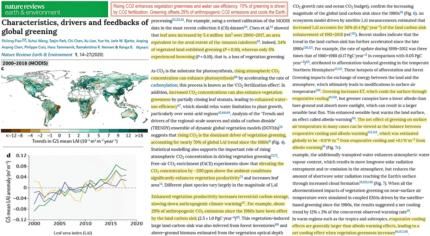
Elevated CO2 level (550 ppm) increased yield by 15.1% and 16.7% over ambient in wheat and by 21.1% and 21.9% in chickpea (p ≤ 0.05) during the first and second years of the study. Nitrogen content in wheat grains decreased under elevated CO2 concentration. Chickpea, being a leguminous crop, showed no change in grain N content. However, higher biomass and grain yield resulted in higher N uptake in both the crops under elevated CO2 level.
Greening Hiatus in Eurasian Boreal Forests Since 1997 Caused by a Wetting and Cooling Summer Climate … The Eurasian boreal forest ecosystem is a strong sink in the global carbon cycle. Satellite observations show significant change in the ecosystem in recent decades, specifically an increase in vegetation productivity since 1982 and a hiatus after 1997. Previous studies attributed this enhanced vegetation growth (also known as greening) to air temperature increases and a longer growing season, and the recent greening hiatus as a result of a warmer and drier climate. However, using satellite data, we found observational evidence that increases in summer peak growth dominated the overall greening trend and that a wetting and cooling climate during the peak growing season was the primary cause of the hiatus.
Increasing LUE [light use efficiency] (due to rising atmospheric CO2 concentration) and green vegetation cover were the primary controls of modelled GPP trends across sites. Global GPP [gross primary production] simulated by the same model increased by 0.46 ± 0.09 Pg C yr–2 during 1982–2016. … These findings strengthen the evidence that rising LUE [light use effciency] due to rising CO2 level and increased green vegetation cover (fAPAR) are the main causes of increasing GPP [gross primary production], and thereby, the terrestrial carbon sink.
Vegetation is a key regulator of land-atmosphere exchanges of heat, mass, and momentum (1, 2). Satellite records of leaf area index (LAI), a measure of the aboveground vegetation abundance, indicate widespread increasing trends since the 1980s (3), due to warming (4, 5), CO2 fertilization (6), and land management (7, 8). The Earth greening directly affects the surface energy budget through influencing various biophysical factors: (i) albedo (α), which controls the fraction of solar radiation absorbed by the surface; (ii) aerodynamic resistance (ra), which characterizes the efficiency of turbulent transfer of heat and water vapor; (iii) surface resistance (rs), which is the additional resistance to water vapor transport through the soil and the pores on leaves; and (iv) emissivity (ε), which is the effectiveness of a surface in emitting and absorbing longwave radiation. Changes in these biophysical factors can strongly affect the radiometric land surface temperature (LST). … The sensitivity of LST to LAI diagnosed from Community Land Model Version 5 (CLM5) outputs indicates a cooling effect due to the Earth greening globally (Fig. 1A).
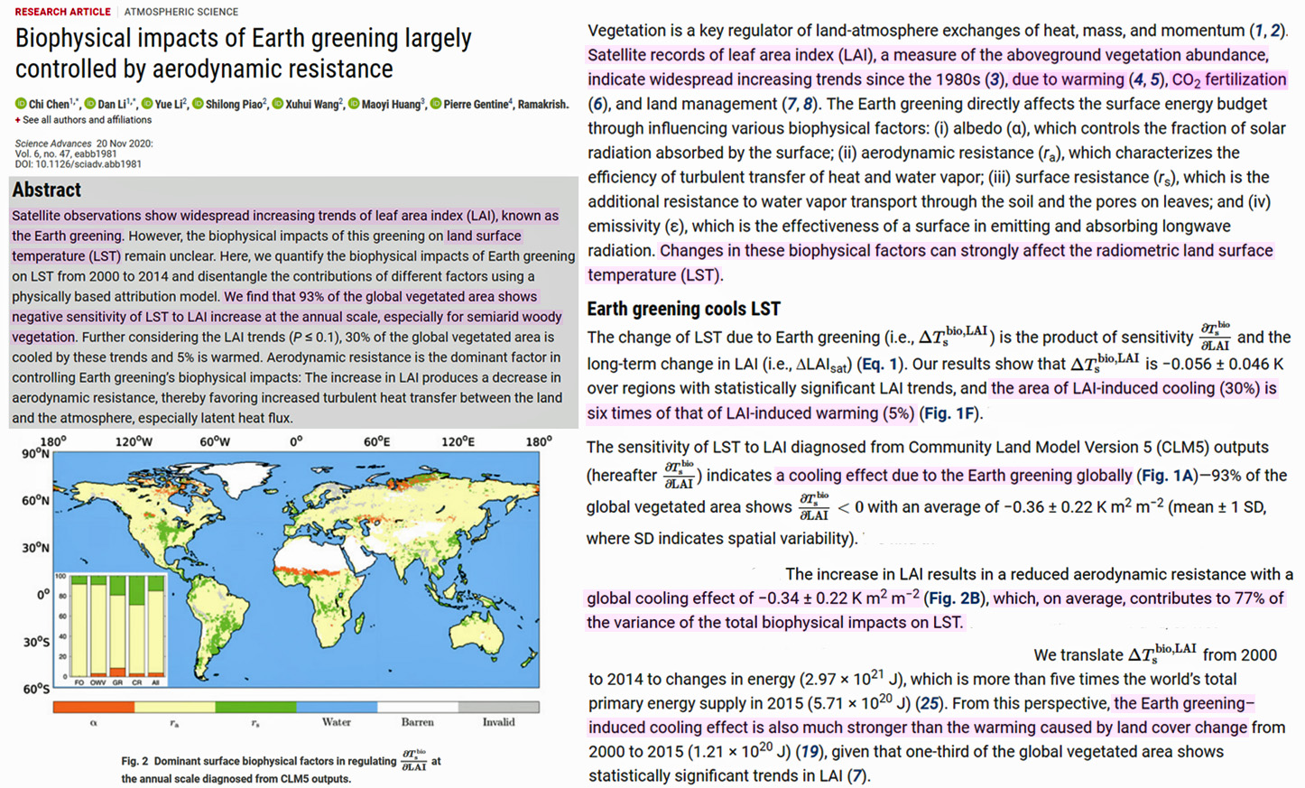
[D]oubled CO2 concentration which significantly increased the yield of cherry tomatoes (Solanum lycopersicum L.), i.e., up to 38% … CO2 fertilization…improved quality and increased the yield of cherry tomatoes.
Elevated air [CO2] improves photosynthetic performance and alters biomass accumulation and partitioning in drought-stressed coffee plants … Our results demonstrate that elevated [CO2] improved carbon assimilation rates (>60 %) with unaltered stomatal conductance and no signs of photosynthetic downregulation. This was accompanied by increases in water-use efficiency, respiration rates and biomass accumulation regardless of watering, and decreased photorespiration rates and oxidative pressure under drought. Improved growth under elevated [CO2] was more evident under drought than under full irrigation, and was unlikely to have been associated with global changes on hormonal pools, but rather with shifts on carbon fluxes. Finally, elevated [CO2] promoted key allometric adjustments linked to drought tolerance, e.g., more biomass partitioning towards roots with greater root length. Collectively, our results offer novel and timely information on the mitigating ability of elevated [CO2] on the photosynthetic performance and growth of coffee plants under drought conditions.
Growth and biomass were significantly enhanced by elevated CO2 and temperature. … It is concluded that the effect of elevated CO2 and temperature improved total above-ground plant biomass followed by FATI at both dates of observations. Total dry biomass including root was higher in FACE + FATI and FATI over ambient at 140 and 280 DAE, respectively. Free air temperature increase (FATI) and VC treated plants recorded 45.90% and 20.70%, higher hypericin content over ambient, respectively. Plant phenology was advanced in FACE. Consequently, the combined impact of CO2 and temperature brought about better development and yield of H. perforatum. Increased temperature alone improved the hypericin content.
Several lines of evidence point to an increase in the activity of the terrestrial biosphere over recent decades, impacting the global net land carbon sink (NLS) and its control on the growth of atmospheric carbon dioxide (ca). Global terrestrial gross primary production (GPP)—the rate of carbon fixation by photosynthesis—is estimated to have risen by (31 ± 5)% since 1900, but the relative contributions of different putative drivers to this increase are not well known. Here we identify the rising atmospheric CO2 concentration as the dominant driver. We reconcile leaf‐level and global atmospheric constraints on trends in modeled biospheric activity to reveal a global CO2 fertilization effect on photosynthesis of 30% since 1900, or 47% for a doubling of ca above the pre‐industrial level. Our historic value is nearly twice as high as current estimates (17 ± 4)% that do not use the full range of available constraints. Consequently, under a future low‐emission scenario, we project a land carbon sink (174 PgC, 2006–2099) that is 57 PgC larger than if a lower CO2 fertilization effect comparable with current estimates is assumed. These findings suggest a larger beneficial role of the land carbon sink in modulating future excess anthropogenic CO2.
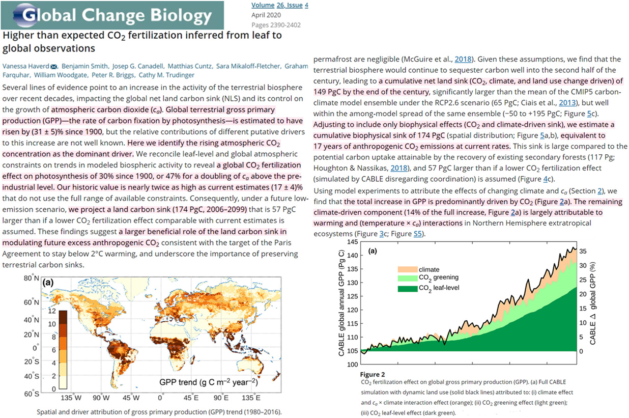
Elevated CO2 (eCO2) stimulates plant growth and photosynthesis, which affect root deposition, leading to altered structure and function of the root microbiome. We studied the effect of eCO2 on wheat-root microbiome composition and plant development, with an emphasis on denitrifying communities. Wheat plants were grown in a greenhouse with continuous fertigation for 6 weeks under ambient CO2 (400 ppm) or eCO2 (850 ppm). … eCO2 had a significant impact on abundance of the studied denitrifying genes, particularly during the late stages of wheat growth before spike formation. Moreover, eCO2 had a significant impact on N2O-reducing community structure in roots. … In summary, it is suggested that eCO2 may change root microbiome, enhance wheat development and N demand without an increase in N2O emission.
Here we combine satellite measurements of greening with a 135 year record of plant C and nitrogen (N) concentrations and stable isotope ratios (δ13C and δ15N) in the Northern Great Plains (NGP) of North America to examine N constraints on greening. We document significant greening over the past two decades with the highest proportional increases in net greening occurring in the dries and warmest areas. In contrast to the climate dependency of greening, we find spatially uniform increases in leaf‐level intercellular CO2 and intrinsic water use efficiency that track rising atmospheric CO2.
Global Warming Reduces Mortality. Cold Kills.
Gasparrini et al. (2015) studied 74,225,200 deaths in various periods across 384 worldwide locations between 1985 and 2012, and found that 7.29% of deaths were attributable to cold, while there were only 0.42% attributable to heat. … During January 22–24, 2016, a cold wave severely influenced various cities in East Asia within a very short period, resulting in a sudden drop in air temperature and a consequence of socioeconomic loss. In general, the China Meteorological Administration has found that 1.18 billion people living in Eastern China suffered from a sudden drop in average temperature of greater than 6 C during the event (Qian et al., 2018). … We found that the cold wave induced a prolonged effect on mortality across the city for 5 weeks.
In this paper, the Lamb Weather Type synoptic classification is used to examine the relationship between daily mortality and weather patterns across nine regions of England. Analysis results revealed that the population in England is more susceptible to cold weather. Furthermore, it was found that the Easterly weather types are the most hazardous for public health all-year-long; however, during the cold period, the results are more evident and spatially homogenous.
Warmer Temps Are “More Favorable” To Humans
[T]he highest biomass and biodiversity is present in tropical rainforests, and the least in cold polar regions (Brown, 1990, 2013; Kraft et al., 2011). Thus, higher temperatures than currently existing on Earth seem to be more favorable. … Thus, a slightly higher temperature, perhaps by 5°C—similar to that of the early Carboniferous time period—would provide more habitable conditions until some optimum is reached. As pointed out earlier, a higher water content in the form of more moisture and more clouds would be beneficial in principle, with the rainforests on Earth being again a good example. A higher water content (absolute humidity) in the atmosphere would also provide more protection from UV irradiation.
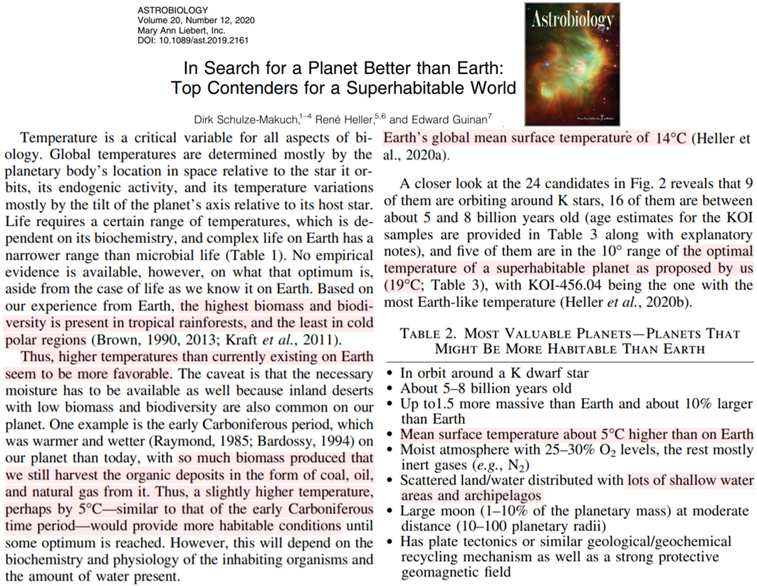
During the cold dry period between 5600 and 5000 yr BP, only 65 human cultural sites have been found (Wang, 2003). During the warm and humid period from 4200 to 3800 yr BP, 632 cultural sites were found (Jia et al., 2008). Therefore, it can be estimated that there were 1.1 cultural sites per 100 years in the cold and dry period, but 15.8 cultural sites per 100 years in the warm and humid period. This indicates the greater development of cultural sites during warm and wet periods than during cold and dry periods.
No Increasing Trends In Intense Hurricanes
Because a change in the frequency (number/year) of hurricanes could be a result of climate change, we analyzed the historical record of Atlantic basin and US landfalling hurricanes, as well as US continental accumulated cyclone energy to evaluate issues related to trend detection. Hurricane and major hurricane landfall counts exhibited no significant overall trend over 167 years of available data, nor did accumulated cyclone energy over the continental USA over 119 years of available data … Storm energy data 1900–2018 over land were also analyzed. The trend was again zero. … Atlantic basin all storms and major storms (1950–2018) did not exhibit any trend over the whole period or after 1990. Major storms 1950–1989 exhibited a significant downward trend.
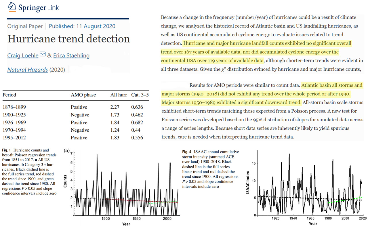
No Increasing Trend In Drought Frequency, Severity
Here we use a long-term (1870–2018) data to identify the top five (“deadly”) meteorological/hydrological droughts based on overall severity score in the last century and half period. Out of a total of 18 meteorological droughts, the deadly droughts occurred in 1899, 1876, 2000, 1918, and 1965. Similarly, the deadly hydrological droughts occurred in 1899, 2000, 1876, 1965, and 1918 during 1870–2018. All the five deadly droughts were associated with the positive phase of El Nino Southern Oscillations (ENSO). 2015–2018 drought was the longest duration in the entire record (1870–2018) but was not among the most severe droughts.
Our regional tree‐ring record is strongly correlated with the November–April self‐calibrated Palmer drought severity index and enabled us to reconstruct drought variability for the period 1802–2016. The reconstruction explained 46.5% of the actual self‐calibrated Palmer drought severity index variance. Over the past two centuries, we detected one extreme (1812) and six severe drought years (1810, 1811, 1816, 1852, 1887, and 1980). Dry periods coincided with six major famines that occurred in India. Spatial correlation analyses revealed that drought occurrence is linked to broader‐scale atmospheric circulations of the Pacific and Indian Oceans, especially during the positive phase of the El Niño–Southern Oscillation. Our reconstruction provides a useful historical perspective for assessing adaptation measures intent on mitigating future drought impacts in Myanmar.
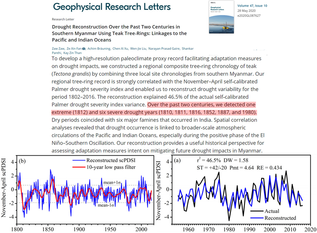
Results showed that years with high drought magnitude ranged from 1920−22, 1926−29, 1942−46 and 1947−51 with values corresponding to 2.2, 3.2, 3.4 and 2.6, respectively while years with low drought magnitude ranged from 1930−31, 1988−89 and 2001−02 with values as 0.2, 0.12 and 0.15, respectively. The longest droughts occurred from 1926−29, 1937−41, 1942−46, 1947−51, 1952−56, and 1958−61 with values in years as 3, 4, 4, 4, 4, and 3 years, respectively, while the shortest droughts occurred in time period of 1 year and ranged from 1930−31, 1964−65, 1979−80, 1981−82, 1983−84, 1988−89, 1991−92, 1993−94, 1996−97 and 2001−02.
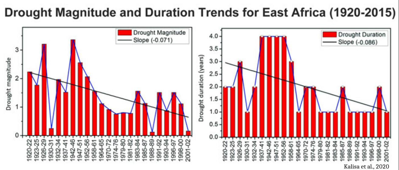
Natural CO2 Emissions A Net Source, Not A Net Sink
The system is an atmospheric CO2 source in spring and winter, near neutral in early summer, a large sink in late summer after WSR, and finally a large atmospheric CO2 source in autumn. Discharge events and seasonality jointly affect estuarine CO2 flux. High CO2 sequestration in summer is due mainly to a combination of high water temperature, chlorophyll a levels, dissolved inorganic carbon, and solar radiation and low turbidity, discharge, and chemical oxygen demand (COD) after WSR. WSR supports the high gross primary productivity rate which exceeds the increase in ecosystem respiration. .. Although the YRE, as a whole, is a source of atmospheric CO2, the amount of CO2 released is lower than the average estuarine value of mid-latitude regions.
We examined the dynamics of dissolved inorganic carbon (DIC) and pH in the Pearl River Estuary (PRE) and the adjacent northern South China Sea (NSCS) shelf in summer, aiming for a better understanding of the interaction between eutrophication, hypoxia, and ocean acidification. … In combination with stable carbon isotopic compositions, we found biological production and CO2 outgassing to be responsible for DIC deficits in surface waters, while degradation of organic matter (OM) accounted for DIC additions in bottom waters. The PRE‐NSCS plume system as a whole served as a net source of atmospheric CO2 from the perspective of Lagrangian observations, because strong CO2 outgassing in the inner estuary overwhelmed the CO2 uptake in the plume despite strong phytoplankton blooms.
Over the last five decades, numerous studies have been developed to investigate the Gulf of California (GC) in terms of atmospheric circulation and physical and biological oceanography. The GC is recognised by its high productivity due to high nutrient availability in the euphotic zone driven by advection, thermohaline circulation, vertical mixing, and coastal upwelling (Alvarez‐Borrego & Lara‐Lara, 1991; Badán‐Dangon et al., 1985; Lavín & Marinone, 2003; Roden, 1964). Nowadays, as part of a coastal upwelling zone, the gulf acts as a net source of CO2 to the atmosphere (Rodríguez‐Ibáñez et al., 2013).
A carbon cycle model is built to describe the behavior of carbon materials in the Pearl River Estuary (PRE), China. The distributions and transformations of dissolved inorganic carbon (DIC), dissolved organic carbon (DOC), and particulate organic carbon (POC) are simulated in the water column and sediment for the year 2006. The terrestrial carbon input is the dominant factor that determines the seasonal variation of carbon, while physical and biochemical processes contribute to the spatial‐temporal circulation of carbon. The simulation results reveal that the PRE acts as a net source for atmospheric CO2 throughout the year, and it buffers the export of DIC from the river and sediment to the adjacent system via the DIC consumption by primary production. As a consequence of biochemical processes, the PRE exports more organic carbon to the sediment and adjacent marine ecosystems than the amount that it receives from upstream river reaches.
A carbon mass-balance budget for an entire lake catchment in West Greenland. … CO2 evasion from the lake surface and sediment burial accounts for 57% and 38% of aquatic export/storage, respectively (or 0.8% and 0.5% of total export/storage), and Two-Boat Lake acts as a net source of carbon to the atmosphere.
Reforestation Cools The Surface Multiple Degrees
This study quantified the regional temperature effects of recent land cover changes in Europe with a regional climate model, and, by directly connect ing local climate impacts to individual LCCs, it expands the scientific basis towards a better understanding of the potential land-climate interactions for more climate-oriented land management strategies. Land-climate interactions are strictly coupled to societal developments, especially in terms of urbanization and cropland extension/contraction. Reduction of urban sprawling will bring temperature benefits across all Europe. … We found an annual average temperature change of −0.12 ± 0.20 °C (mean ± standard deviation), with −0.42 and +0.22 °C as the 5th and 95th percentile (Fig. 2a), respectively, from recent LCCs in Europe. An average cooling is consistently spread in the southern, central and western part of Europe, whereas warming occurs in eastern Europe. Relatively little changes in temperature are observed in northern Europe (Scandinavia), where relatively limited land transitions took place. … At an average European level, transitions from forest to any other land cover class show mean warming effects, including conversion of forests to cropland (+0.15 ± 0.03 °C), grassland (+0.23 ± 0.06 °C), and urban (+0.27 ± 0.06 °C). Urban sprawling always shows warming contributions, irrespective of the type of previous land cover.
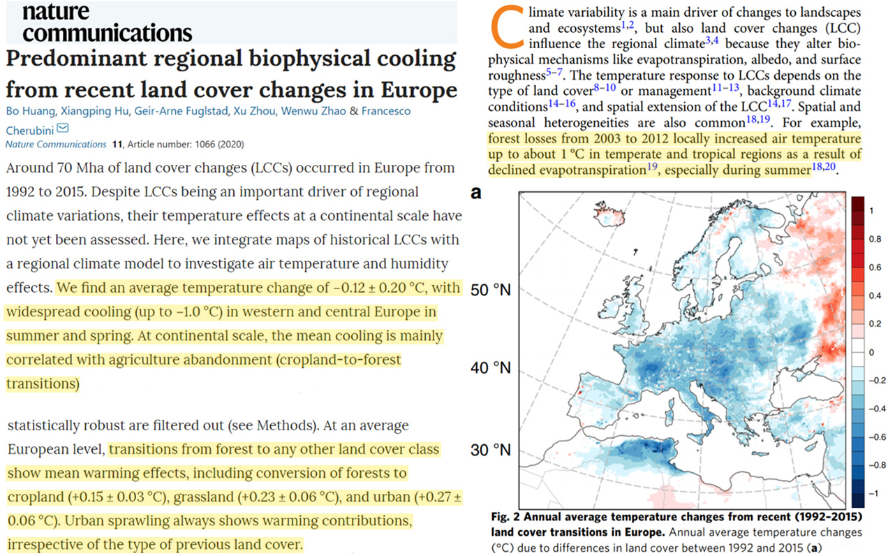
During growing season daytime periods, T surf is 4–6 °C cooler, and T aero and near‐surface T extrap are 2–3 °C cooler, in the forests relative to the grassland. During the dormant season, daytime differences are smaller but still substantial. At night, differences in T aero are small, and near‐surface T extrap is warmer over forests than grasslands during the growing season (by 0.5 to 1 °C). Finally, the influence of land cover on T extrap at the interface between the surface and mixed layer is small. Overall, reforestation appears to provide a meaningful opportunity for adaption to warmer daytime Ta in the southeastern United States, especially during the growing season. … Reforestation—the process of reestablishing trees where they once dominated—has long been viewed as a strategy to remove CO2 from the atmosphere. Recently, attention has focused on understanding if reforestation also offers a direct temperature cooling benefit. By using more water (a cooling process) and increasing the transfer of heat energy away from the surface, forests may offer a meaningful opportunity for local climate mitigation and adaptation. Evidence is mounting that indeed, in the temperature and tropical zones, the surface of forests is cooler than grasslands and croplands. However, due to confounding effects of forest canopies on wind and temperature profiles near the surface, it has previously been hard to assess if forests also cool the air. Here we present a new approach that accounts for canopy effects, allowing for a more direct assessment of the potential for reforestation to cool near‐surface air temperature. Using a case study from the North Carolina Piedmont, we find that while the air cooling effect of forests is not a large as the surface cooling effect, it is still on the order of 2–3 °C during summer daytime periods—times when the need for climate adaptation strategies are particularly pressing.
Mass Extinctions Due To Global Cooling
Therefore, combining the interpretations of our data with previous publications suggest that the mechanism for the first extinction pulse of the LOME [Late Ordovician Mass Extinction] involved a major eustatic sea-level drop of ≥100 m, global cooling, and glaciation. Glacioeustatic sea-level drawdown would have drained widespread epeiric seaways globally, thus eliminating vast areas of habitable shallow marine environments in the Hirnantian (Sheehan, 2001). This dramatic reduction in marine shelf area would have led to the extinction of many endemic communities via habitat loss and carrying capacities of the remaining environments being exceeded (Brenchley et al., 2001). Recent sea-level reconstructions from sedimentary successions on Baltica, including both Aizpute-41 and Röstånga-1drill cores, suggest multiple regressive events within the Hirnantian (Kiipli and Kiipli, 2020). Sea-surface temperature proxies record a rapid cooling by ~5 °C during the Hirnantian and are consistent with this climate-driven first extinction pulse scenario (Trotter et al., 2008; Finnegan et al., 2011).
The eruption of Emeishan lava in southwestern China and northern Vietnam is considered to be a contributing factor to the Capitanian mass extinction and subsequent global cooling event, but the duration of volcanism is uncertain. The difficulty in assessing the termination age is, in part, due to the lack of high-precision age data for late-stage volcanic rocks. The Tu Le rhyolite of northern Vietnam is the most voluminous silicic unit of the Emeishan large igneous province (ELIP) and is spatially associated with the Muong Hum and Phan Si Pan hypabyssal plutons. Chemical abrasion–isotope dilution–thermal ionization mass spectrometry U-Pb dating of zircons from the Tu Le rhyolite (257.1 ± 0.6 Ma to 257.9 ± 0.3 Ma) and Muong Hum (257.3 ± 0.2 Ma) and Phan Si Pan (256.3 ± 0.4 Ma) plutons yielded the youngest high-precision ages of the ELIP yet determined. The results demonstrate that Emeishan lavas erupted over a period of ∼6 m.y,. with plutonism ending shortly thereafter. Thus, it is possible that Emeishan volcanism contributed to global cooling into the middle Wuchiapingian. It appears that these rocks represent a distinct period of ELIP magmatism, as they are young and were emplaced oblique to the main north-south–trending Panxi rift.
Doubling Atmospheric Pressure Warms Earth 7-10K
When the surface air pressure is increased from 1.0 to 2.0 bar, the global-mean surface temperature increases by 10 K, and all the sea ice melts (green line in Fig. 5a). When the surface air pressure is further increased from 2.0 to 4.0 bar, the global-mean surface temperature increases by 17 K. … The surface temperature at the equator rises by 10 K as the surface pressure is increased from 1.0 to 2.0 bar, while the polar surface temperature rises by 23 K. The main reason is the ice albedo feedback … The effect of halfing or doubling the surface pressure on the global-mean surface temperature is about 10 K or even as large as 17–84 K when the ice albedo feedback or water vapor feedback is strong (Table 1).
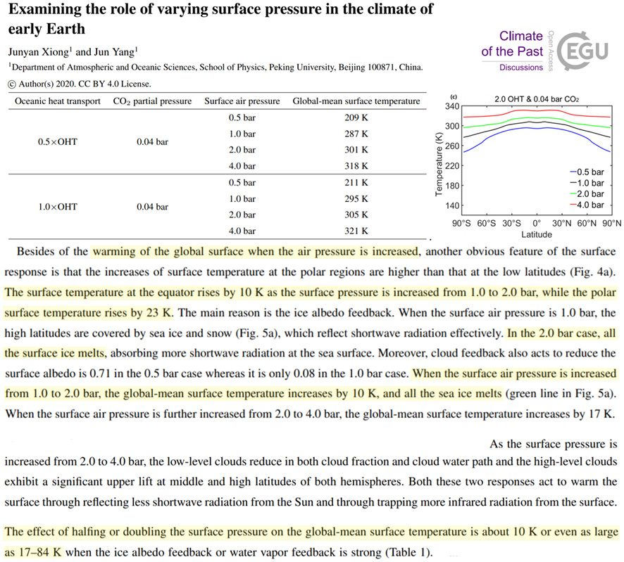
Xiong et al., 2020 (full paper)
Chemke et al. (2016) and CK17 suggested that the radiative effect of atmospheric mass caused changes in the tropospheric temperature gradient and atmospheric circulations. Their results provided valuable guidances, although the processes neglected in the idealized model (e.g., more realistic representation of convection and the cloud radiative effect, CRE) may modify the picture. Several GCM studies with sophisticated radiation and cloud physics under realistic configurations of orography have consistently suggested that a higher atmospheric mass leads to significant warming; for example, a doubling of atmospheric pressure produces a warming of ∼7 K (Charnay et al. 2013), and a pressure of 2.4 bar N2 leads to surface warming of 9.7 K (Wolf and Toon 2013).
Too big to fly? An engineering evaluation of the fossil biology of the giant birds of the Miocene in relation to their flight limitations, constraining the minimum air pressure at about 1.3 bar … The fossil biology of flight is one of the few options available for obtaining information on the density of past atmospheres. The giant birds of the Miocene, the 70 kg teratorn Argentavis magnificens and the giant Pelagornithidae with wingspans of 6.5 m or more, have long intrigued bird specialists, leading one researcher, Colin Pennycuick, to hypothesize that a higher air density may have been necessary for these birds to fly. To test this hypothesis, previous mass estimates and wing shapes of these birds are reviewed and the revised values used in the Flight 1.25 bird simulation program to investigate and quantify in engineering terms the limitations of flight in the present atmosphere as well as in hypothetical higher densities. The results indicate that Pennycuick was probably right: the available takeoff power for a gorged teratorn in an atmosphere of 1 bar is too low and attempts at level takeoff could involve a high risk of injury; The giant Pelagornithidae would have had enough power for takeoff, but flapping bone stress at 1 bar would also have been critical. Simulations indicate that for both birds, power and bone stress constraints are overcome at about 1.3 bar, also enhancing the dynamic soaring of the Pelagornithidae. This level of atmospheric pressure would imply a different climate than the present, but is consistent with the data on average global temperatures for the Miocene before the Late Cooling Events, as well as with the polar to equator temperature gradient.
Miscellaneous
Shin et al., 2020 CO2 changes lag temp changes by 870-1,500 years
However, the CO2 decrease did not always start at exactly the same time as the onset of the DO warming, and the lag itself varied. For example, during Marine Isotope Stage (MIS) 3, atmospheric CO2 maxima lagged behind abrupt temperature change in Greenland by 870±90 yrs. During MIS 5, the lag of atmospheric CO2 maxima with respect to abrupt temperature warming in the NH was only about 250±190 yrs (Bereiter et al., 2012). … During MIS 6d which corresponds to CDM 6d.1 and 6d.2, CO2 concentrations show a much slower increase over a duration of ~3.3 kyr. Here, CO2 lags behind the onset of the NH abrupt warming by 1,500±280 yrs and 1,300±450 yrs, respectively (1,400± 375 yrs on average).
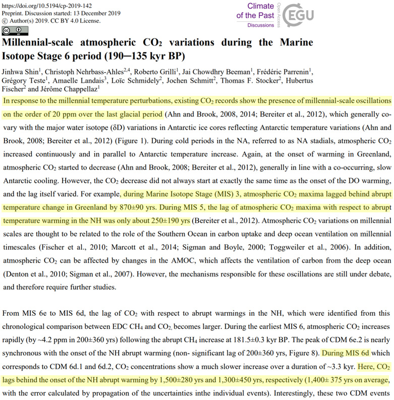
Ragazzola et al., 2020 Lower pH, more “acidic” water with 255 ppm CO2
Our inferred pH reconstruction for the Mediterranean Sea at 11.37 cal ka BP showed values similar to the present. In contrast, at 8.6 and 10.6 cal ka BP, all analysed species recorded lower pH compared to Recent specimens, contrary to what would be expected based on the lower atmospheric CO2 at that time (Monnin et al. 2004).
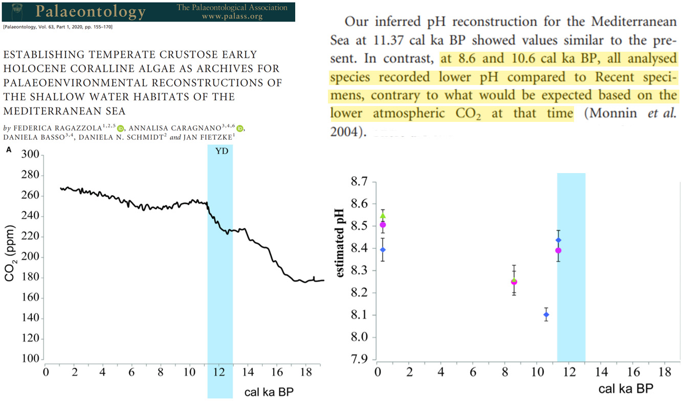
Mayhew et al., 2020 Global warming “little to do with so-called greenhouse gases”
It becomes rather obvious that a gas’s ability to absorb thermal energy should be based upon their heat capacities and not their infrared spectrums. At least not on the infrared spectrums in their current forms. … It has clearly been argued that blackbody/thermal phonons/photons are absorbed/radiated by all forms of matter, whether it be solid (both crystalline and amorphous), liquid, or even a polyatomic gas. The theoretical mistakes have been re-enforced by the subtraction of blanks in infrared spectrometry. Heat capacities clearly demonstrate that gases, liquids and solids (both amorphous and crystalline) all can, and will absorb/radiate their surrounding thermal/blackbody radiation, most often in rather similar manners. … The implication of the new understandings presented herein will be fundamental in any new understanding of thermodynamics. It also means that there exists a need to create new realistic models for climate change, models that recognize that global warming is due to man’s activities and have little to do with the so-called greenhouse gases.
Connolly et al., 2020 CO2 climate sensitivity could be much lower than IPCC’s claimed range
If the climate sensitivity to greenhouse gases implies a Transient Climate Response (TCR) of ≥ 2.5 °C or an Equilibrium Climate Sensitivity (ECS) of ≥ 5.0 °C then the 2015 Paris Agreement’s target of keeping human-caused global warming below 2.0 °C will have been broken by the middle of the century under BAU. However, for a TCR < 1.5 °C or ECS < 2.0 °C, the target would not be broken under BAU until the 22nd century or later. Therefore, the current Intergovernmental Panel on Climate Change (IPCC) “likely” range estimates for TCR of 1.0 to 2.5 °C and ECS of 1.5 to 4.5 °C have not yet established if human-caused global warming is a 21st century problem. … Moreover, as can be seen from Table 4, several studies have suggested that the climate sensitivity may be either higher or lower than the IPCC’s “likely” ranges. For instance, Zelinka et al. (2020) have noted that several of the latest CMIP6 Global Climate Models imply an ECS that is greater than 4.5 °C. On the other hand, Lindzen and Choi (2011) argue that the ECS is in the range 0.5–1.3 °C, with a most likely value of 0.7 °C [260], and both Monckton et al. (2015a) [216] and Bates (2016) [209] argue that the ECS is in the range 0.8–1.3 °C, with a most likely value of 1.05°C. All of these estimates are below the IPCC’s “likely” range. Meanwhile, some of us have argued in Soon et al. (2015) that the TCR is less than 0.44 °C, and that it is possible to explain all of the observed warming since at least 1881 in terms of natural climate change [152].
Wijngaarden and Happer, 2020 “at current concentrations, the forcings from all greenhouse gases are saturated”
[A]t current concentrations, the forcings from all greenhouse gases are saturated. The saturations of the abundant gases H2O and CO2 are so extreme that the per-molecule forcing is attenuated by four orders of magnitude with respect to the optically thin values. Saturation also supresses the forcing power per molecule for the less abundant greenhouse gases. … One greenhouse gas interferes with, and diminishes, the forcings of all others.
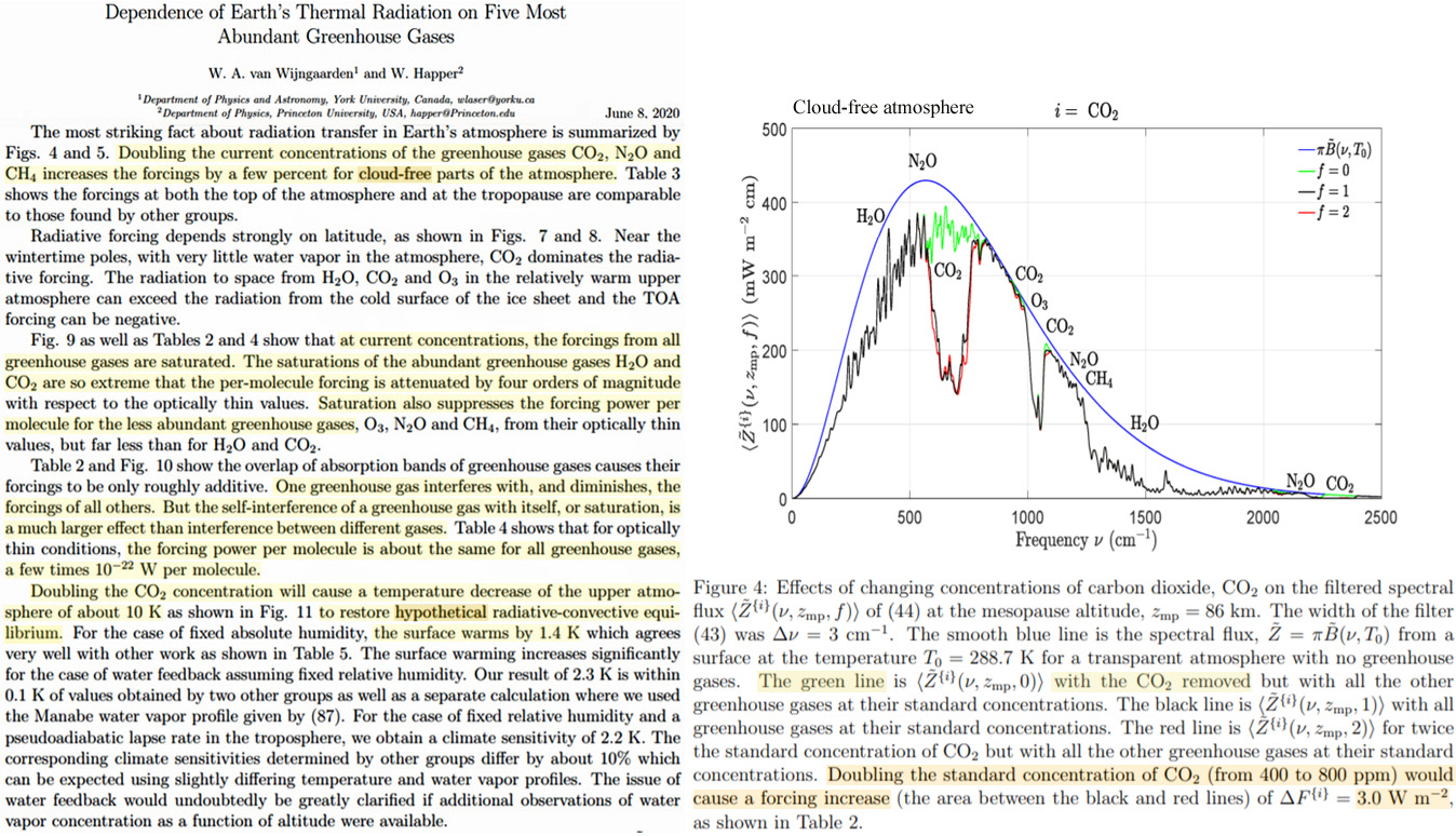
Niu et al., 2020 “violent” CO2 variations (-21 to +113 ppm) in hours predominantly driven by biological processes
Diurnal CO2bio showed violent variations (−20.9–113.3 ppm), with high values at night and low or negative values during the daytime. … CO2bio was the main contributor to diurnal CO2 variations over background level on the summer sampling days, and CO2bio concentrations were 8.5 ± 26.9 ppm higher than corresponding CO2ff concentrations on the summer sampling days, especially at night (15.3 ± 27.9 ppm).
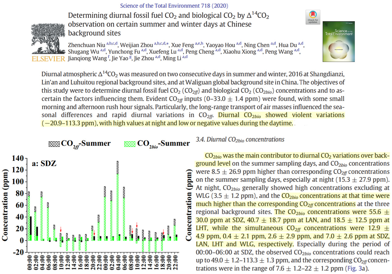
Bunbury et al., 2020 Egyptian Sahara wetter (trees, lakes), occupied, when globe is warmer
Holocene large lake development and desiccation: Changing habitats in the Kharga Basin of the Egyptian Sahara … Consideration of temperature proxy curves, for example, GISP2 from Greenland (Alley, 2000; Cuffey & Clow, 1997) in Figure 15 show that there have been many climate oscillations during the Holocene. We note from our results that periods of high global temperature are correlated with the episodes of reoccupation of the Kharga Basin [Sahara Desert] where the wetter the climate is, there is more extensive the reoccupation of the basin. Sedimentary evidence demonstrates that at some periods there was standing water that may have persisted for some decades (e.g., Wadi Bershama), at other times, drying lakebeds received sufficient water for trees to grow (e.g., Pot Playa).
Petryshyn et al., 2020 A not “plausible” 8- to 1,024-fold increase in CO2 required to explain past warming/extinctions
If the dendrolitic facies represent true background climate, then the CM records at least three temperature spikes of ~17ºC followed (at least twice) by a cooling and a return to background temperatures. Given a climate sensitivity of between 1.5 to 4.5ºC (IPCC, 2014), at least three atmospheric pCO2 increases on the order of 8- to 1024-fold (three to ten doublings) would be required to explain the CM temperature record. By way of comparison, Huynh and Poulsen (2005) modeled the end-Triassic climate at 2, 4, 6, and 8 times preindustrial pCO2, finding that global mean SSTs increased by only 5.4ºC over this pCO2 range (<10ºC for the paleo-Bristol region), short of the temperature increases recorded by the CM. T-J pCO2 reconstructions from fossil plant stomata and pedogenic carbonates indicate 1-4 instances of pCO2 doubling to quadrupling in association with the T-J transition (McElwain et al., 1999; Schaller et al., 2011; Schaller et al., 2012), well short of that required to explain our data. Moreover, the natural atmospheric CO2 relaxation timescale in models is on the order of 100s of kyr (Lord et al., 2015), which matches the observed timescales of T-J pCO2 drawdown from pedogenic carbonate records (Schaller et al., 2011; Schaller et al., 2012). Thus, each transition from laminated to dendrolitic facies would need to represent 100s of kyr, an order of magnitude longer than plausible given the depositional scenario (Ibarra et al., 2016; Ruhl et al., 2010). … Our results show multiple changes in temperature of ~17 ºC at the ETME interval, which we conclude, given the implausibility of other scenarios, must represent a strong seasonal temperature signal. This interpretation closely matches the local strength of seasonality in general circulation models (both this study and Huynh and Poulsen (2005), lending credence to our interpretations of the timescale represented by the proxy data. The exact mechanism for the ETME remains the subject of intense debate. While we cannot rule out a brief global-cooling event on timescales faster than the resolution of our record, we find no evidence for millennial-scale global cooling (Guex et al., 2016) following the initiation of CAMP volcanism. Additionally, we cannot resolve millennial-scale increases in temperatures in the region, implying that, at least locally, the initial extinction is not attributable to extreme warming.
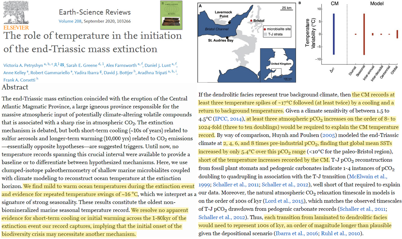


Recent Comments