A Warmer Past: Non-Hockey Stick Reconstructions
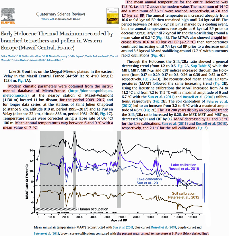
Martin et al., 2020 France max Holocene temps (14°C) were 7°C warmer than the modern value (7°C)
Modern climatic parameters were obtained from the instrumental database of Meteo-France at the nearby station of Mazet-Volamont (1130 m) located 11 km distant, for the period 2009-2017 … Temperature values were corrected using a lapse rate of 0.6°C/ 100 m. Mean annual temperatures vary between 6 and 9°C with a mean value of 7°C. … The mean annual temperature for the entire Holocene was 11.3°C, i.e. 4.1°C above the modern value. The maximum of 14°C and a minimum of 7.6°C were reached, respectively, at 7.8 and 1.7 kyr cal BP. … The last 200 years display an opposite trend … MAAT decreased by 3.1 and 3.3°C for the lake calibrations, Sun et al. (2011) and Russell et al. (2018), respectively, and 2.1°C for the soil calibration.
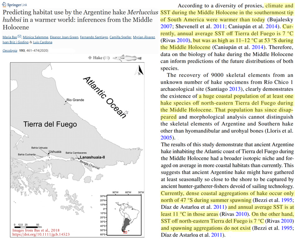
Bas et al., 2020 Southern South America SSTs 4-5°C “warmer than today”
According to a diversity of proxies, climate and SST during the Middle Holocene in the southernmost tip of South America were warmer than today (Bujalesky 2007; Shevenell et al. 2011; Caniupán et al. 2014). Currently, annual average SST of Tierra del Fuego is 7 °C (Rivas 2010), but was as high as 11–12 °C at 53 °S during the Middle Holocene (Caniupán et al. 2014).
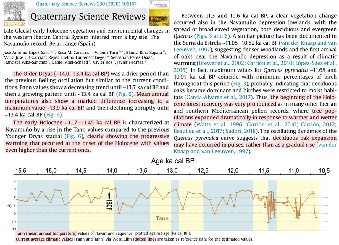
Lopez-Saez et al., 2020 Spain temps “even higher than the current ones” when Holocene began
The early Holocene ~11.7-11.45 ka cal BP is characterized at Navamuno by a rise in the Tann [mean annual temperature] values compared to the previous ~ Younger Dryas stadial (Fig. 6), clearly showing the progressive warming that occurred at the onset of the Holocene with values even higher than the current ones.
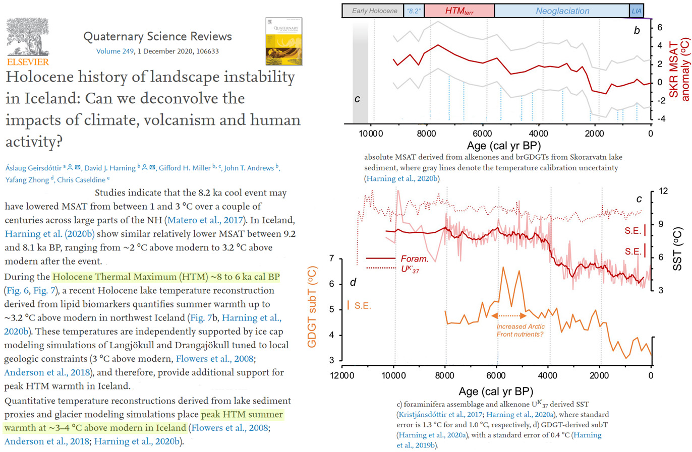
Geirsdóttir et al., 2020 Iceland “~3-4°C above modern”
Quantitative temperature reconstructions derived from lake sediment proxies and glacier modeling simulations place peak HTM summer warmth at ∼3–4 °C above modern in Iceland (Flowers et al., 2008; Anderson et al., 2018; Harning et al., 2020b).
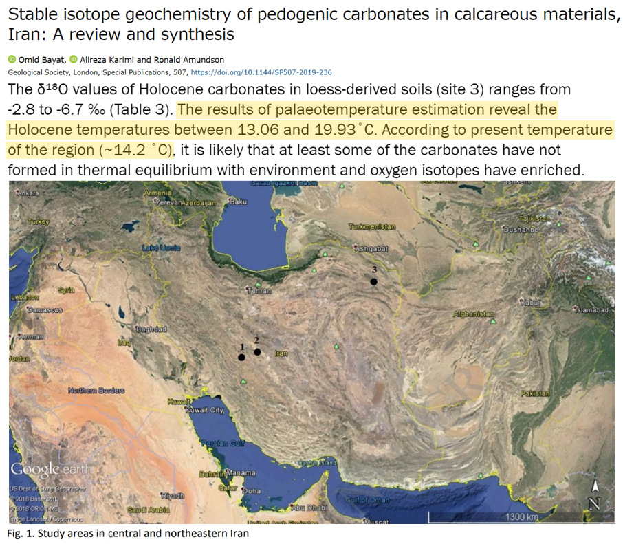
Bayat et al., 2020 Iran peak warming 5.73°C higher than present (19.93 vs. 14.2°C)
Application of a regression model, yielded from data of Holocene carbonates in the soils of North America, for these carbonates show formation temperatures between 12.7 and 15.7 ˚C with a dominant around 15˚C (Table 3). These temperatures are close to present temperature of Shahrekord (~12.7 ˚C) to maximum 3 ˚C warmer than present temperatures. … The results of palaeotemperature estimation reveal the Holocene temperatures between 13.06 and 19.93 ˚C. According to present temperature of the region (~14.2 ˚C), it is likely that at least some of the carbonates have not formed in thermal equilibrium with environment and oxygen isotopes have enriched.
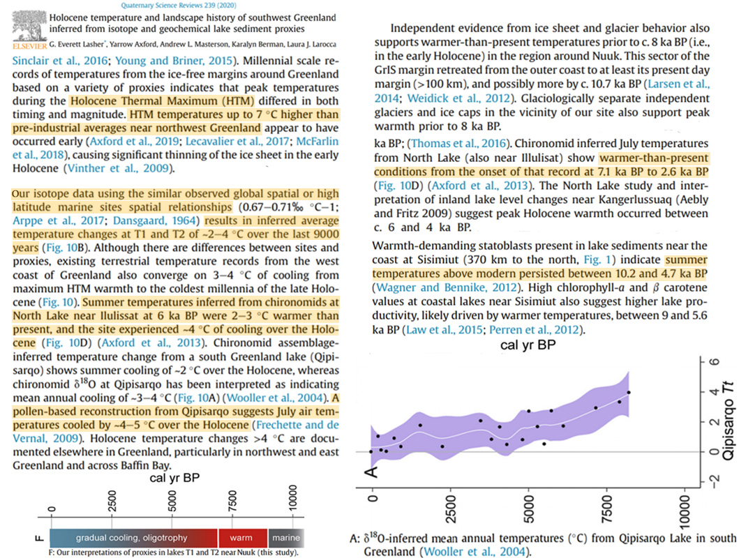
Lasher et al., 2020 NW Greenland temps “7°C higher than preindustrial”
[P]eak temperatures during the Holocene Thermal Maximum (HTM) differed in both timing and magnitude. HTM temperatures up to 7°C higher than pre-industrial averages near northwest Greenland appear to have occurred early (Axford et al., 2019; Lecavalier et al., 2017; McFarlin et al., 2018), causing significant thinning of the ice sheet in the early Holocene (Vinther et al., 2009).
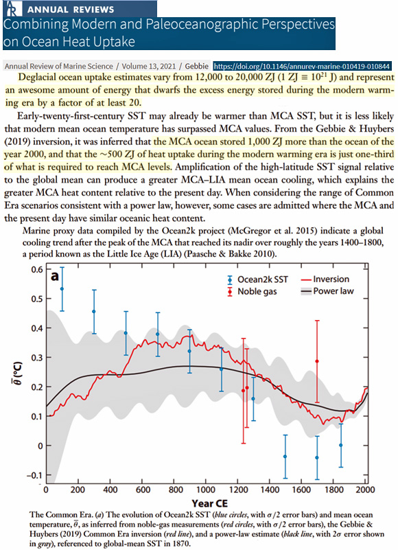
Gebbie, 2020 Modern global ocean heat 1/3rd of what’s required to reach Medieval levels
Ilyashuk et al., 2020 NW Germany ~3°C warmer 80,000 yrs ago (MIS 5a, glacial)
A subdivision of the MIS 5a interstadial into two very different climatic regimes is evident in the beetle (Coleoptera) record from Oerel, northwest Germany (Behre et al., 2005). Mild climate conditions with both summer (ca. 19 °C) and winter (2–4 °C) temperatures above present-day values (ca. 16 °C and ca. 1 °C for July and January, respectively) are recorded during the early part of the interstadial.
Găinuşă-Bogdan et al., 2020 Northern high latitudes “considerably warmer than today”
The mid-Holocene (MH: 6000 years Before Present) is a period for which reconstructions suggest a mean climate of the northern high latitudes that was considerably warmer than today in summer (Fischer et al. 2018), due to a different insolation forcing (Fig. 1). This is an interesting climate period, when the Sahara is suspected to have been greener than today (Claussen and Gayler 1997). … The mid-Holocene (6000 years before present) was a warmer period than today in summer in most of the Northern Hemisphere.
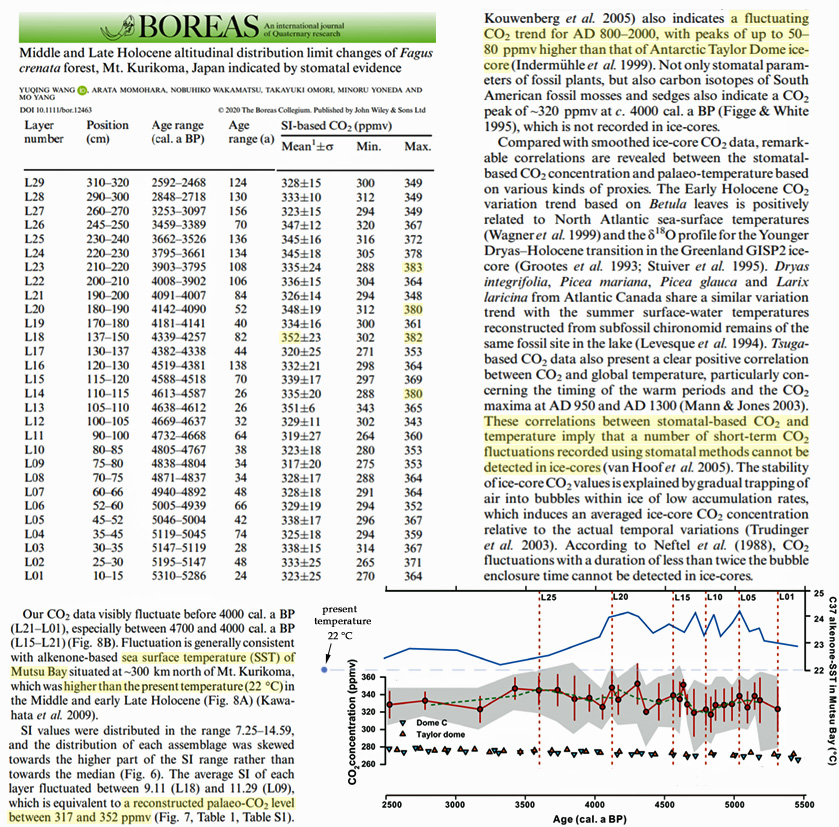
Wang et al., 2020 Japan temps warmer than present (22°C) for last 5500 years (CO2 ~280-380 ppm)
Results of palaeo-CO2 concentration reconstructed from the stomatal analysis indicate palaeo-CO2 fluctuation between 317 and 352 ppmv during the Middle–Late Holocene, which was more variable and higher than Greenland and Antarctic ice-core records … Fluctuation is generally consistent with alkenone-based sea surface temperature (SST) of Mutsu Bay situated at ~300 km north of Mt. Kurikoma, which was higher than the present temperature (22 °C) in the Middle and early Late Holocene.
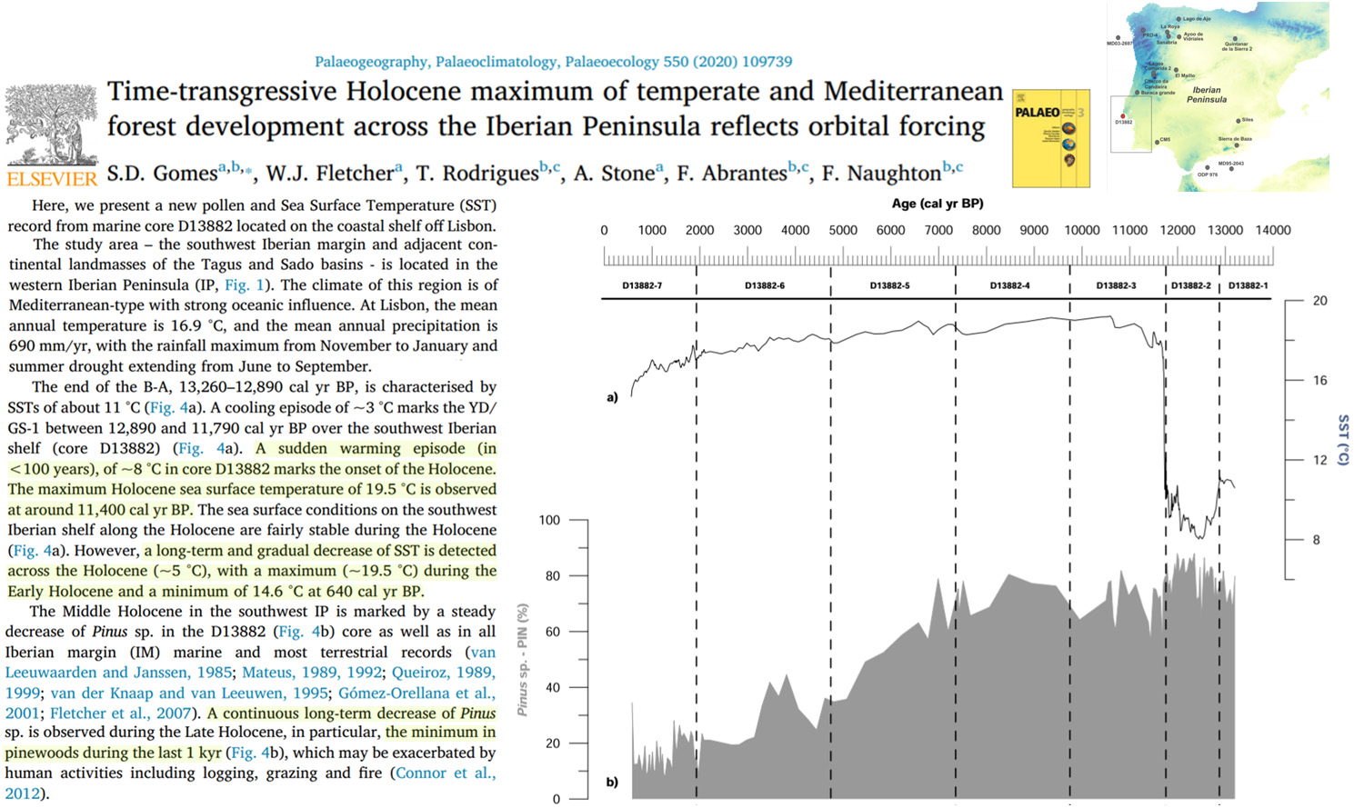
Gomes et al., 2020 Iberian SSTs 8°C warming in <100 years, Early Holocene 5°C warmer
A sudden warming episode (in <100 years), of ~8 °C in core D13882 marks the onset of the Holocene. The maximum Holocene sea surface temperature of 19.5 °C is observed at around 11,400 cal yr BP. The sea surface conditions on the southwest Iberian shelf along the Holocene are fairly stable during the Holocene (Fig. 4a). However, a long-term and gradual decrease of SST is detected across the Holocene (~5 °C), with a maximum (~19.5 °C) during the Early Holocene and a minimum of 14.6 °C at 640 cal yr BP.
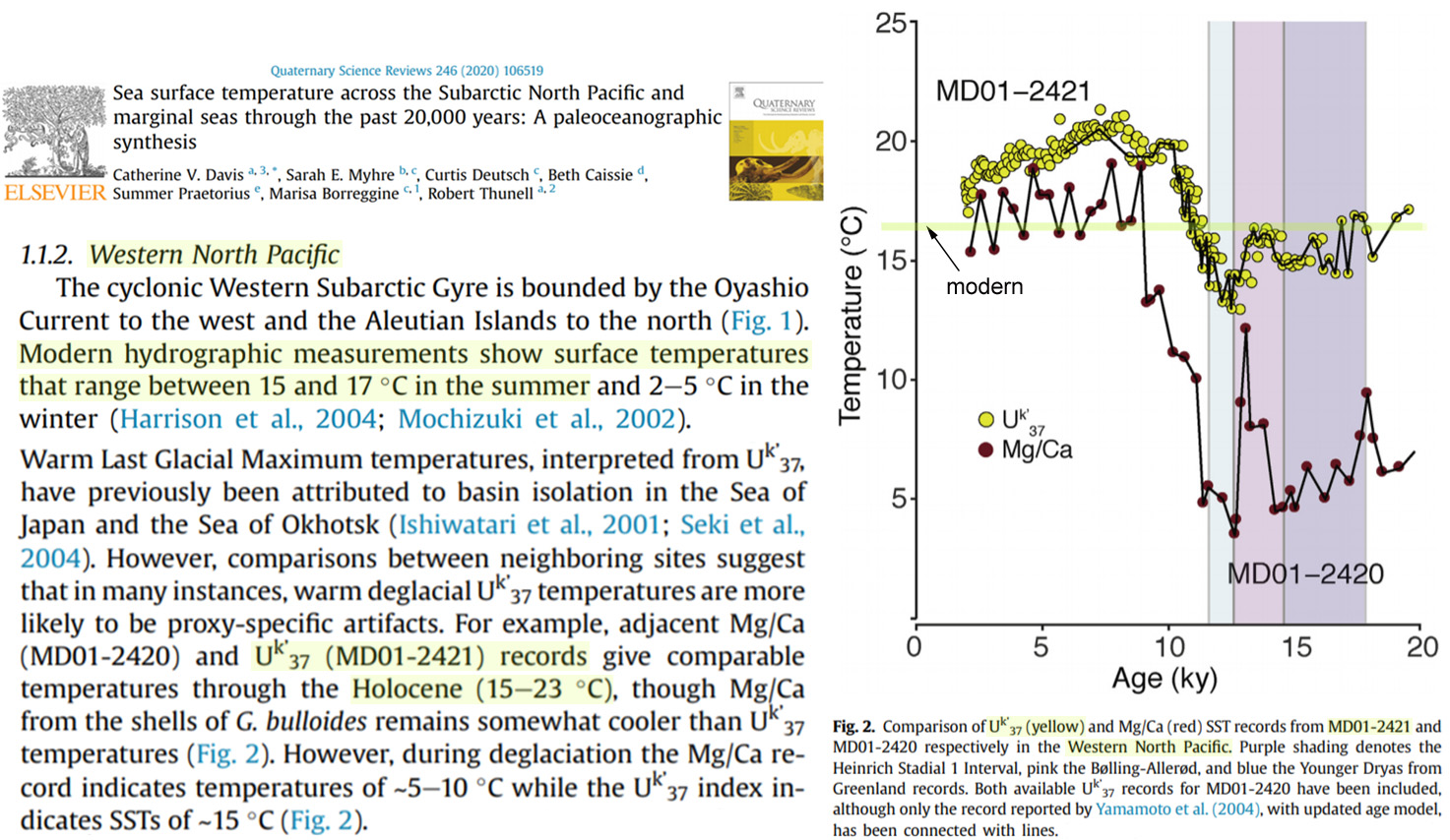
Davis et al., 2020 Western North Pacific peak SSTs up to 6°C warmer (23°C vs. 17°C)
Pearson et al., 2020 West Coast New Zealand SSTs “1.5 – 3°C warmer than today”
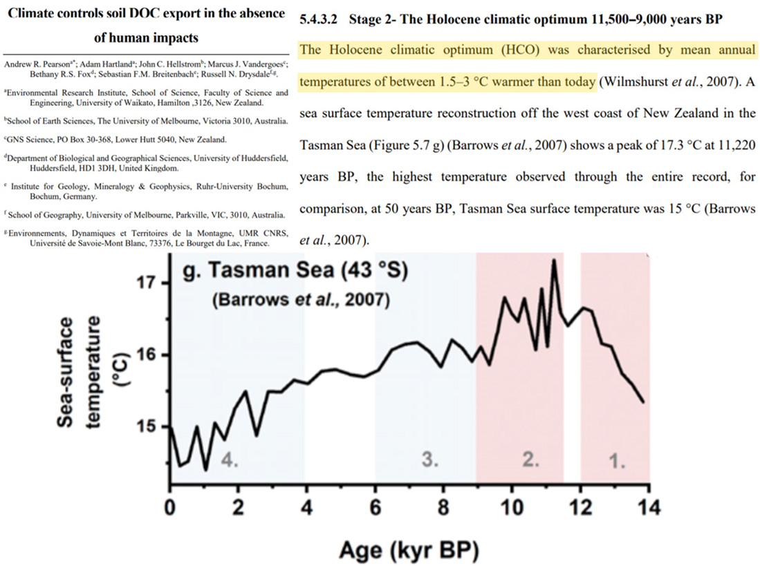
The Holocene climatic optimum (HCO) was characterised by mean annual temperatures of between 1.5–3 °C warmer than today (Wilmshurst et al., 2007). A sea surface temperature reconstruction off the west coast of New Zealand in the Tasman Sea (Figure 5.7 g) (Barrows et al., 2007) shows a peak of 17.3 °C at 11,220 years BP, the highest temperature observed through the entire record, for comparison, at 50 years BP, Tasman Sea surface temperature was 15 °C (Barrows et al., 2007).
Conti et al., 2020 Scotland lake summer temps 6.8°C warmer (~20°C vs. 13.2°C) 5600-5900 yrs ago
Notably, in this setting where the proxy should be most accurate, SSTs are remarkably similar to the present‐day average SST of Orkney, ranging from 7.1 °C in March to 13.2 °C in August, giving an average yearly temperature of 10.1 °C (https://www.seatemperature.org/europe/united-kingdom/orkney.htm). A proxy developed for freshwater lake sediments based on brGDGTs (Pearson et al., 2011; Table S4) was applied to the freshwater samples (from 197 to 118 cm). The results show a reconstructed summer lake temperature of 18.6–21.4 °C [~5939–5612 BP]. … The proxy‐calculated SST suggests a cooling trend towards values close to present‐day water temperatures at 77, 38 and 14 cm (13.1–10.5 °C, ± 4 °C).
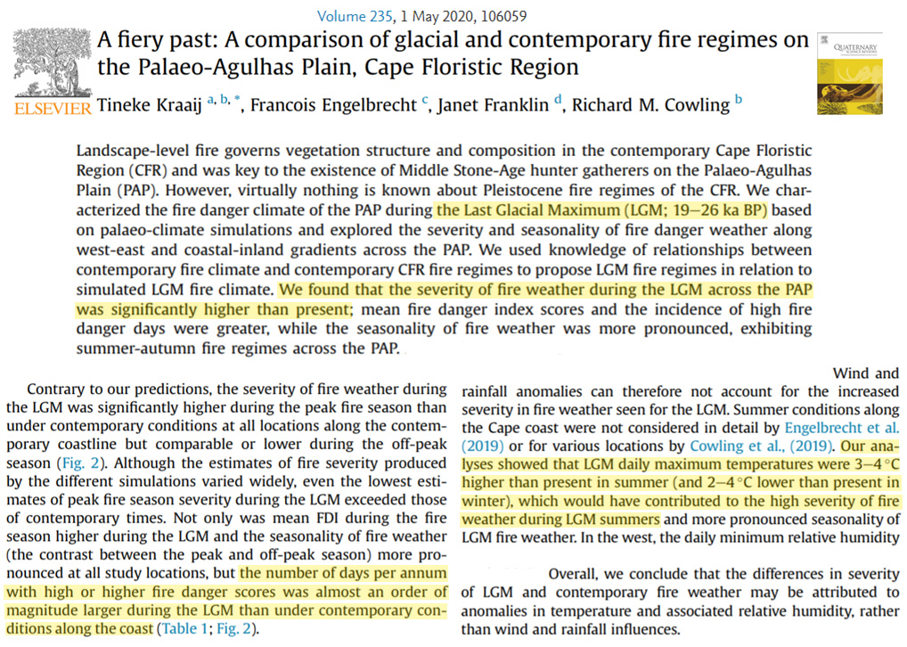
Kraaij et al., 2020 S. Africa “3-4°C higher than present in summer”, 10x more fire during last ice age (190 ppm CO2)
We found that the severity of fire weather during the LGM [last glacial maximum, 19-26 ka BP] across the PAP was significantly higher than present … [T]he number of days per annum with high or higher fire danger scores was almost an order of magnitude larger during the LGM [last glacial maximum, 19-26 ka BP] than under contemporary conditions along the coast … Our analyses showed that LGM [last glacial maximum, 19-26 ka BP] daily maximum temperatures were 3-4°C higher than present in summer (and 2-4°C lower than present in winter), which would have contributed to the high severity of fire weather during LGM summers.
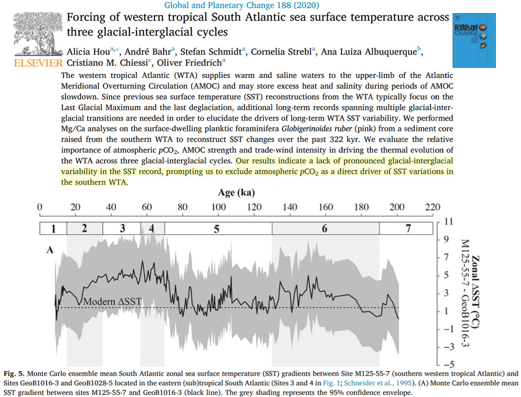
Hou et al., 2020 W. Tropical Atlantic 1-5°C warmer throughout last ice age (190 ppm CO2)
Our results indicate a lack of pronounced glacial-interglacial variability in the SST record, prompting us to exclude atmospheric pCO2 as a direct driver of SST variations in the southern WTA [western tropical Atlantic].
Schaney et al., 2020 Appalachian Mountains “considerably warmer than today” during the Mid Holocene
Eastern North America generally experienced a rise in temperature culminating with mid-Holocene Climatic Optimum, during which temperatures were considerably warmer than today (Beget, 1983; Driese et al., 2005; Fairbridge, 1982; Mullins et al., 2011; Springer et al., 2009; Wanner et al., 2015). The exact timing of the Climatic Optimum varied from region to region as did the coinciding abundance of available moisture (Barber et al., 1999; Clarke et al., 2003; Shuman and Marsicek, 2016; Viau et al., 2006; Zhao et al., 2010).
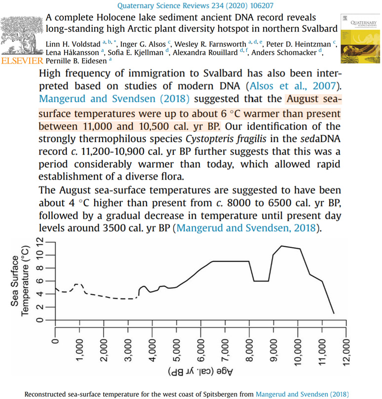
Voldstad et al., 2020 Svalbard (Arctic) 4-6°C warmer than today 9000-65000 yrs ago
The majority of paleoecological and geological records indicates that the Early-Mid Holocene period in Svalbard was warmer than today (c. 9000-5000 years ago; Hyvarinen, 1970; Birks, 1991; Birks et al., 1994; Salvigsen and Høgvard, 2006; Miller et al., 2010; Alsos et al., 2016; Farnsworth, 2018). According to Mangerud and Svendsen (2018), the August sea-surface temperature was possibly as much as 6°C higher than today. Based on present-day distributions, clone sizes, and genetic patterns, it is assumed that the most thermophilous plants in Svalbard had a broader distribution during the Early Holocene (Alsos et al., 2002; Engelskjøn et al., 2003; Birkeland et al., 2017). … The August sea-surface temperatures are suggested to have been about 4°C higher than present from c. 8000 to 6500 cal. yr BP, followed by a gradual decrease in temperature until present day levels around 3500 cal. yr BP (Mangerud and Svendsen, 2018).
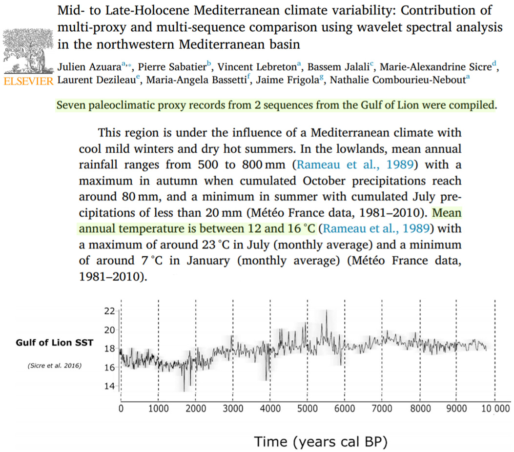
Azuara et al., 2020 Gulf of Lion SSTs mean annual temps 12-16°C (1981-2010), ~18°C Mid-Holocene
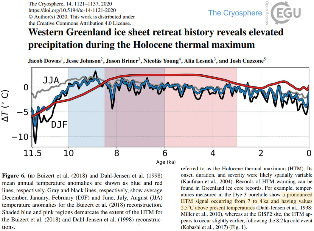
Downs et al., 2020 Greenland 2.5°C warmer than present from 7000-4000 yrs ago
Records of HTM warming can be found in Greenland ice core records. For example, temperatures measured in the Dye-3 borehole show a pronounced HTM signal occurring from 7 to 4 ka and having values 2.5◦C above present temperatures (Dahl-Jensen et al., 1998; Miller et al., 2010).
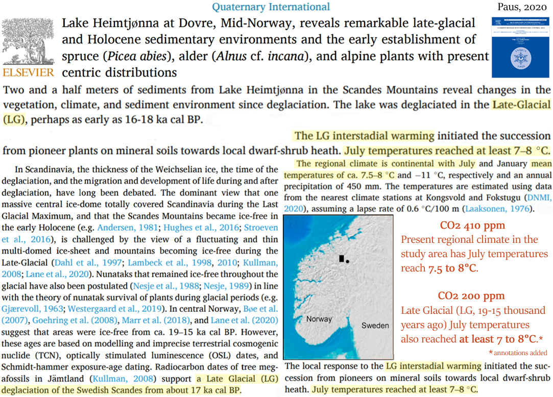
Paus, 2020 Scandes July temps today as cold as they were Late Glacial (CO2 190 ppm)
The regional climate is continental with July and January mean temperatures of ca. 7.5–8 ◦C and − 11 ◦C, respectively and an annual precipitation of 450 mm. … In LG [Late Glacial, 18 to 16 thousand years ago, CO2 ~200 ppm], July mean temperatures reached at least 7–8 ◦C locally (see 5.4.).
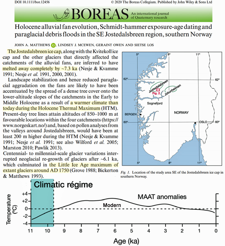
Matthews et al., 2020 Norway “warmer climate than today” smaller glaciers, higher tree lines
Landscape stabilization and hence reduced paraglacial aggradation on the fans are likely to have been accentuated by the spread of a dense tree cover onto the lower-altitude slopes of the catchments in the Early to Middle Holocene as a result of a warmer climate than today during the Holocene Thermal Maximum (HTM). Present-day tree lines attain altitudes of 850–1000 m at favourable locations within the four catchments (https://www.norgeskart.no/) and, based on pollen analyses from the valleys around Jostedalsbreen, would have been at least 200 m higher during the HTM (Nesje & Kvamme 1991; Nesje et al. 1991; see also Wilford et al. 2005; Marston 2010; Pawlik 2013). … The Jostedalsbreenice cap, along with theKvitekollice cap and the other glaciers that directly affected the catchments of the alluvial fans, are inferred to have melted away completely by ~7.3 ka (Nesje & Kvamme 1991; Nesje et al. 1991, 2000, 2001).
Hellstrom et al., 2020 New Zealand “at least 0.8–2.1 °C warmer”
The current upper surface altitude limit for flowstone growth seems likely to be in the 1000–1100 m range, which would require a minimum 100–200 m tree line altitude increase and at least 0.4–1.4 °C temperature increase for NB8 to grow during the Holocene optimum and earlier interglacials. Recently discovered passages linked to Nettlebed Cave include a section with flowstone beneath alpine terrain similar to that in Fig. 2 with a surface altitude of 1390 m asl, meaning it would have grown with a tree line at least 200–300 m higher than present under conditions at least 0.8–2.1 °C warmer. Reaching this site with drilling equipment will be a non-trivial task and the age of this growth event remains unknown for now.
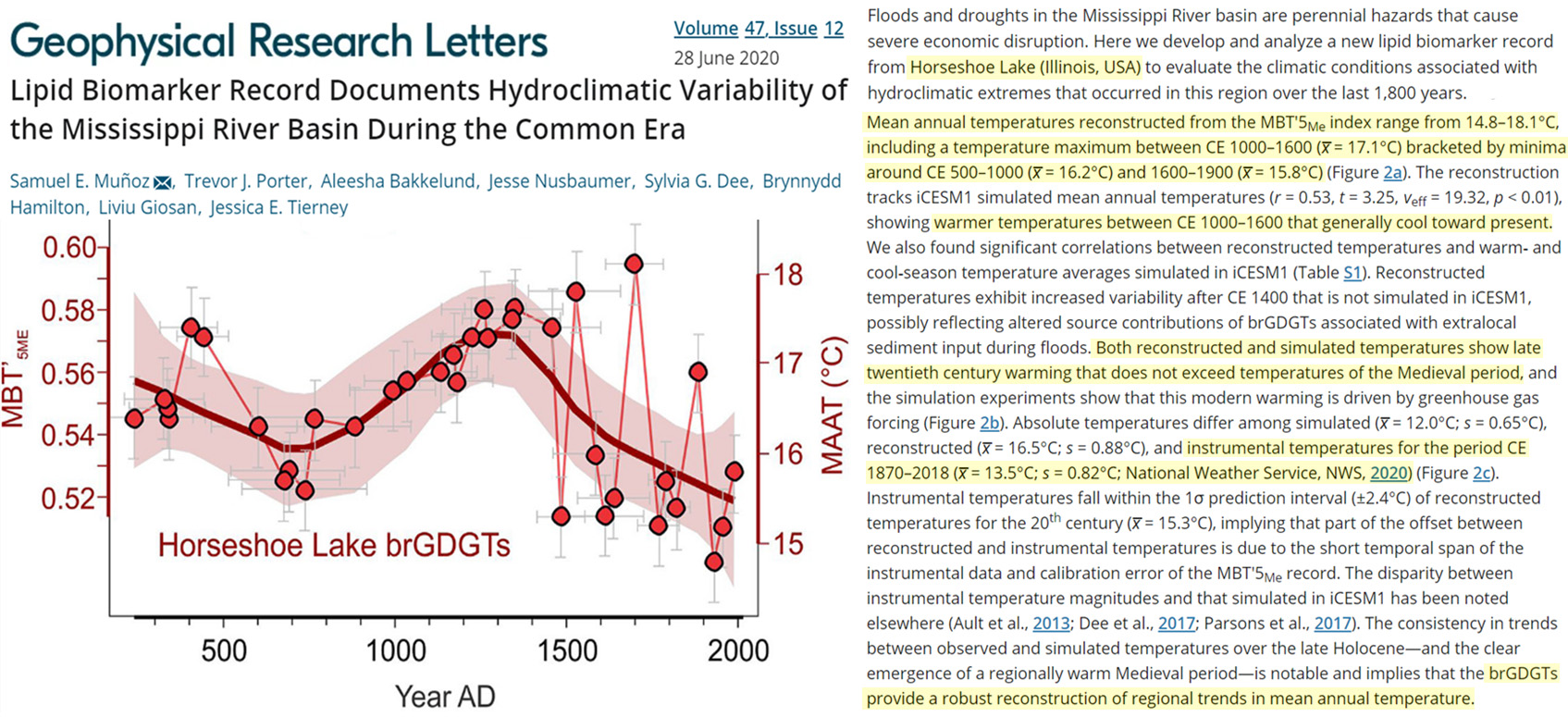
Muñoz et al., 2020 Illinois (USA) 13.5°C during 1870-2018, 17.1°C from CE 1000-1600
Mean annual temperatures reconstructed from the MBT’5Me index range from 14.8–18.1°C, including a temperature maximum between CE 1000–1600 (x̅ = 17.1°C) bracketed by minima around CE 500–1000 (x̅ = 16.2°C) and 1600–1900 (x̅ = 15.8°C) (Figure 2a). The reconstruction tracks iCESM1 simulated mean annual temperatures (r = 0.53, t = 3.25, νeff = 19.32, p < 0.01), showing warmer temperatures between CE 1000–1600 that generally cool toward present. … Both reconstructed and simulated temperatures show late twentieth century warming that does not exceed temperatures of the Medieval period … Absolute temperatures differ among simulated (x̅ = 12.0°C; s = 0.65°C), reconstructed (x̅ = 16.5°C; s = 0.88°C), and instrumental temperatures for the period CE 1870–2018 (x̅ = 13.5°C; s = 0.82°C; National Weather Service, NWS, 2020) (Figure 2c). Instrumental temperatures fall within the 1σ prediction interval (±2.4°C) of reconstructed temperatures for the 20th century (x̅ = 15.3°C).
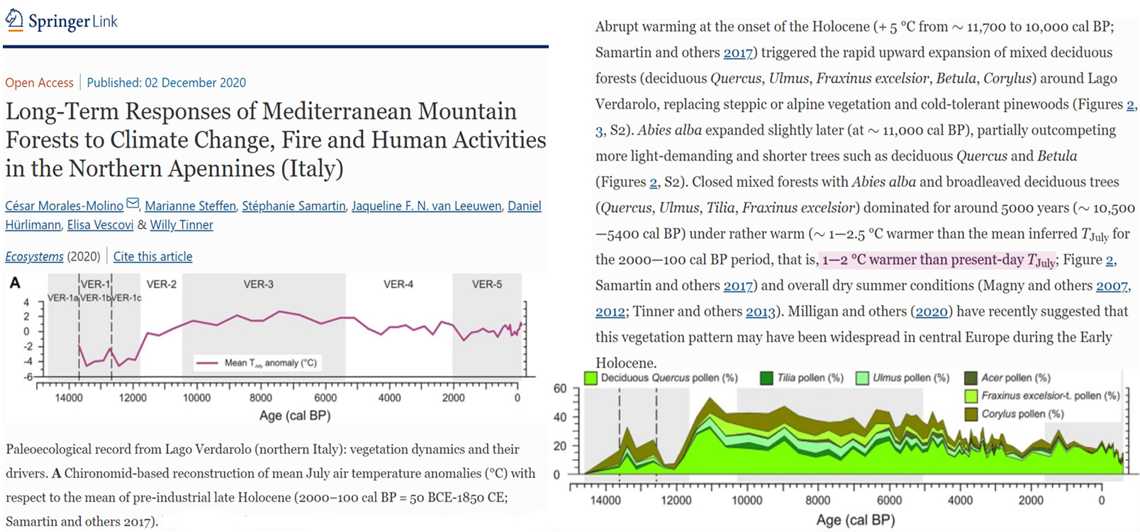
Morales-Molino et al., 2020 Mediterranean mountains 1-2°C warmer than today
“Species-rich mixed Abies alba (silver fir) forests dominated about 10,500—5500 years ago, under rather dry and warmer-than-today conditions (+ 1—2 °C).
Farnsworth et al., 2020 Iceland temperatures “2.5–3.2 °C greater than present”
Glaciers in Iceland exhibited their minimum extent sometime during the Holocene thermal maximum (HTM) between 7.9 and 5.5 ka BP (Striberger et al., 2012; Geirsdóttir et al., 2013). Synchronous with elevated northern hemisphere summer insolation, terrestrial and lacustrine proxy records suggest summer temperatures during this period were on the order of 2.5–3.2 °C greater than present (Caseldine et al., 2006; Harning et al., 2020). Models project Holocene glaciers in Iceland were non-existent or greatly reduced through the Middle Holocene (Flowers et al., 2008; Anderson et al., 2019).
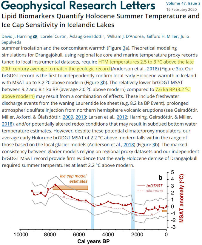
Harning eta l., 2020 Iceland “2.5 to 3 °C above the late 20th century average”
Theoretical modeling simulations for Drangajökull, using regional ice core and marine temperature proxy records tuned to local instrumental datasets, require HTM temperatures 2.5 to 3 °C above the late 20th century average to match the geologic record (Anderson et al., 2018) (Figure 3b). Our brGDGT record is the first to independently confirm local early Holocene warmth in Iceland with MSAT up to 3.2°C above modern (Figure 3b). The relatively lower brGDGT MSAT between 9.2 and 8.1 ka BP (average 2.0 °C above modern) compared to 7.6 ka BP (3.2 °C above modern) may result from a combination of effects. These include freshwater discharge events from the waning Laurentide ice sheet (e.g. 8.2 ka BP Event), prolonged atmospheric sulfate injection from northern hemisphere volcanic eruptions (see Geirsdóttir, Miller, Axford, & Ólafsdóttir, 2009, 2013; Larsen et al., 2012; Harning, Geirsdóttir, & Miller, 2018), and/or potentially altered redox conditions that may result in subdued bottom water temperature estimates. However, despite these potential climate/proxy modulators, our average early Holocene brGDGT MSAT of 2.2 °C above modern falls within the range of those based on the local glacier models (Anderson et al., 2018) (Figure 3b). The marked consistency between glacier models relying on regional proxy datasets and our independent brGDGT MSAT record provide firm evidence that the early Holocene demise of Drangajökull required summer temperatures at least 2.2 °C above modern.
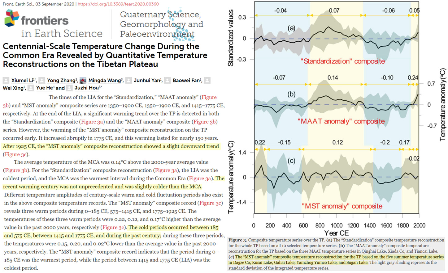
Li et al., 2020 Tibetan Plateau “recent warming…not unprecedented and…slightly colder than [Medieval]”
The average temperature of the MCA was 0.14°C above the 2000-year average value (Figure 3b). For the “Standardization” composite reconstruction (Figure 3a), the LIA was the coldest period, and the MCA was the warmest interval during the Common Era (Figure 3a). The recent warming century was not unprecedented and was slightly colder than the MCA. … The “MST anomaly” composite record (Figure 3c) reveals three warm periods during 0–185 CE, 575–1415 CE, and 1775–1925 CE. The temperatures of these three warm periods were 0.22, 0.12, and 0.17°C higher than the average value in the past 2000 years, respectively (Figure 3c). The cold periods occurred between 185 and 575 CE, between 1415 and 1775 CE, and during the past century.
Liu et al., 2020 Northern Asia “~2-3°C warmer than today”
During the Holocene Megathermal (8000-3000 cal yr BP), the climate of Northern Asia was a Holocene thermal and humidity maximum by other proxy data (Stebich et al., 2015), with summer temperatures ~2–3℃ warmer than today (Blinnikov et al., 2002; Valiranta et al., 2006). … In addition, the phytolith records suggests a significant climatic change from cool and dry conditions to warm and humid conditions during ~1600~300 cal yr BP, corresponding to the Medieval Warm Period (~1600~900 cal yr BP). Similarly, during ~1500~1100 cal yr BP, thermophilous Quercus, Juglans and Ulmus expanded obviously in the northwest Liaoning region (Zhang et al., 2004).
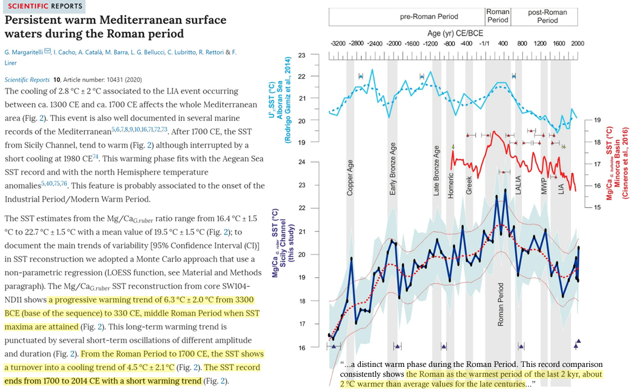
Margaritelli et al., 2020 Mediterranean Sea “about 2°C warmer” during the Roman Warm Period
This record comparison consistently shows the Roman as the warmest period of the last 2 kyr, about 2 °C warmer than average values for the late centuries for the Sicily and Western Mediterranean regions. After the Roman Period a general cooling trend developed in the region with several minor oscillations.
Elmslie et al., 2020 N. Ontario “~2-3°C warmer than the modern climate”
Modern Analog Technique (MAT) based on pollen was used to reconstruct average temperature over the Holocene record of Charland Lake and showed average temperature was ~2 °C warmer than present conditions ~7800–4500 cal yr BP, a time period which we define as the Holocene Thermal Maximum (HTM). … Atmosphere-ocean vegetation models have suggested that the HTM in northern Ontario was ~2–3 °C warmer than the modern climate (Renssen et al., 2009, 2012).
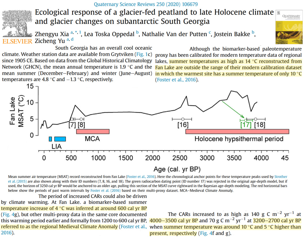
Xia et al., 2020 Subantarctic Georgia “summer temperature between 10°C and 5°C higher than present”
Although the biomarker-based paleotemperature proxy has been calibrated for modern temperature data of regional lakes, summer temperatures as high as 14°C reconstructed from Fan Lake are outside the range of their modern calibration dataset in which the warmest site has a summer temperature of only 10°C (Foster et al., 2016) … The CARs increased to as high as 140 g C m² yr¹ at 4000-3500 cal yr BP and 70 g C m² yr¹ at 3200-2700 cal yr BP when summer temperature was around 10°C and 5°C higher than present, respectively.
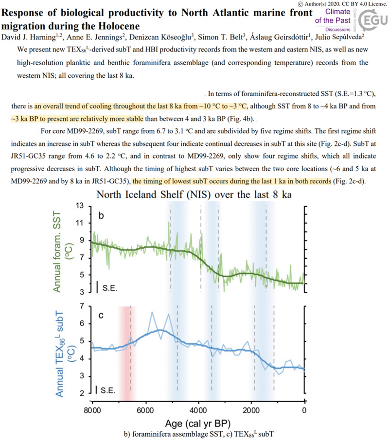
Harning et al., 2020 N. Iceland SSTs 7°C cooling trend (from ~10°C to ~3°C) last 8,000 yrs
In terms of foraminifera-reconstructed SST there is an overall trend of cooling throughout the last 8 ka from ~10 °C to ~3 °C, although SST from 8 to ~4 ka BP and from ~3 ka BP to present are relatively more stable than between 4 and 3 ka BP (Fig. 4b).

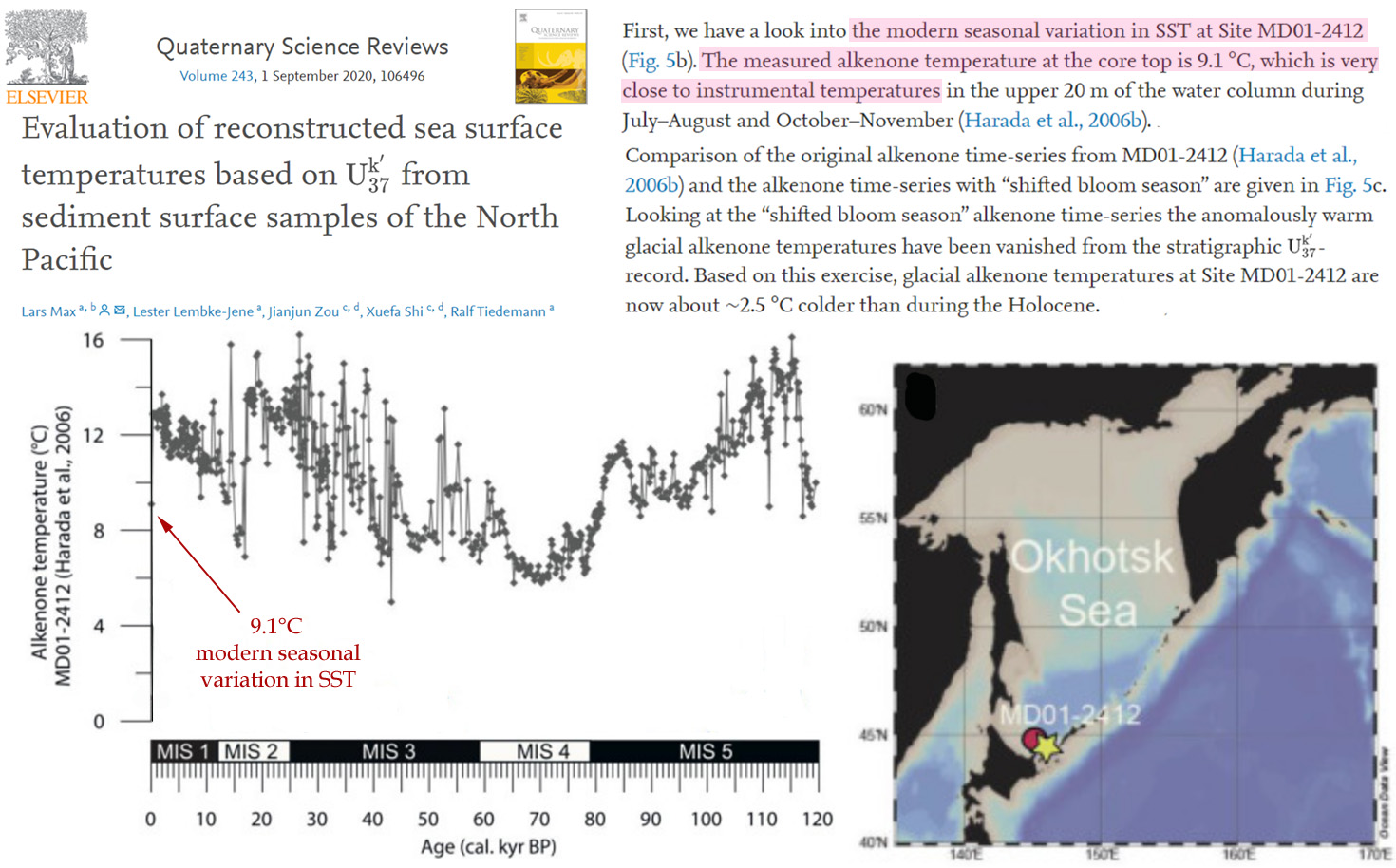
Max et al., 2020 N. Pacific SSTs ~14°C 20-25,000 yrs ago (glacial), 9.1°C today
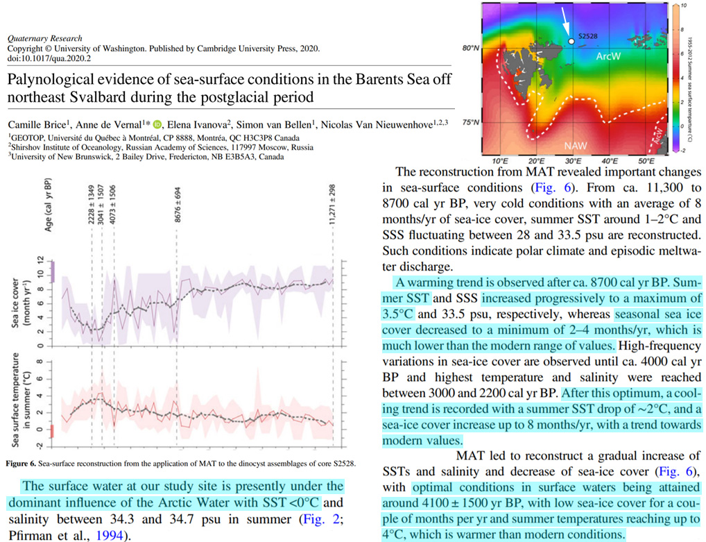
Brice et al., 2020 Svalbard <0°C today/11 mos. sea ice cover vs. 4°C/2 mos. sea ice cover ~4100 yrs ago
The surface water at our study site is presently under the dominant influence of the Arctic Water with SST <0°C and salinity between 34.3 and 34.7 psu in summer (Fig. 2; Pfirman et al., 1994). … The reconstruction from MAT revealed important changes in sea-surface conditions (Fig. 6). From ca. 11,300 to 8700 cal yr BP, very cold conditions with an average of 8 months/yr of sea-ice cover, summer SST around 1–2°C and SSS fluctuating between 28 and 33.5 psu are reconstructed. Such conditions indicate polar climate and episodic meltwater discharge. A warming trend is observed after ca. 8700 cal yr BP. Summer SST and SSS increased progressively to a maximum of 3.5°C and 33.5 psu, respectively, whereas seasonal sea ice cover decreased to a minimum of 2–4 months/yr, which is much lower than the modern range of values. … MAT led to reconstruct a gradual increase of SSTs and salinity and decrease of sea-ice cover (Fig. 6), with optimal conditions in surface waters being attained around 4100 ± 1500 yr BP, with low sea-ice cover for a couple of months per yr and summer temperatures reaching up to 4°C, which is warmer than modern conditions.
Birks, 2020 Denmark 2-3°C “warmer than today”
From fossil pollen occurrences, Iversen (1944) applied his modern climate envelopes (attributes) to infer that mid-Holocene summers were 2–3°C warmer and winters were 1–2°C warmer than today in Denmark. … Andersson proposed that mean July temperature in the early- and mid-Holocene was 2–2.5°C warmer than today.
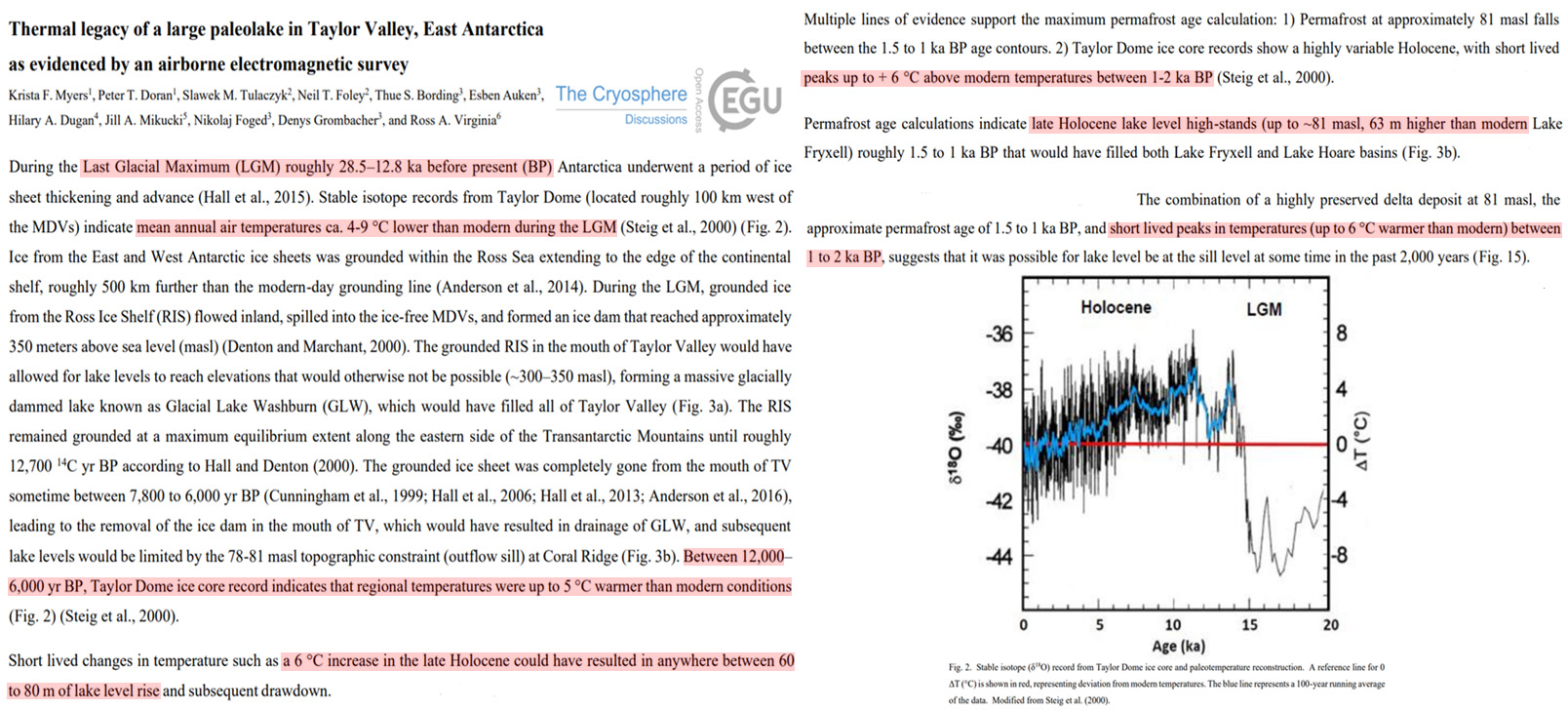
Myers et al., 2020 East Antarctica “6°C above modern temperatures” between 1-2 thousand yrs ago
Resistivity data suggests that active permafrost formation has been ongoing since the onset of lake drainage, and that as recently as 1,000 – 1,500 yr BP, lake levels were over 60 m higher than present. This coincides with a warmer than modern paleoclimate throughout the Holocene inferred by the nearby Taylor Dome ice core record. … Between 12,000–6,000 yr BP, Taylor Dome ice core record indicates that regional temperatures were up to 5 °C warmer than modern conditions (Fig. 2) (Steig et al., 2000). … Taylor Dome ice core records show a highly variable Holocene, with short lived peaks up to + 6 °C above modern temperatures between 1-2 ka BP (Steig et al., 2000). … Lake levels were higher potentially during and after the LGM when an ice dam blocked the mouth of TV, allowing for lake levels to increase by over 280 m compared to modern level. Taylor Dome ice core records indicate an abrupt warming of >15 °C from 15 – 12 ka BP, (Steig et al., 2000), which may have coincided with the maximum lake level of GLW.
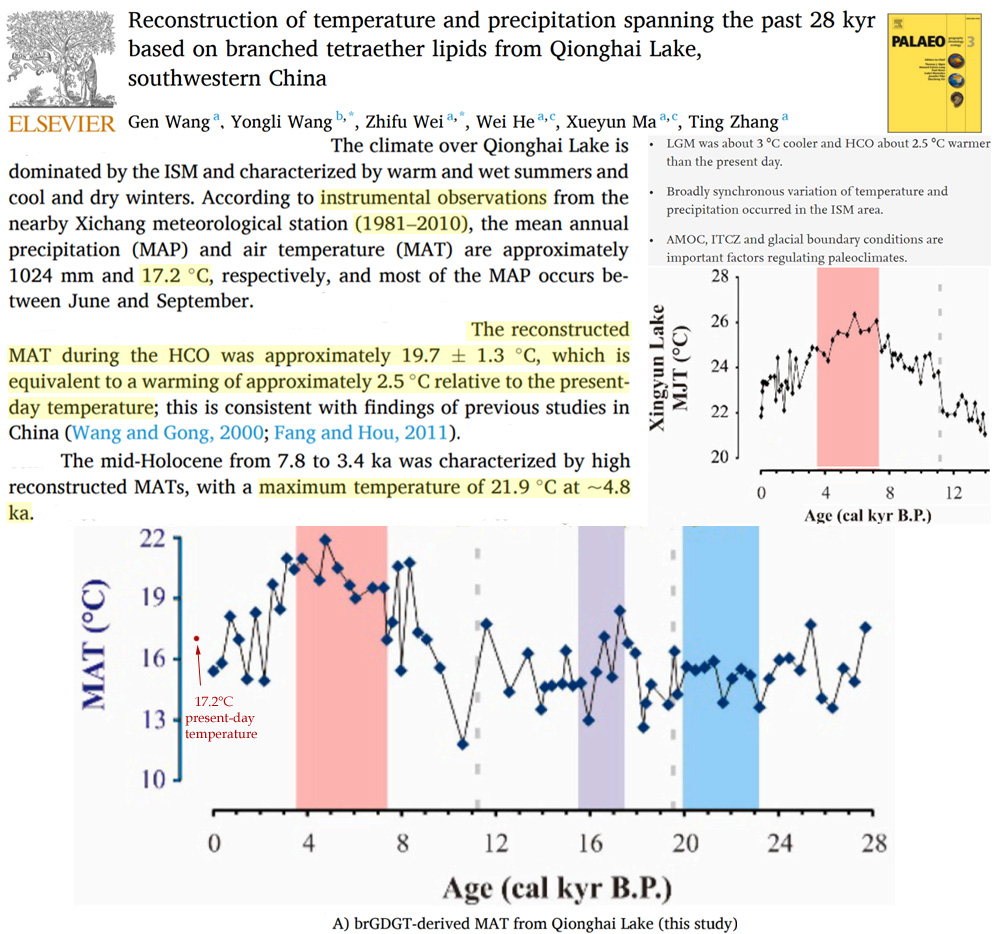
Wang et al., 2020 SW China “~2.5°C warmer than present-day”
We found that the temperature of the Last Glacial Maximum and Holocene Climatic Optimum was ~3 ◦C cooler and ~ 2.5 ◦C warmer than present-day conditions, respectively, based on brGDGTs-reconstructed mean annual air temperatures (MATs).
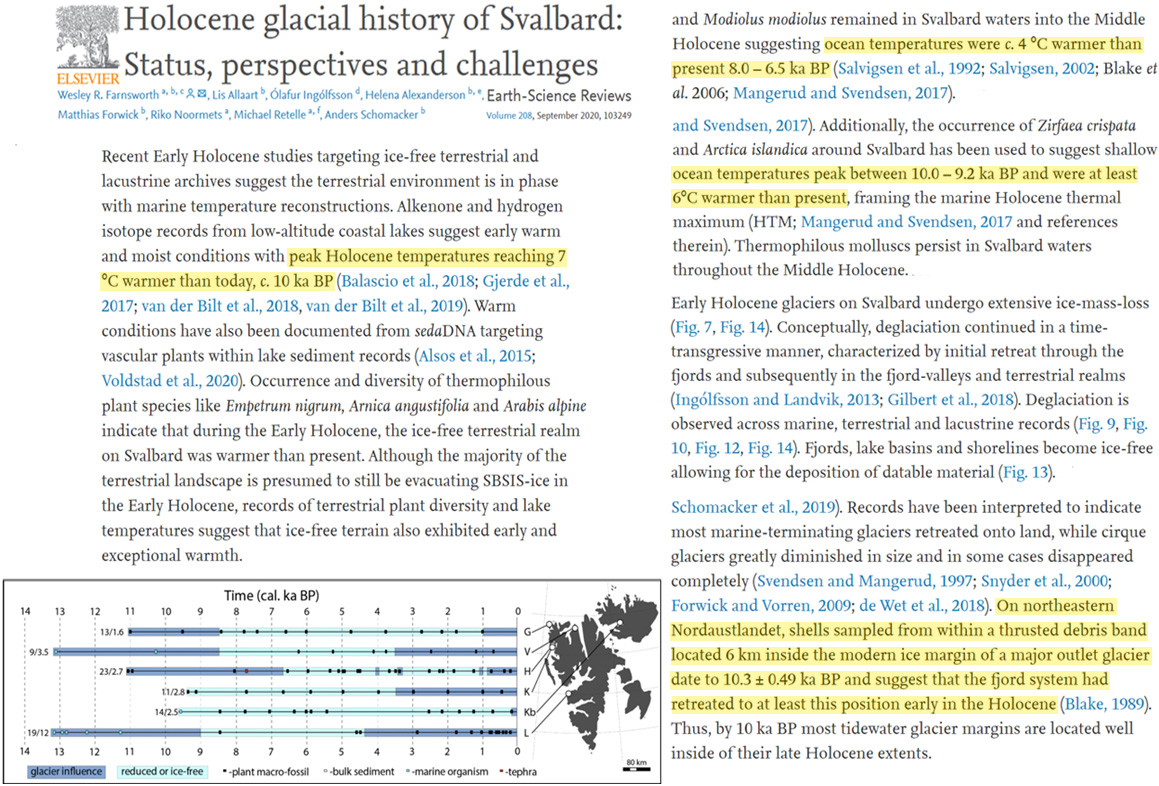
Farnsworth et al., 2020 Svalbard “7°C warmer than today” and ice free 10,000 yrs ago
Recent Early Holocene studies targeting ice-free terrestrial and lacustrine archives suggest the terrestrial environment is in phase with marine temperature reconstructions. Alkenone and hydrogen isotope records from low-altitude coastal lakes suggest early warm and moist conditions with peak Holocene temperatures reaching 7 °C warmer than today, c. 10 ka BP (Balascio et al., 2018; Gjerde et al., 2017; van der Bilt et al., 2018, van der Bilt et al., 2019). … [T]he occurrence of Zirfaea crispata and Arctica islandica around Svalbard has been used to suggest shallow ocean temperatures peak between 10.0 – 9.2 ka BP and were at least 6°C warmer than present, framing the marine Holocene thermal maximum (HTM; Mangerud and Svendsen, 2017 and references therein).
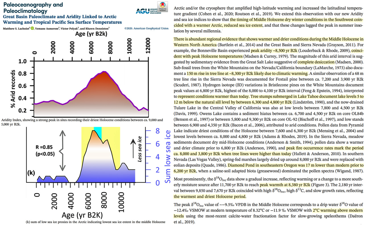
Lachniet et al., 2020 Western North America “2°C warming above modern levels, lowest sea ice extent”
The peak δ18Oivc value of ~−9.5‰ VPDB in the Middle Holocene corresponds to a drip water δ18O value of −12.4‰ VSMOW at modern temperature of 8.32°C or −11.9 ‰ VSMOW with 2°C warming above modern levels using the most‐recent calcite‐water fractionation factor for slow‐growing speleothems (Daëron et al., 2019). … Most prominently, the δ18Oivc data show a gradual increase, reflecting warming or a change to a more southerly moisture source after 11,700 yr B2k to reach peak warmth at 8,380 yr B2k (Figure 3). The 2,180 yr interval between 9,850 and 7,670 yr B2k coincided with high δ18Oivc, high δ13C, and slow growth rates, reflecting the warmest and driest Holocene period. … [T]he timing of Middle Holocene dry winter conditions in the Southwest coincided with a warmer Arctic, reduced sea ice extent.
Larocca et al., 2020 South Greenland at least 1.2-1.8°C warmer
Early Holocene summer temperatures in South Greenland were relatively cool and did not warm well beyond 1.2 °C above present. Peak warmth occurred in the mid-Holocene, between ∼7.1-5.5 ka BP, with summer temperatures at least 1.2–1.8 °C above present. Regrowth of local glaciers at ∼3.1, ∼1.3, and ∼1.2 ka BP reflect a broad, gradual pattern of cooling summer air temperatures. LIA historical moraines suggest summer air temperatures at least 0.4–0.9 °C cooler than present.
Kawahata et al., 2020 Japan “about 2°C higher than the present”
The alkenone SSTs around Funka Bay increased from 18.4℃ at 89AD, peaked at 23.2℃ in 759AD and decreased 17.4℃ at 1080AD. It is striking that the warm period overlaps with the prosperity of the Okhotsk culture in Hokkaido from the 5th to the 9th centuries, which corresponds to the most Hypsithermal period for the last 2000 years. … Based upon the topography with the distribution of shell middens, it is known that the lowland in Kanto of eastern Japan was flooded by seawater in 6.5-5.5 cal. kyr BP. This was the period when Corbicula japonica lived in brackish water more than 100 km away from the present-day shoreline and both corals and warm bivalves occurred at temperatures about 2°C higher than the present (Fig. 1a) (Matsushima, 2006). Tanabe et al. (2012) reconstructed detailed time-series sea level change in this area, where the sea level rose rapidly in the deglaciation period and slowly reached its highest in 7.4-4.5 cal. kyr BP by +4.0 m relative to the modern level (Tanabe et al., 2012).
Yao et al., 2020 Turpan (China) “0.5–1 °C warmer than at present” during the 9th century
The climate of the 9th–13th centuries in Turpan is recorded in historical documents. For example, Turpan experienced droughts in ad 840 and 843, consistent with the unusual warmth of Japan in the 9th century, and this period was 0.5–1 °C warmer than at present (Li 1985). Our quantitative estimation based on pollen data shows that the MAT in Turpan during the mid-9th–10th centuries was about 0.3 °C higher than today, while the annual precipitation was about 880 mm at that time (Table 4). In the 10th century, the climate changed from warm to cold, and became more humid. This lasted until the end of the 13th century. The temperature was 1 °C lower than the present value, and then gradually recovered until it was about 1 °C higher than today (Li 1985).
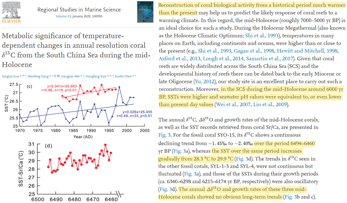
Guo et al., 2020 South China Sea ~2°C warmer with lower pH ~6000 yrs ago
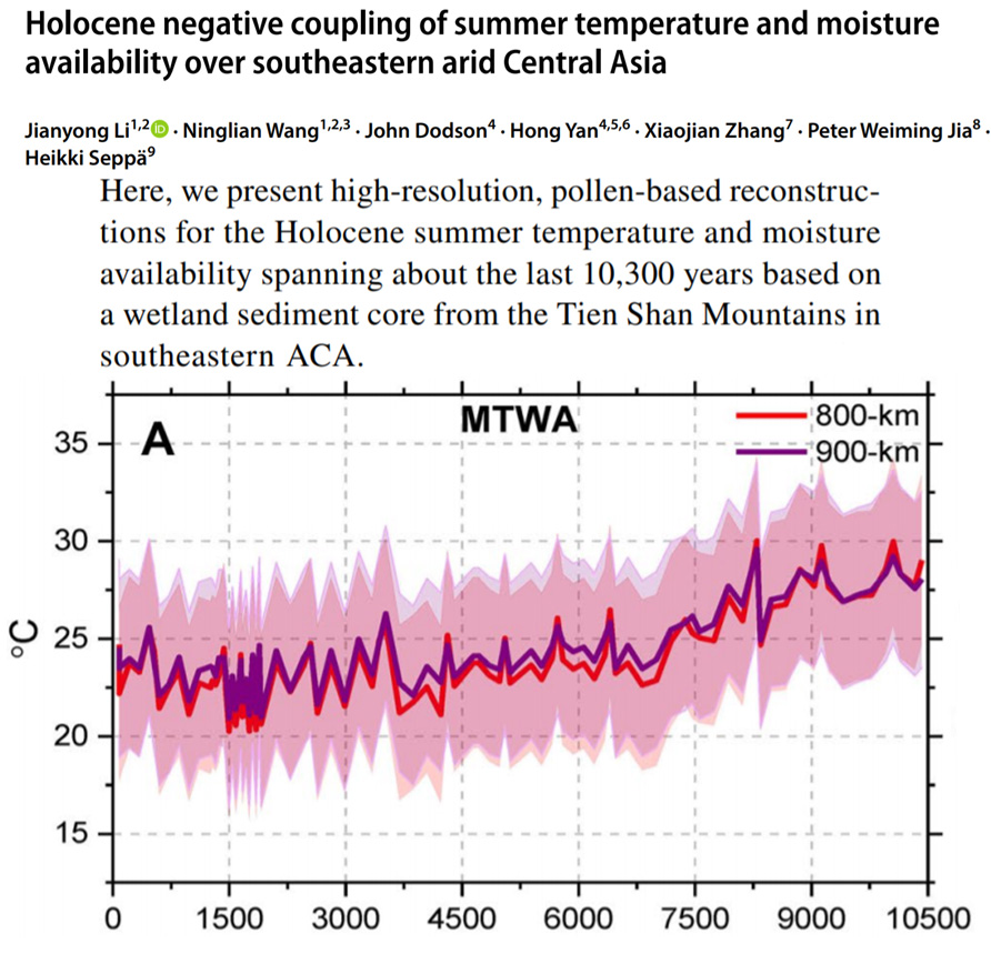
Li et al, 2020 Central Asia ~4-5°C warmer Early Holocene
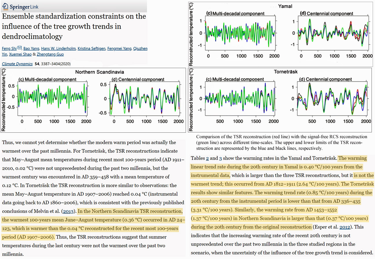
Shi et al., 2020 N. Scandinavia warmed 3.31°C/100 yrs from AD 336-435 vs. 0.85 °C/100 yrs 1901-2000
In the Northern Scandinavia TSR reconstruction, the warmest 100-years mean June–August temperature (0.36 °C) occurred in AD 24–123, which is warmer than the 0.04 °C reconstructed for the recent most 100-years period (AD 1907–2006). Thus, the TSR reconstructions suggest that summer temperatures during the last century were not the warmest over the past two millennia. … The warming linear trend rate during the 20th century in Yamal is 0.40 °C/100 years from the instrumental data, which is larger than the three TSR reconstructions, but it is not the warmest trend; this occurred from AD 1812–1911 (2.64 °C/100 years). The Torneträsk results show similar features. The warming trend rate (0.85 °C/100 years) during the 20th century from the instrumental period is lower than that from AD 336–435 (3.31 °C/100 years). Similarly, the warming rate from AD 1453–1552 (1.37 °C/100 years) in Northern Scandinavia is larger than that (0.37 °C/100 years) during the 20th century from the original reconstruction (Esper et al. 2012). This indicates that the increasing warming rate of the recent 20th century is not unprecedented over the past two millennia in the three studied regions in the scenario, when the uncertainty of the influence of the tree growth trend is considered.
Pilø et al., 2020 Melting ice in Norway reveal a warmer time during the Viking Age
Mountain passes have played a key role in past mobility, facilitating transhumance, intra-regional travel and long-distance exchange. Current global warming has revealed an example of such a pass at Lendbreen, Norway. Artefacts exposed by the melting ice indicate usage from c. AD 300–1500, with a peak in activity c. AD 1000 during the Viking Age—a time of increased mobility, political centralisation and growing trade and urbanisation in Northern Europe.
(press release) Melting Ice Has Revealed Artefacts From a Lost Viking Highway in Norway … As the Lendbreen ice patch recedes, it’s revealing an absolute treasure trove of artefacts, some of which have been buried under the ice for thousands of years. … After a careful study of these objects, archaeologists have now confirmed that the region was once a heavily trafficked mountain pass around a millennia ago – and not just a pass. The presence of horseshoes and other travel accoutrements indicates the region could have once been a bustling (for the time) Viking highway.
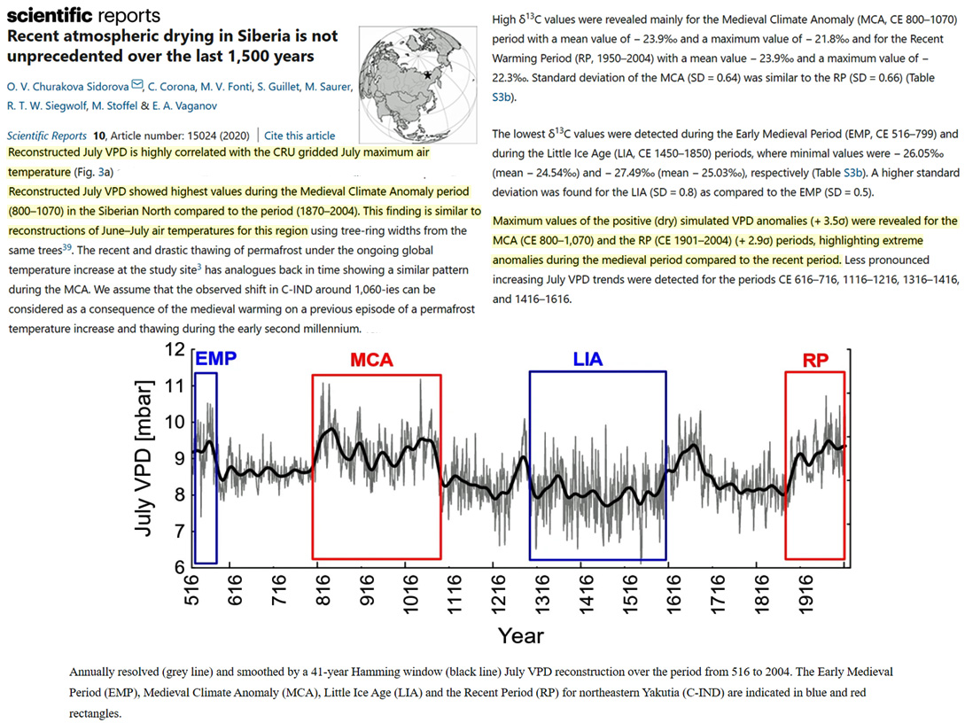
Churakova et al., 2020 Siberia “highest [VPD/temperature] values during the Medieval Climate Anomaly”
Reconstructed July VPD [vapor pressure deficit] is highly correlated with the CRU gridded July maximum air temperature … Maximum values of the positive (dry) simulated VPD anomalies (+ 3.5σ) were revealed for the MCA (CE 800–1,070) and the RP (CE 1901–2004) (+ 2.9σ) periods, highlighting extreme anomalies during the medieval period compared to the recent period. … Reconstructed July VPD showed highest values during the Medieval Climate Anomaly period (800–1070) in the Siberian North compared to the period (1870–2004). This finding is similar to reconstructions of June–July air temperatures for this region using tree-ring widths from the same trees.
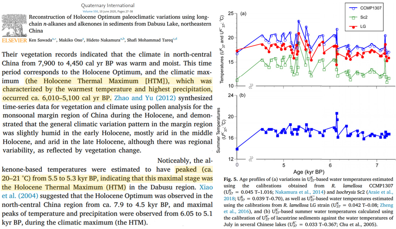
Sawada et al., 2020 NE China 3-5°C warmer during Holocene Thermal Maximum
Badgely et al., 2020 Greenland 1-2°C warmer than present
We focus on the last 20,000 years, which includes the end of the last glacial period, the glacial to interglacial transition, and the Holocene thermal maximum (HTM), when temperatures at the Greenland Ice Sheet summit reached 1-2 °C warmer than present (Cuffey and Clow, 1997; Dahl-Jensen et al., 1998).
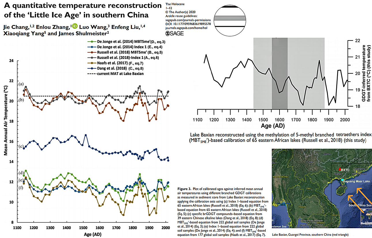
Chang et al., 2020 S. China warmer during Medieval times, 1400s, 1800s
Lesnek et al., 2020 SW Greenland “~2 °C above modern mean annual air temperature”
[N]umerical modeling indicates that warming of ~2 °C above modern mean annual air temperature is capable of producing sufficient melt to outpace mass gains from increased accumulation (Rae et al., 2012). This modest temperature increase is similar in magnitude to estimates of Arctic‐wide warming during the HTM (Kaufman et al., 2004). Therefore, our results suggest that in southwest Greenland, the warmest summer air temperatures over the entire Holocene occurred between ~10.4 and 9.1 ka.
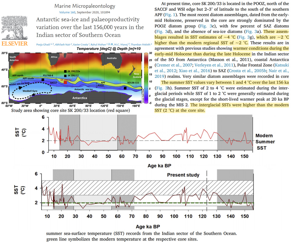
Ghadi et al., 2020 Southern Ocean site 2°C today, but 4°C 20,000 yrs ago and during the Early Holocene
At present time, core SK 200/33 is located in the POOZ, north of the SACCF and WSI edge but 2–3° of latitude to the south of the southern APF (Fig. 1). The most recent diatom assemblages, dated from the earlymid Holocene, preserved in the core are strongly dominated by the POOZ diatom group (Fig. 3c), with few percent of SAZ diatoms (Fig. 3d), and the absence of sea-ice diatoms (Fig. 3a). These assemblages resulted in SST estimates of ~4 °C, which are ~2 °C higher than the modern regional SST of ~2 °C. … Summer SST of 2 to 4 °C were estimated during the interglacial periods while SST of 1 to 2 °C were generally estimated during the glacial stages, except for the short-lived warmer peak at 20 ka BP during the MIS 2. The interglacial SSTs were higher than the modern SST (2 °C) at the core site.”
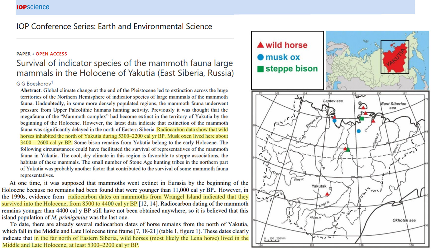
Boeskorov, 2020 Horses ate grass year-round along Arctic Ocean coast 5300-2200 yrs ago
Radiocarbon data show that wild horses inhabited the north of Yakutia during 5300–2200 cal yr BP. Musk oxen lived here about 3400 – 2600 cal yr BP. … To date, there are already several radiocarbon dates of horse remains from the north of Yakutia, which fall in the Middle and Late Holocene time frame. These dates clearly indicate that in the far north of Eastern Siberia, wild horses (most likely the Lena horse) lived in the Middle and Late Holocene, at least 5300–2200 cal yr BP.
Baumer et al., 2020 Laptev Sea (Arctic) “4°C warmer than today” Early Holocene
Pollen-based climate reconstructions from the Laptev Sea region inferred temperatures 4 °C warmer than today for the interval 11.5–8.4 cal. ka BP (Andreev et al. 2011), corresponding to the Holocene Thermal Maximum (HTM) at Lake Emanda at 11.5–9.0 cal. ka BP and at Lake El’gygytgyn at 11.4–7.6 cal. ka BP (Swann et al. 2010).
Hansen et al., 2020 Svalbard bottom waters 2°C warmer during last glacial/ice age
Hansen et al. (2017) speculated that the presence of the vesicomyids in the area, including similar old specimens at theGakkel Ridge in the Arctic Ocean, was made possible by the short-lived increase in bottom water temperature due to a subsurface current of northward advection of Atlantic water below the cold meltwater layer, which led to > 2°C warmer bottom water temperatures than in modern times (Rasmussen et al. 2007, 2014; Ezat et al. 2014, 2016; Sztybor & Rasmussen 2017a, b). … We documented a novel Arctic bivalve, Acharax svalbardensis sp. nov., present in sediment cores from active methane seeping pockmarks at Vestnesa Ridge off Svalbard, at 79N. The new species, Acharax svalbardensis sp. nov., co-occurred with recently described vesicomyids, dated to ~19,000–15,600 cal. years BP. This period of time corresponds to the Heinrich Stadial HS1, where surface water conditions were colder and bottom water conditions warmer (up to 2°C warmer) than today. We suggest that the presence of the newspecies and its restricted stratigraphical distribution are linked to the warmer bottom water conditions in the North Atlantic and Arctic region during HS1.
Orme et al., 2020 Southern Ocean SSTs “~1°C higher than today”
These data however suggest slightly 200 more extensive sea ice cover between 14 and 12 ka BP and after 8 ka BP, and a slight retreat of winter sea ice between 12.2 and 8 ka BP when SSTs were ~1°C higher than today. Relatively low values of the inferred winter sea ice concentration suggest only sporadic and relatively short-term (perhaps decadal to multidecadal scale) expansions of winter sea ice to the coring location throughout the Holocene.
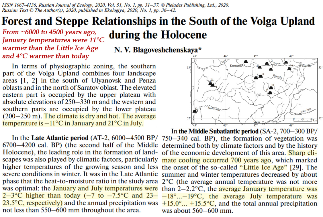
Blagoveshchenskaya, 2020 E. Europe winter temps 11°C warmer than Little Ice Age, 4°C warmer than today
In the Late Atlantic period (AT-2, 6000–4500 BP/6700–4200 cal. BP) (the second half of the Middle Holocene), the leading role in the formation of landscapes was also played by climatic factors, particularly higher temperatures of the growing season and less severe conditions in winter. It was in the Late Atlantic phase that the heat-to-moisture ratio in the study area was optimal: the January and July temperatures were 2–3°C higher than today (‒7 to –7.5°C and 23– 23.5°C, respectively) … Sharp climate cooling occurred 700 years ago, which marked the onset of the so-called “Little Ice Age” [29]. The summer and winter temperatures decreased by about 2°C (the average annual temperature was not more than 2–2.2°C, the average January temperature was –18°…–19°C, the average July temperature was +15.0°… +15.5°C.
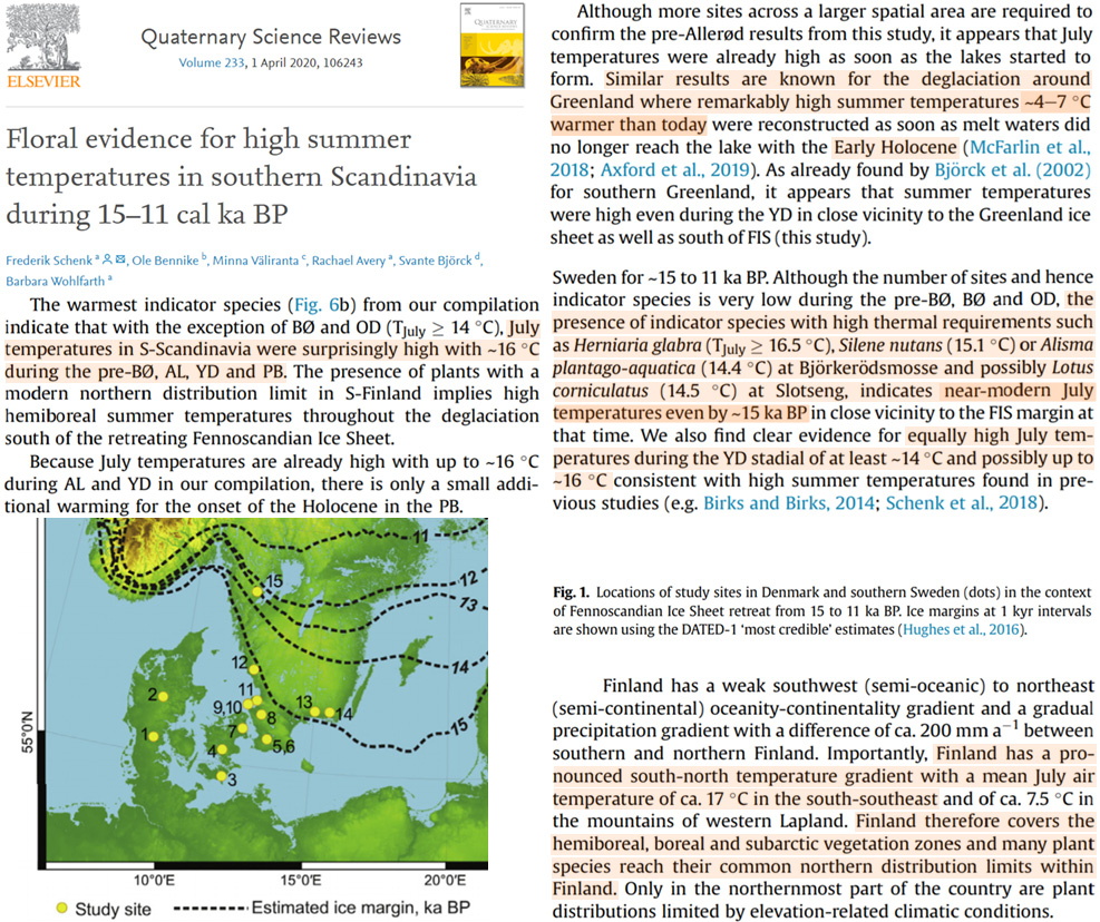
Schenk et al., 2020 Greenland temps 4-7°C warmer, Sweden temps already “near-modern” by 15,000 yrs ago
Although more sites across a larger spatial area are required to confirm the pre-Allerød results from this study, it appears that July temperatures were already high as soon as the lakes started to form. Similar results are known for the deglaciation around Greenland where remarkably high summer temperatures ~4-7°C warmer than today were reconstructed as soon as melt waters did no longer reach the lake with the Early Holocene (McFarlin et al., 2018; Axford et al., 2019). As already found by Bjorck et al. (2002) for southern Greenland, it appears that summer temperatures were high even during the YD in close vicinity to the Greenland ice sheet as well as south of FIS (this study). … Although the number of sites and hence indicator species is very low during the pre-BØ, BØ and OD, the presence of indicator species with high thermal requirements such as Herniaria glabra (TJuly ~16.5°C), Silene nutans (15.1°C) or Alisma plantago-aquatica (14.4°C) at Bjorker odsmosse and possibly Lotus corniculatus (14.5°C) at Slotseng, indicates near-modern July temperatures even by ~15 ka BP in close vicinity to the FIS margin at that time. We also find clear evidence for equally high July temperatures during the YD stadial of at least ~14°C and possibly up to ~16°C consistent with high summer temperatures found in previous studies (e.g. Birks and Birks, 2014; Schenk et al., 2018).
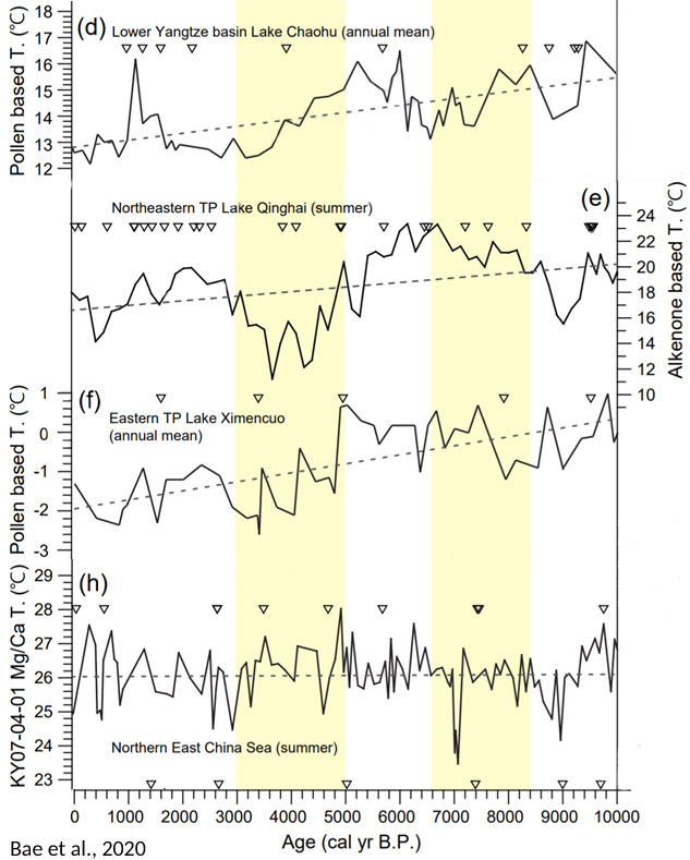
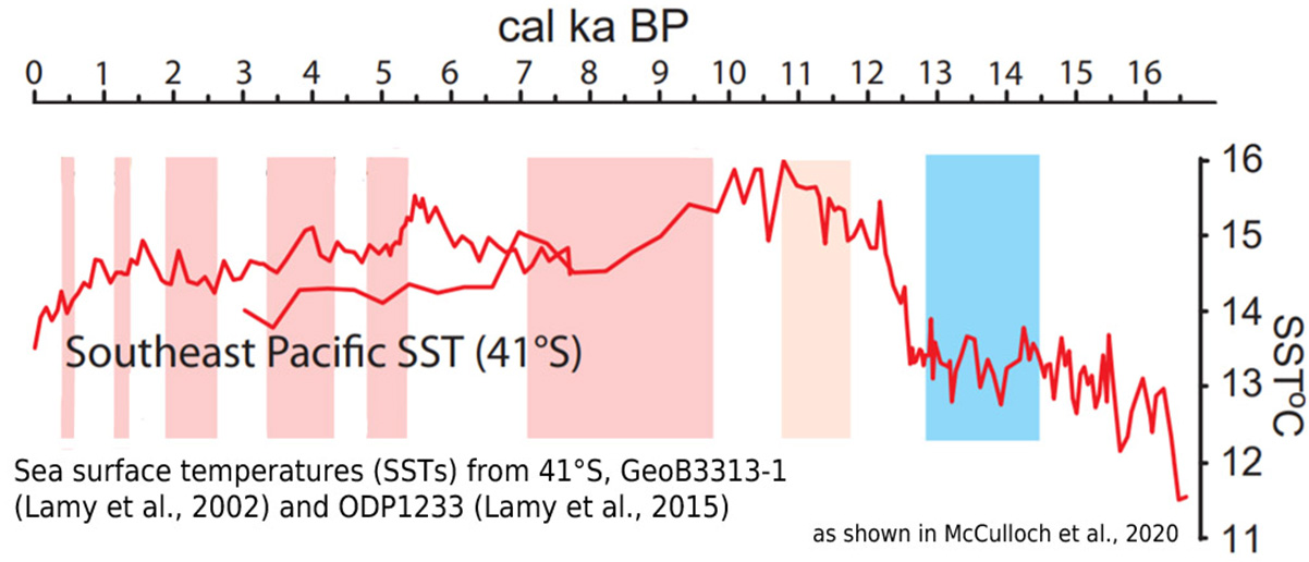
McCulloch et al., 2020 SE Pacific ~2°C warmer 11,000 yrs ago
Elmslie et al., 2020 “northern Ontario was ~2–3 °C warmer than the modern climate”
Atmosphere-ocean vegetation models have suggested that the HTM in northern Ontario was ~2–3 °C warmer than the modern climate (Renssen et al., 2009, 2012). Recent work from northwest Ontario (~1200 km to the west of our study site) reveals that the HTM occurred from ~8500–4500 cal yr BP (calendar years before present) and was ~2 °C warmer than present conditions. This estimate was calculated using a modern analog technique (MAT) calibration based on fossil pollen and a regional set of modern pollen and climate data (Moos and Cumming, 2011).
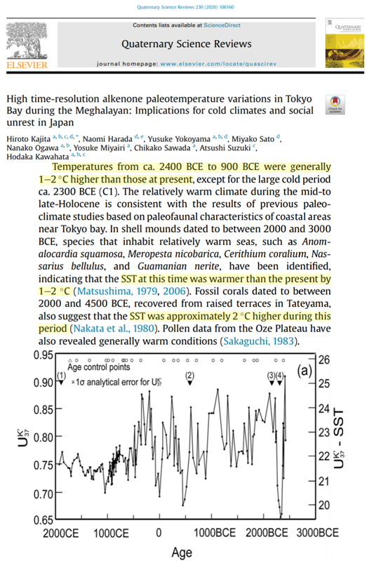
Kajita et al., 2020 Tokyo Bay temps 1-2°C higher than those at present
The reconstructed temperatures in Tokyo bay were generally higher than those in the present, exhibiting a declining trend over the long term, which roughly matches the changes in the orbitalforcing summer insolation throughout the northern hemisphere (Fig. 4a and b) (Laskar et al., 2004). This trend is also consistent with the millennial scale 2-3°C temperature decrease during the mid- to late-Holocene recorded in the core from the Boso peninsula … The timings of these cold periods were generally coincident with minimums in solar activity (Fig. 4c) and/or large volcanic eruptions, except for the coldest event, C1 (Fig. 4d) (Sigl et al., 2015; Solanki et al., 2004). … Temperatures from ca. 2400 BCE to 900 BCE were generally 1-2°C higher than those at present, except for the large cold period ca. 2300 BCE (C1). The relatively warm climate during the mid-to-late-Holocene is consistent with the results of previous paleoclimate studies based on paleofaunal characteristics of coastal areas near Tokyo bay. In shell mounds dated to between 2000 and 3000 BCE, species that inhabit relatively warm seas, such as Anomalocardia squamosa, Meropesta nicobarica, Cerithium coralium, Nassarius bellulus, and Guamanian nerite, have been identified, indicating that the SST at this time was warmer than the present by 1-2°C (Matsushima, 1979, 2006). Fossil corals dated to between 2000 and 4500 BCE, recovered from raised terraces in Tateyama, also suggest that the SST was approximately 2°C higher during this period (Nakata et al., 1980).
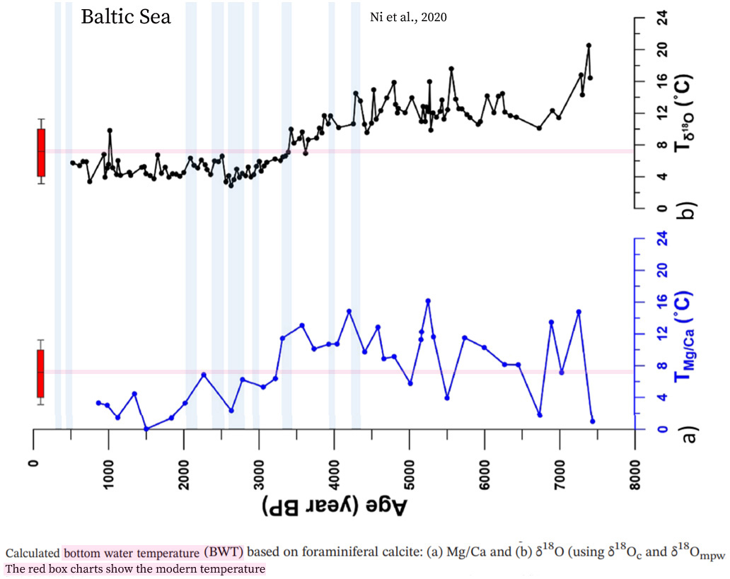
Ni et al., 2020 Holocene Baltic Sea bottom water temps peaked at 9-13°C warmer (16-20°C vs. 7°C)
Although the absolute temperature values of Mg/Ca‐based and δ18O‐based reconstructed bottom water temperature differ, both show a steady temperature decrease of ~7 °C from 4.1 to 2.5 ka BP. This coincides with the period of salinity decrease, indicating substantial environmental change. Tδ18O increased slightly around 2.5 ka BP, following the previous decrease, and became relatively less variable, with a mean Tδ18O value of 5.2 ± 1.2 °C. This is in the same range as modern bottom water temperature during winter or spring, which is known as the period when a majority of typical shallow‐water foraminiferal calcification occurs (e.g., Gustafsson & Nordberg, 2001). Mean temperature from both proxies was lowest between 2.5 and 0.5 ka BP (3.0 ± 2.1 °C). … During the beginning of Littorina Sea stage (~7.5–4.5 ka BP), the southern Baltic experienced multiple marine transgressions when the ongoing sea level rise outpaced glacioisostatic rebound (Björck et al., 2008). The mean sea level reached its highest level in the Baltic during the Littorina Sea stage (~7.5–~5 ka BP in Berglund et al., 2005). The water depth in the Little Belt increased considerably (~5–8 m) during these transgressions (Berglund et al., 2005), which led to a significant increase in North Sea water inflows due to deeper sills and straits.”
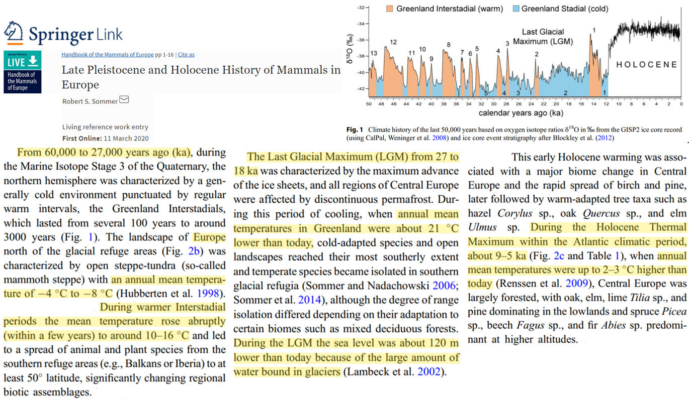
Sommer, 2020 Europe warmed -6°C to +13°C “within a few years” (interstadials); “2-3°C higher than today” 9-5 ka
From 60,000 to 27,000 years ago (ka), during the Marine Isotope Stage 3 of the Quaternary, the northern hemisphere was characterized by a generally cold environment punctuated by regular warm intervals, the Greenland Interstadials, which lasted from several 100 years to around 3000 years (Fig. 1). … The landscape of Europe north of the glacial refuge areas (Fig. 2b) was characterized by open steppe-tundra (so-called mammoth steppe) with an annual mean temperature of -4°C to -8° C (Hubberten et al. 1998)…. During warmer Interstadial periods the mean temperature rose abruptly (within a few years) to around 10–16°C and led to a spread of animal and plant species from the southern refuge areas (e.g., Balkans or Iberia) to at least 50 latitude, significantly changing regional biotic assemblages. … During the Holocene Thermal Maximum within the Atlantic climatic period, about 9–5 ka (Fig. 2c and Table 1), when annual mean temperatures were up to 2–3°C higher than today (Renssen et al. 2009), Central Europe was largely forested, with oak, elm, lime Tilia sp., and pine dominating in the lowlands and spruce Picea sp., beech Fagus sp., and fir Abies sp. predominant at higher altitudes.
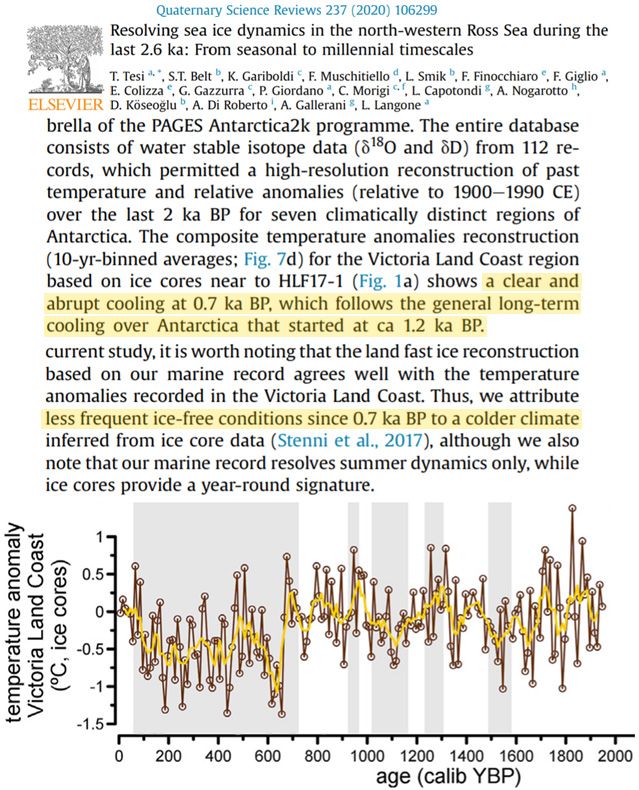
Tesi et al., 2020 Victoria Land, Antarctica, overall cooling last 700 years
Yao et al., 2020 West Central Asia warmer 1,000 yrs ago
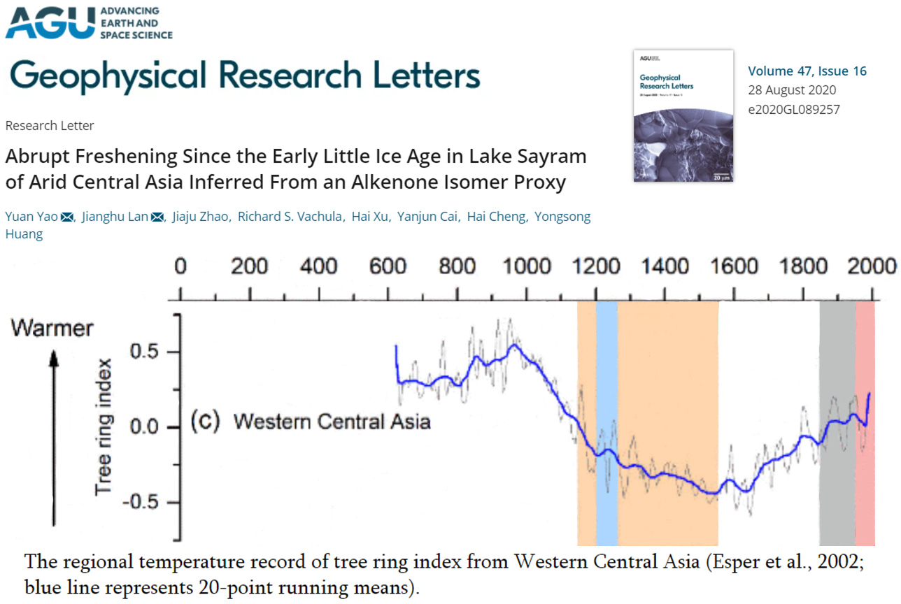
Fedorov et al., 2020 Arctic climate warmer 10-3,000 yrs ago, 4-8°C warmer last interglacial
In the recent past, Arctic climate was warmer than today at both the last interglacial (the Eemian, 130 to 110 thousand years ago; kyr) and the Holocene thermal maximum between 10 and 3 kyr (1, 5). Species distribution shifts, often associated with local extinction, were the most common response to the Late Quaternary environmental change (6). During warming events, Arctic tundra was reduced as boreal forest communities advanced to the north and was simultaneously restricted from northward retreat by the seacoast (1, 5). … Paleoclimate reconstructions show that the climatic optimum during the last interglacial was the warmest event of at least the past 250 kyr and this warmth strongly affected the Arctic biota (5). Terrestrial records suggest that the Arctic amplification produced last interglacial summer temperature anomalies 4 to 8 °C above present over the most of the Eurasian Arctic but a smaller increase of 2 to 4 °C was inferred in West Beringia (5). The last interglacial increase in summer temperature promoted the northward boreal forest expansion with tree line reaching the Arctic Ocean coastline and likely eliminating tundra from the landscape across the European (26, 27) and most of the Siberian Arctic (28, 29). … Notably, all modern cytochrome b sequences belong to the mtDNA lineage (EA5) that appeared in western Eurasia at 20.5 kyr (15), thus suggesting a recent origin for the phylogeographic structure revealed by our analysis of the present-day variation in nuclear and mitogenome. … Pollen and plant macrofossil records show that, over a large part of northern Eurasia, forest expanded to or near the Arctic coastline between 10 and 3 kyr during the Holocene thermal maximum (35–38).
McEwen et al., 2020 Norway temperatures “1.0 -3.0 °C higher than today”
Whereas the stabilization of the upper fan surface has been dated to within a millennium by exposure-age dating, the duration of the stable phase is very poorly constrained by the soil radiocarbon dates. Fan stability is likely to have persisted through a long interval of the mid Holocene when, from ~8.0 to 5. 5 ka, glaciers both in the neighbouring Smørstabbtindan massif and more widely throughout southern Norway were smaller than today and absent for much of the time (Matthews and Dresser, 2008; Nesje, 2009). This period of time corresponds with the Holocene Thermal Maximum (HTM) when, according to local and regional proxy records, mean annual air temperature is likely to have been 1.0 -3.0 °C higher than today (Dahl and Nesje, 1996; Jansen et al., 2008; Seppä et al., 2009; Velle et al., 2010; Lilleøren et al. 2012; Eldevik et al., 2014).
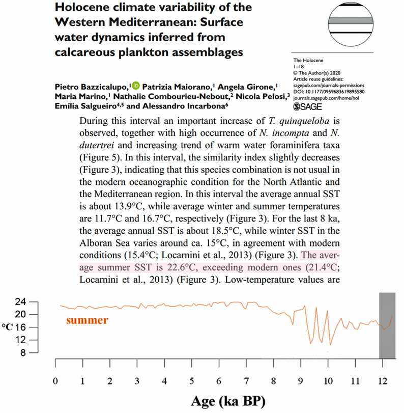
Bazzicalupo et al., 2020 Alboran Sea summer temperature 1.2°C warmer
For the last 8 ka, the average annual SST is about 18.5°C, while winter SST in the Alboran Sea varies around ca. 15°C, in agreement with modern conditions (15.4°C; Locarnini et al., 2013) (Figure 3). The average summer SST is 22.6°C, exceeding modern ones (21.4°C; Locarnini et al., 2013).
Lesnek et al., 2020 Greenland 2°C warmer 9-10,000 yrs ago
Model simulations suggest that the principal control on mass balance in land-based ice sheet areas in southwest Greenland is summer temperature (Cuzzone et al., 2019;Schlegel et al., 2016). Low levels of winter precipitation may also contribute to fast ice recession, and conversely, increased snowfall during periods of warmth has been hypothesized to partially offset temperature-driven mass loss (Thomas et al., 2016). However, numerical modeling indicates that warming of ~2 °C above modern mean annual air temperature is capable of producing sufficient melt to outpace mass gains from increased accumulation (Rae et al., 2012). This modest temperature increase is similar in magnitude to estimates of Arctic-wide warming during the HTM (Kaufman et al., 2004). Therefore, our results suggest that in southwest Greenland, the warmest summer air temperatures over the entire Holocene occurred between ~10.4 and 9.1 ka.
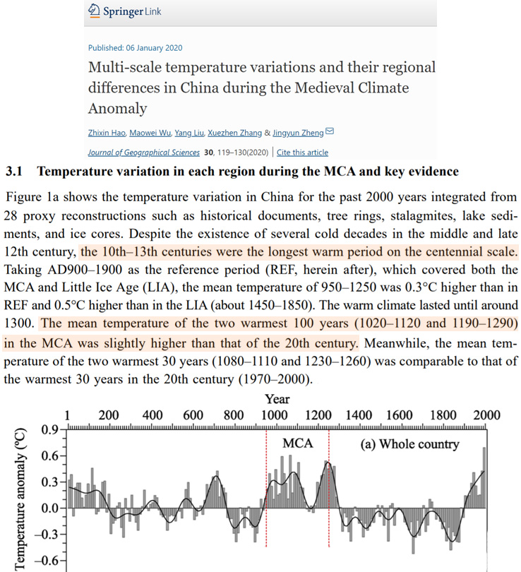
Hao et al., 2020 China warmer during Medieval Warm Period
Figure 1a shows the temperature variation in China for the past 2000 years integrated from 28 proxy reconstructions such as historical documents, tree rings, stalagmites, lake sediments, and ice cores. Despite the existence of several cold decades in the middle and late 12th century, the 10th–13th centuries were the longest warm period on the centennial scale. Taking AD900–1900 as the reference period (REF, herein after), which covered both the MCA and Little Ice Age (LIA), the mean temperature of 950–1250 was 0.3°C higher than in REF and 0.5°C higher than in the LIA (about 1450–1850). The warm climate lasted until around 1300. The mean temperature of the two warmest 100 years (1020–1120 and 1190–1290) in the MCA was slightly higher than that of the 20th century. Meanwhile, the mean temperature of the two warmest 30 years (1080–1110 and 1230–1260) was comparable to that of the warmest 30 years in the 20th century (1970–2000).
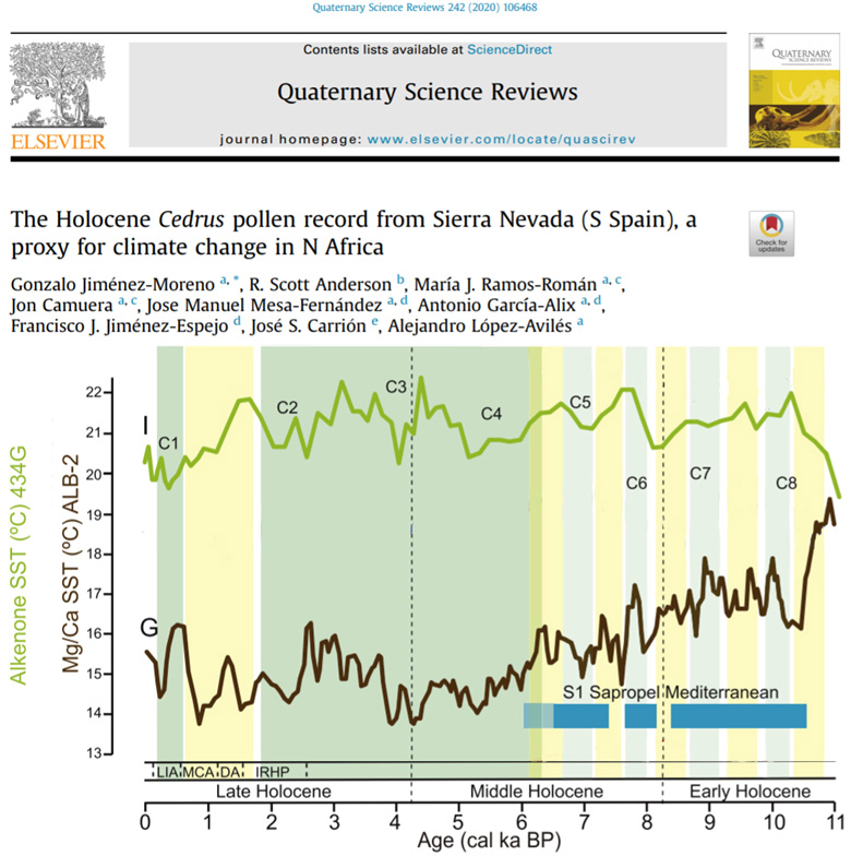
Jimenez-Moreno et al., 2020 Mediterranean SSTs 2-3°C warmer
Mikharevich et al., 2020 Western Siberia 1.5°C warmer during the Medieval Warm Period
However, the years of 850–870 and 930–950 AD were marked by summer cooling, and the years of 876–882 and 982 AD were marked by summer warming with average summer temperatures 1.5°C higher than the reference values of 1961–1990. The climatic variability of the Medieval period in different regions of the south of Western Siberia attests to the metachronous dynamics of the climate specified by the local conditions against the background of general climatic trends typical of Central Asia. … [I]n the 7th–18th centuries AD, the climate was somewhat warmer and wetter than at present. … In the period of 900–1000 AD, the mean annual temperature was 1–1.5°С higher, and precipitation was close to the modern one (according to palynological data).
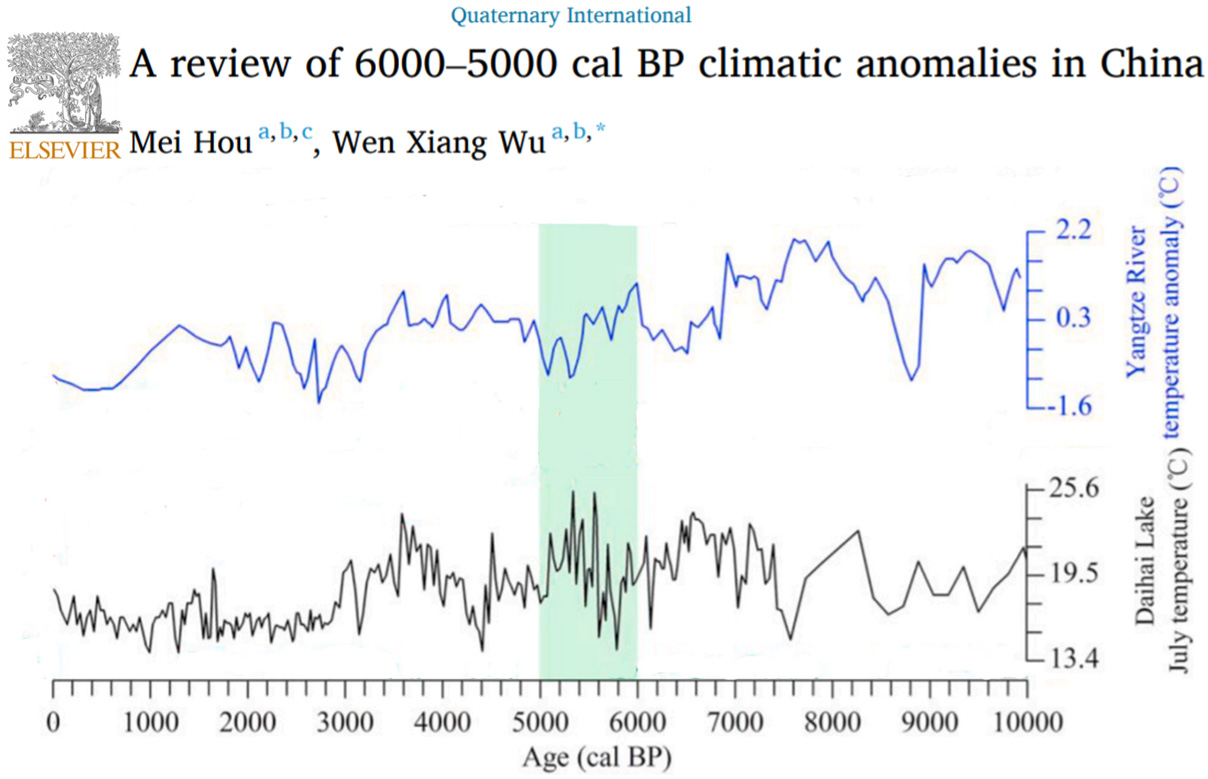
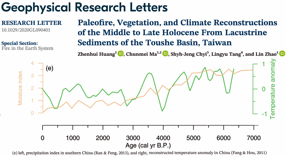
Hou and Wu, 2020 China, ~3°C warmer Early Holocene
Geoveta et al., 2020 Northern Iceland, 2-3°C warmer 5000-2500 yrs ago
The highest accumulation rate of the peat (Figure 4) is found between the tephra layers of Hekla 4 (4204 ± 52 cal yrs BP) and Hekla 3 (3000 ± 79 cal yrs BP). This period shows consistently higher levels of Betula pollen compared to the pre-Hekla 4 sample at c. 5000 BP. The higher levels of Betula suggest a warmer climate and is similar to the study of Einarsson (1968) that shows a period with drier and warmer conditions between 5000 and 2500 BP, where the annual mean temperatures were approximately 2–3°C higher than at present.
Huang et al., 2020 China as warm as today during Medieval Warm Period
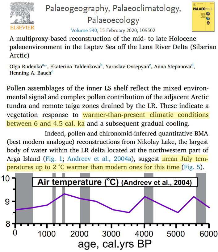
Rudenko et al., 2020 Siberian Arctic 2°C warmer
Pollen assemblages of the inner LS shelf reflect the mixed environmental signal and complex pollen contribution of the adjacent Arctic tundra and remote taiga zones drained by the LR. These indicate a vegetation response to warmer-than-present climatic conditions between 6 and 4.5 cal. ka and a subsequent gradual cooling … Indeed, pollen and chironomid-inferred quantitative BMA (best modern analogue) reconstructions from Nikolay Lake, the largest body of water within the LR delta located at the northwestern part of Arga Island, suggest mean July temperatures up to 2 °C warmer than modern ones for this time.
Goto-Azuma et al., 2020 East Greenland “2-3°C warmer than today”
Ongoing high-resolution analyses on the EGRIP core, the first deep ice core in East Greenland, will provide new insight into the mechanisms and impacts of environmental changes during the early Holocene, which was 2–3 ◦C warmer than today (Schüpbach et al., 2018).
Gavin et al., 2020 Eastern British Columbia “3.5°C warmer than today”
The early Holocene thermal optimum provides a good case of persistent, millennial-scale, increased seasonality and (potentially) increased drought (Shuman and Serravezza, 2017). Through the Holocene, decreasing summer insolation allowed expansion of moderated climate regimes and more mesic climates (Hebda, 1995). … While a detailed hydroclimate record does not exist near the site, Gerry Lake lithology and diatom assemblages suggests a shallow lake through the early Holocene (Westover, 2006) and a chironomid-inferred temperature reconstruction indicates summers were 3.5°C warmer than today (Chase et al., 2008).
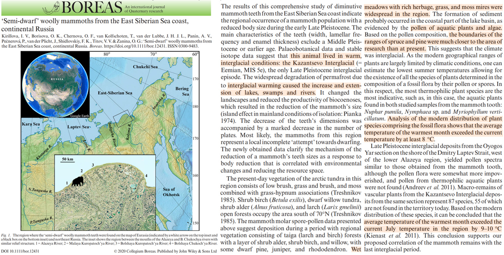
Kirillova et al., 2020 Siberian Arctic 9-10°C warmer last interglacial (280 ppm CO2)
Analysis of the modern distribution of plant species comprising the fossil flora shows that the average temperature of the warmest month exceeded the current temperature by at least 8 °C. … Macro-remains of vascular plants from the Kazantsevo Interglacial deposits from the same section represent 87 species, 55 of which are not found in the territory today. Based on the modern distribution of these species, it can be concluded that the average temperature of the warmest month exceeded the current July temperature in the region by 9–10 °C (Kienast et al. 2011). This conclusion supports our proposed correlation of the mammoth remains with the last interglacial period.
Recent Decades/Centuries Cooling/Non-Warming
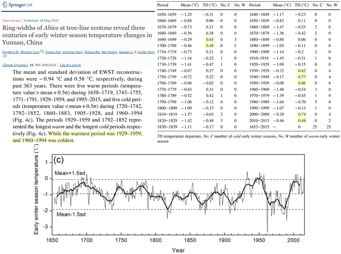
Yingfeng et al., 2020 SW China, 1960-1994 coldest of last 400 years, 2010-2015 same temps as 1700-1709
The mean and standard deviation of EWST reconstructions were − 0.94 °C and 0.58 °C, respectively, during past 363 years. There were five warm periods (temperature value>mean+0.5σ) during 1658–1719, 1743–1755, 1771–1791, 1929–1959, and 1995–2015, and five cold periods (temperature value<mean+0.5σ) during 1720–1742, 1792–1852, 1860–1883, 1905–1928, and 1960–1994. The periods 1929–1959 and 1792–1852 represented the longest warm and the longest cold periods respectively (Fig. 4c). While the warmest period was 1929–1959, and 1960–1994 was coldest.
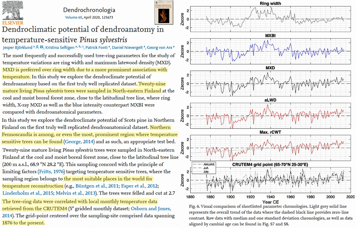
Björklund et al., 2020 Finland temps warmer than recent decades in the 1930-’40s
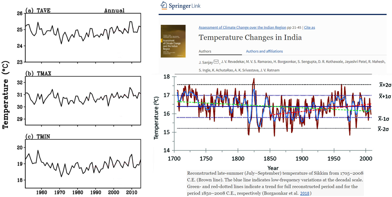
Sanjay et al., 2020 India warmer in the 1700s
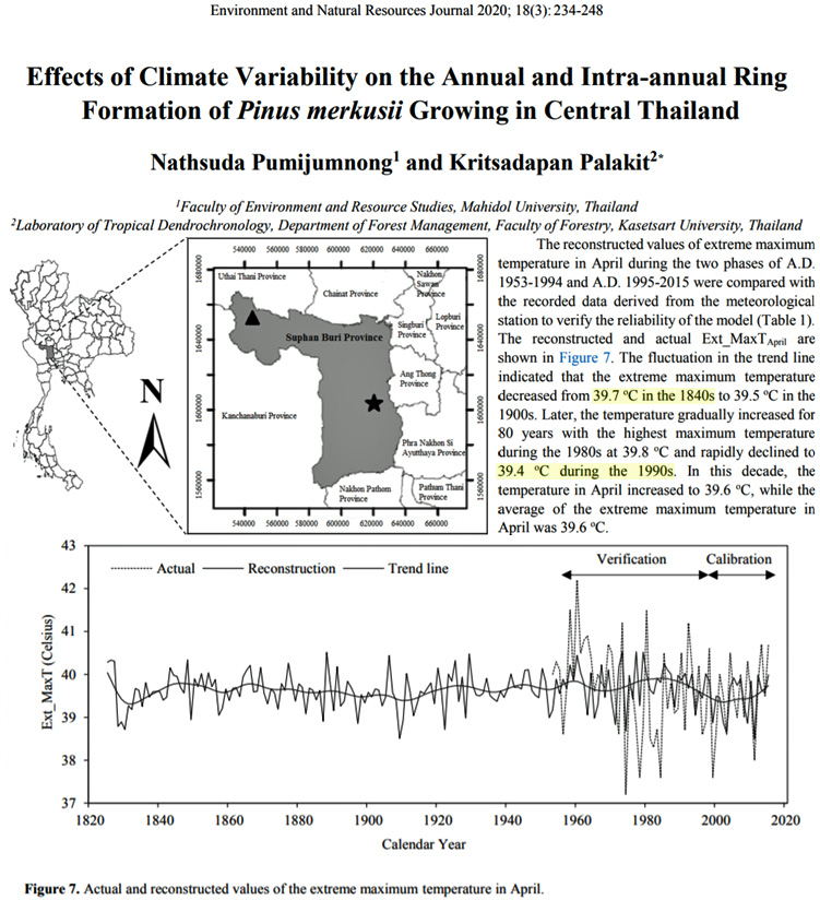
Pumijumnong and Palakit, 2020 Thailand warmer in the 1840s than 1990s
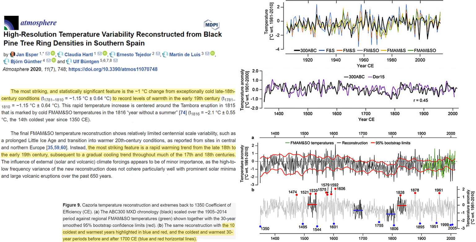
Esper et al., 2020 Spain warmer in 1600s, warmed 1°C from late 1700s to early 1800s
The most striking, and statistically significant feature is the ~1 °C change from exceptionally cold late-18th-century conditions to record levels of warmth in the early 19th century. This rapid temperature increase is centered around the Tambora eruption in 1815 that is marked by cold FMAM&SO temperatures in the 1816 “year without a summer” [74] (t1816 = −2.1 °C ± 0.55 °C, the 14th coldest year since 1350 CE).
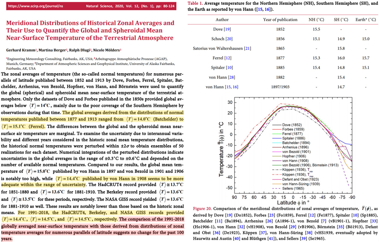
Kramm et al., 2020 Global temperature calculation the same today (14.5°C) as late 1800s
The results derived from the historical data suggest no change in the globally averaged near-surface temperature over the past 100 years.
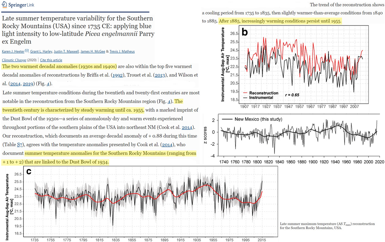
Heeter et al., 2020 Southern Rockies (USA) “After 1955, a cooling trend occurs for the next ca. 50 years”
The two warmest decadal anomalies (1930s and 1940s) are also within the top five warmest decadal anomalies of reconstructions by Briffa et al. (1992), Trouet et al. (2013), and Wilson et al. (2014, 2019) … Late summer temperature conditions during the twentieth and twenty-first centuries are most notable in the reconstruction from the Southern Rocky Mountains region (Fig. 4). The twentieth century is characterized by steady warming until ca. 1955, with a marked imprint of the Dust Bowl of the 1930s—a series of anomalously dry and warm events experienced throughout portions of the southern plains of the USA into northeast NM (Cook et al. 2014). Our reconstruction, which documents an average decadal anomaly of + 0.88 during this time (Table S7), agrees with the temperature anomalies presented by Cook et al. (2014), who document summer temperature anomalies for the Southern Rocky Mountains (ranging from + 1 to + 2) that are linked to the Dust Bowl of 1934. The period of prolonged warming in the 1930s through the 1950s is consistent with other reconstructions in other areas of North America (Briffa et al. 1992; Trouet et al. 2013; Wiles et al. 2019). … After 1955, a cooling trend occurs for the next ca. 50 years until 2000.
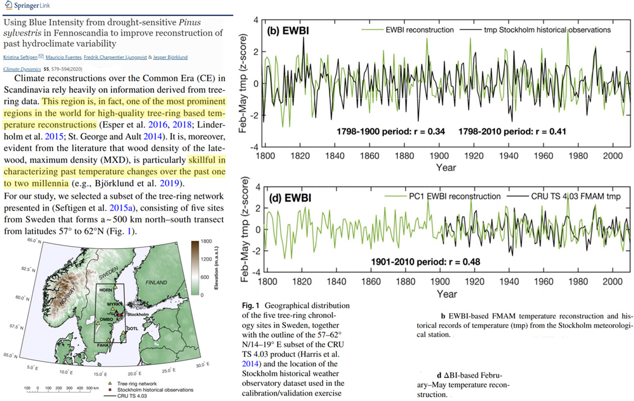
Seftigen et al., 2020 Sweden, no net warming 1800-2010
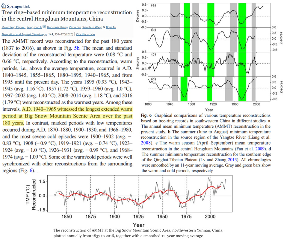
Keyimu et al., 2020 Hengduan Mtns, China longest extended warm period occurred in 1940-’65
A.D. 1940–1965 witnessed the longest extended warm period at Big Snow Mountain Scenic Area over the past 180 years
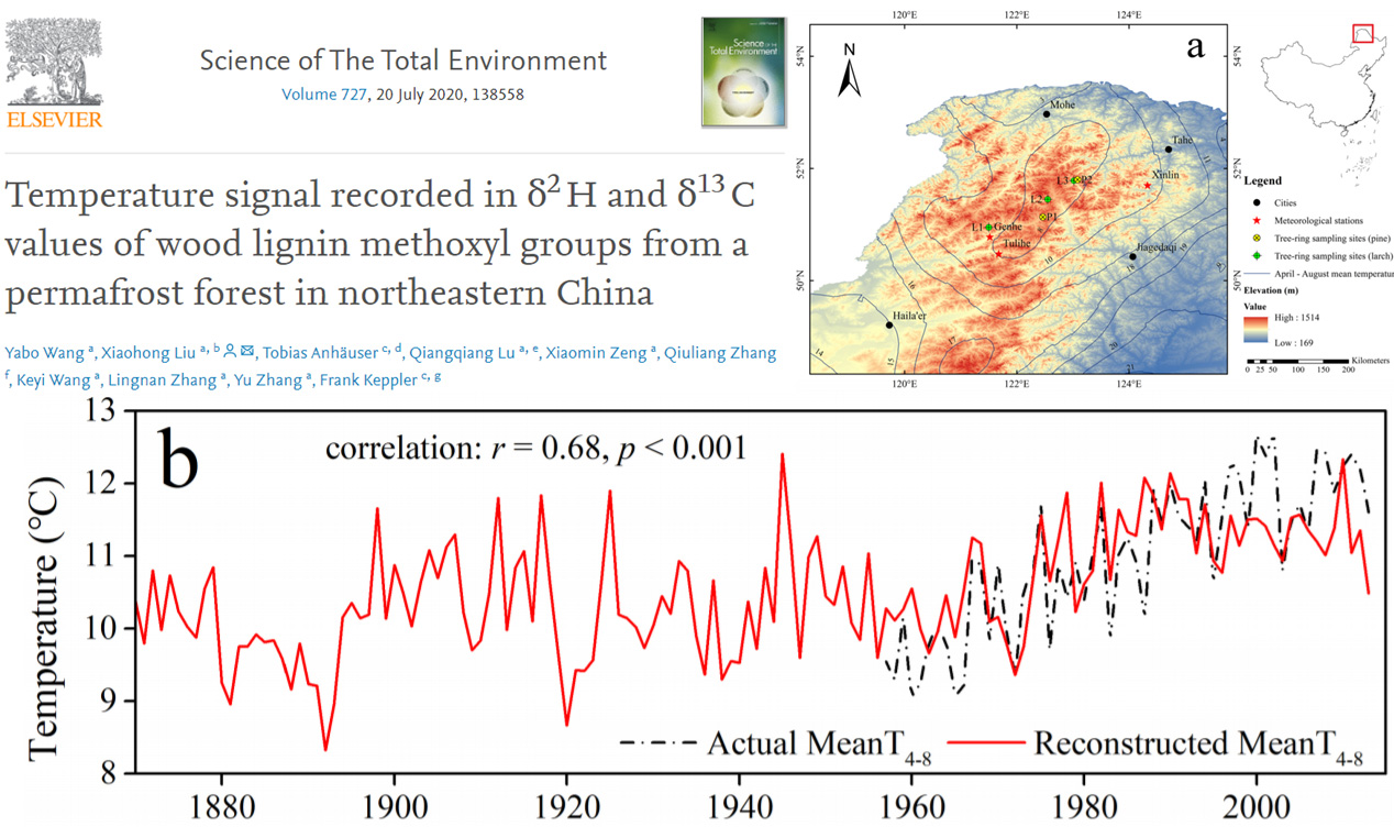
Wang et al., 2020 NE China cooling since the 1980s
From 1957 to 2013, the average temperature was −3.9°C (Figure 1c). The mean annual temperature increased by 0.9°C per decade from 1957 to 1990, but thereafter, it was stable (Figure 1c). The annual temperature variation (average monthly temperature) was extreme, ranging from −28.1°C in January to 17.3°C in July (Figure 1b).
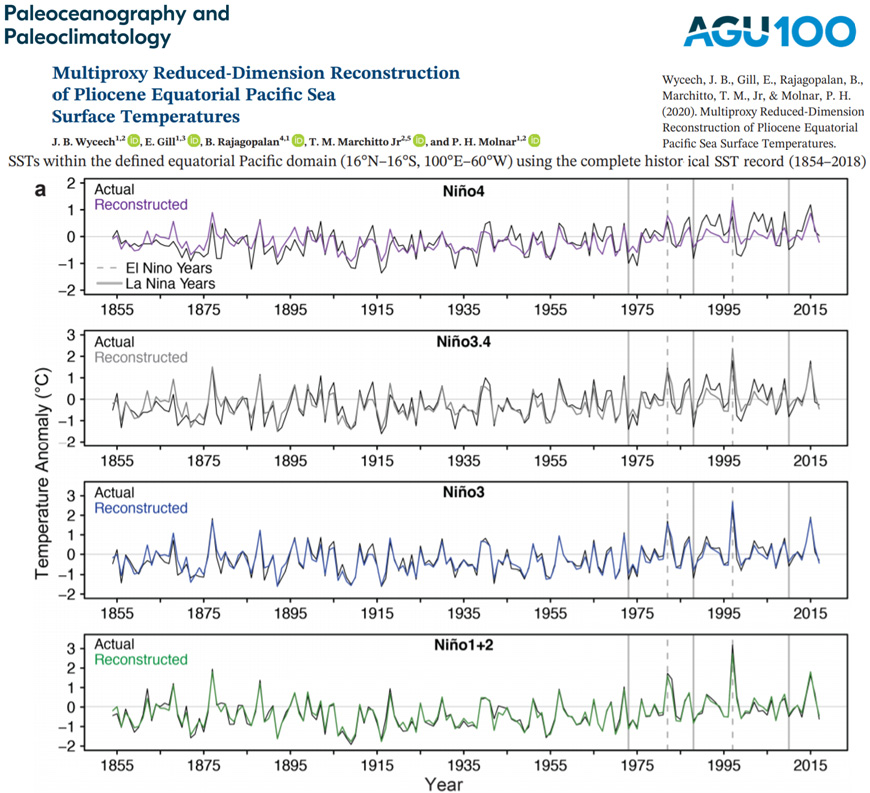
Wycech et al., 2020 Recent non-warming Eastern Equatorial Pacific SSTs
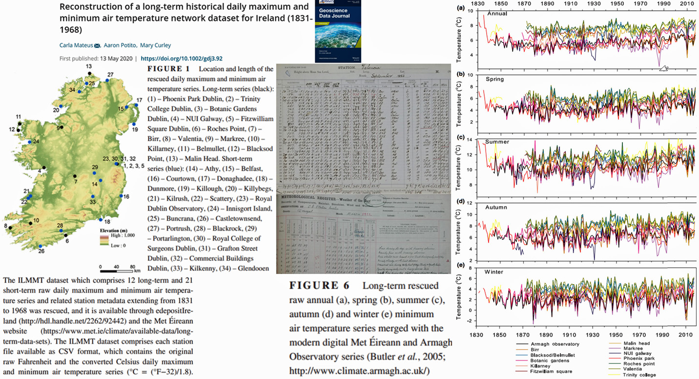
Mateus et al., 2020 Ireland, no apparent net warming since 1831
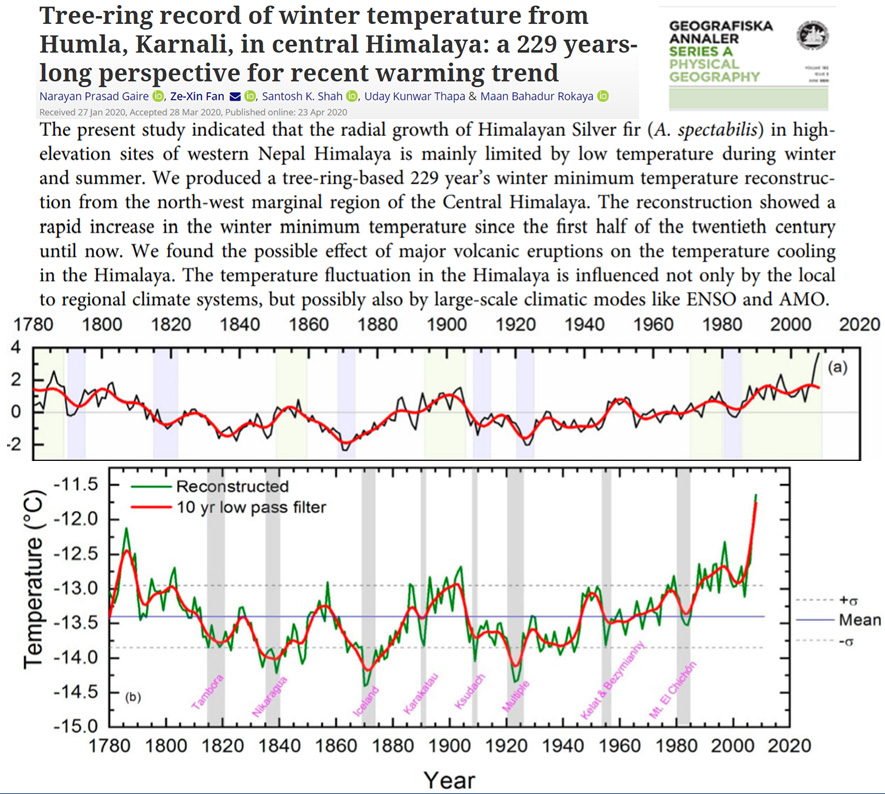
Gaire et al., 2020 Central Himalaya no net warming since 1780s
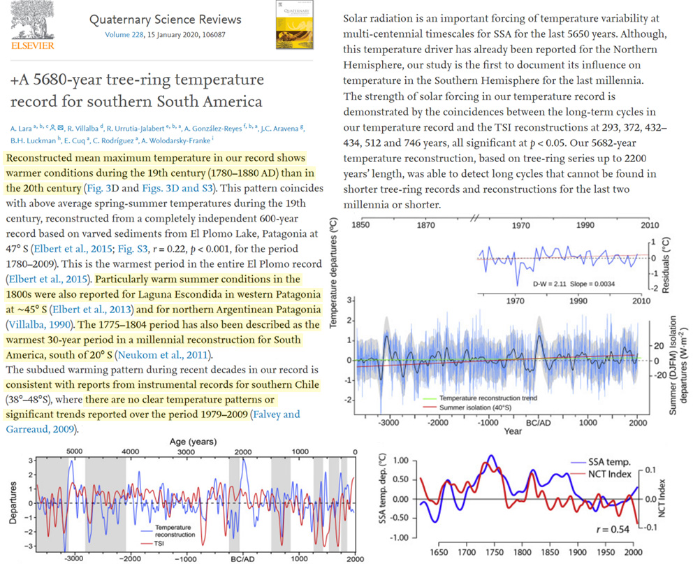
Lara et al., 2020 Southern South America warmer 1775-1884, no warming since 1979
The most outstanding features in the reconstruction presented here are two major warm periods between 3140–2800 BC and 70 BC – 150 AD (5159–4819 and 2089–1869 years ago, respectively, counted from 2019 to facilitate comparisons with glacier records based on 10Be dated moraines). During these warm periods, no glacier advances have been reported for Patagonia (Aniya, 2013; Kaplan et al., 2016; Strelin et al., 2014, Fig. 5A). … Reconstructed mean maximum temperature in our record shows warmer conditions during the 19th century (1780–1880 AD) than in the 20th century (Fig. 3D and Figs. 3D and S3). The 1775–1804 period has also been described as the warmest 30-year period in a millennial reconstruction for South America, south of 20° S (Neukom et al., 2011). … The subdued warming pattern during recent decades in our record is consistent with reports from instrumental records for southern Chile (38°–48°S), where there are no clear temperature patterns or significant trends reported over the period 1979–2009 (Falvey and Garreaud, 2009).
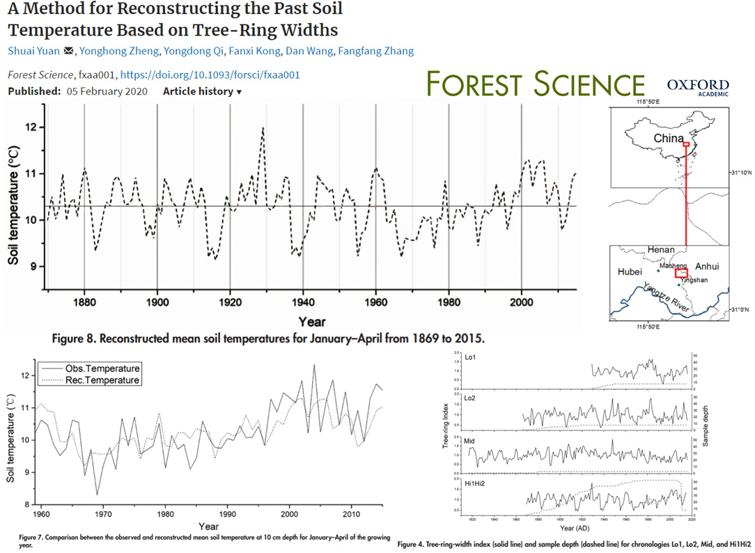
Yuan et al., 2020 SE China no warming since 1870
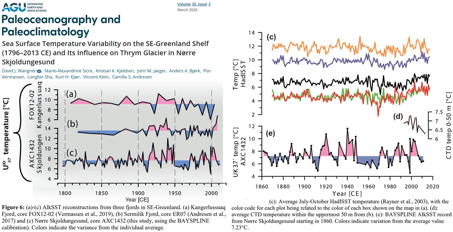
Wangner et al., 2020 SE Greenland warmer 1920s-1940s
The cold decades after 1950 coincide with the Great Salinity Anomaly in the late 60s to early 70s, caused by the long-term decrease of the North Atlantic Oscillation (NAO) index favoring the export of freshwater and ice through Fram Strait into the EGC (Dickson et al., 1996). Within two or three years, the associated salinity anomaly reached the Labrador Sea causing a reduction of the convection and subsequent weakening of the Atlantic Meridional Overturning Circulation (AMOC). This mechanism explains the low temperature on the SE-Greenland shelf and the positive AMV during this time period (Ionita et al., 2016, Figure 6d). … Displayed in the alkSST record from Skjoldungen as well as in the CTD measurements off Skjoldungen (Figure 5d) is a return to lower temperatures post 2006, pointing out the exceptional high temperatures around 2000. … Our study shows that even though the meltwater production may have been influenced by climate, the glacier margin position and iceberg calving remained relatively constant in the 20th century. This may be due to the setting of the glacier with a limited ice-ocean interface and a 90° inflow angle acting as a pinning point in its current position. Our study illustrates that ocean heat may have a limited effect on some marine glaciers.
Sun et al., 2020 NW China no warming since 1600s, cooling since 1950
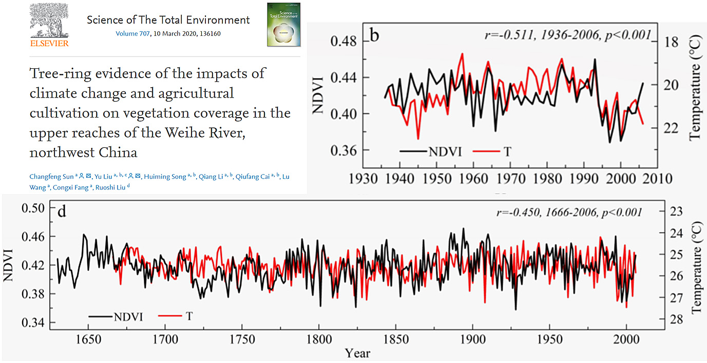
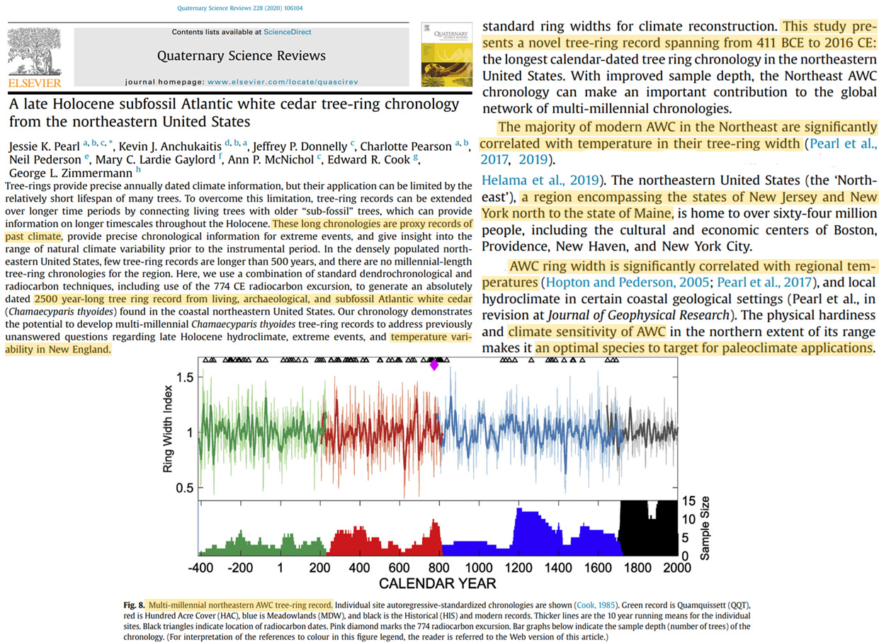
Pearl et al., 2020 NE USA no net warming from 411 BCE to 2016
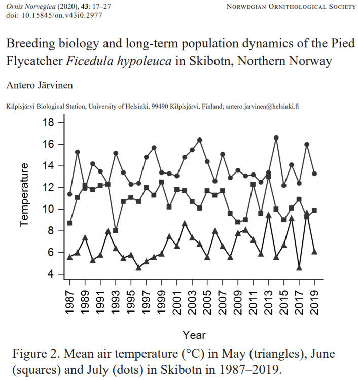
Järvinen, 2020 Recent non-warming, northern Norway
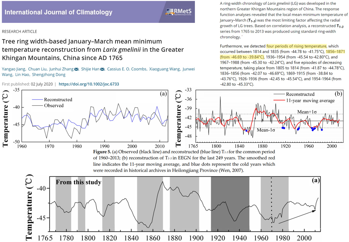
Jiang et al., 2020 Khingan Mountains (China) cooling since 1870s, 7°C warming 1856-’71
[W]e detected four periods of rising temperature, which occurred between 1814 and 1835 (from -44.78 to -41.75°C), 1856-1871 (from -46.69 to -39.84°C)
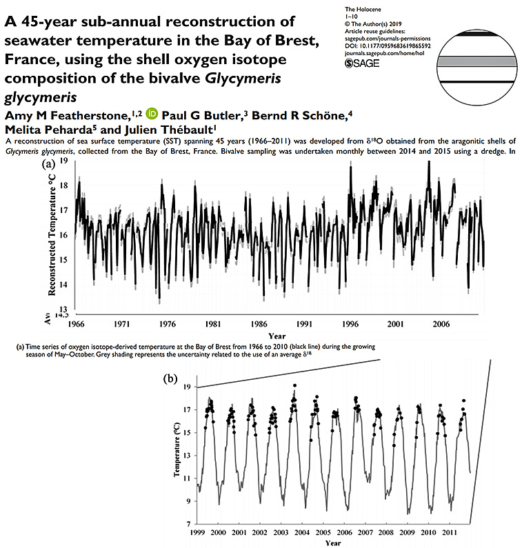
Featherstone et al., 2020 Recent non-warming, Bay of Brest, France
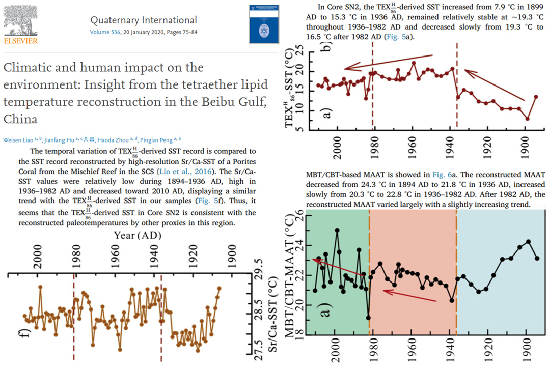
Liao et al., 2020 South China Sea recent (since 1940) non-warming/cooling
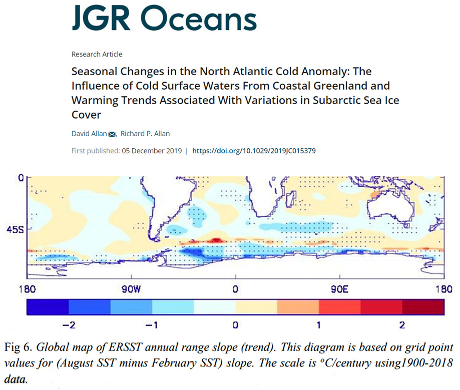
Allan and Allan, 2020 Southern Hemisphere: More cooling than warming from 1900-2018?
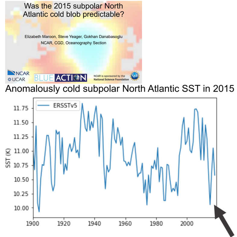
Although it is well-established that mean global SST has increased by about 1°C since 1900 (Huang et al 2017), a sector of the SPG centred near 50°N, 40°W has experienced a pronounced relative cooling approaching 1°C over the same period (Drijfhout et al 2012, Rahmstorf et al. 2015; Josey et al 2018; Caesar et al 2018 and Fig 2a). This almost unique region of long term surface cooling is sometimes referred to colloquially as the ‘cold blob’ (CB) (Rahmstorf et al 2015) when mapped as the regression of local SST changes relative to global mean values.
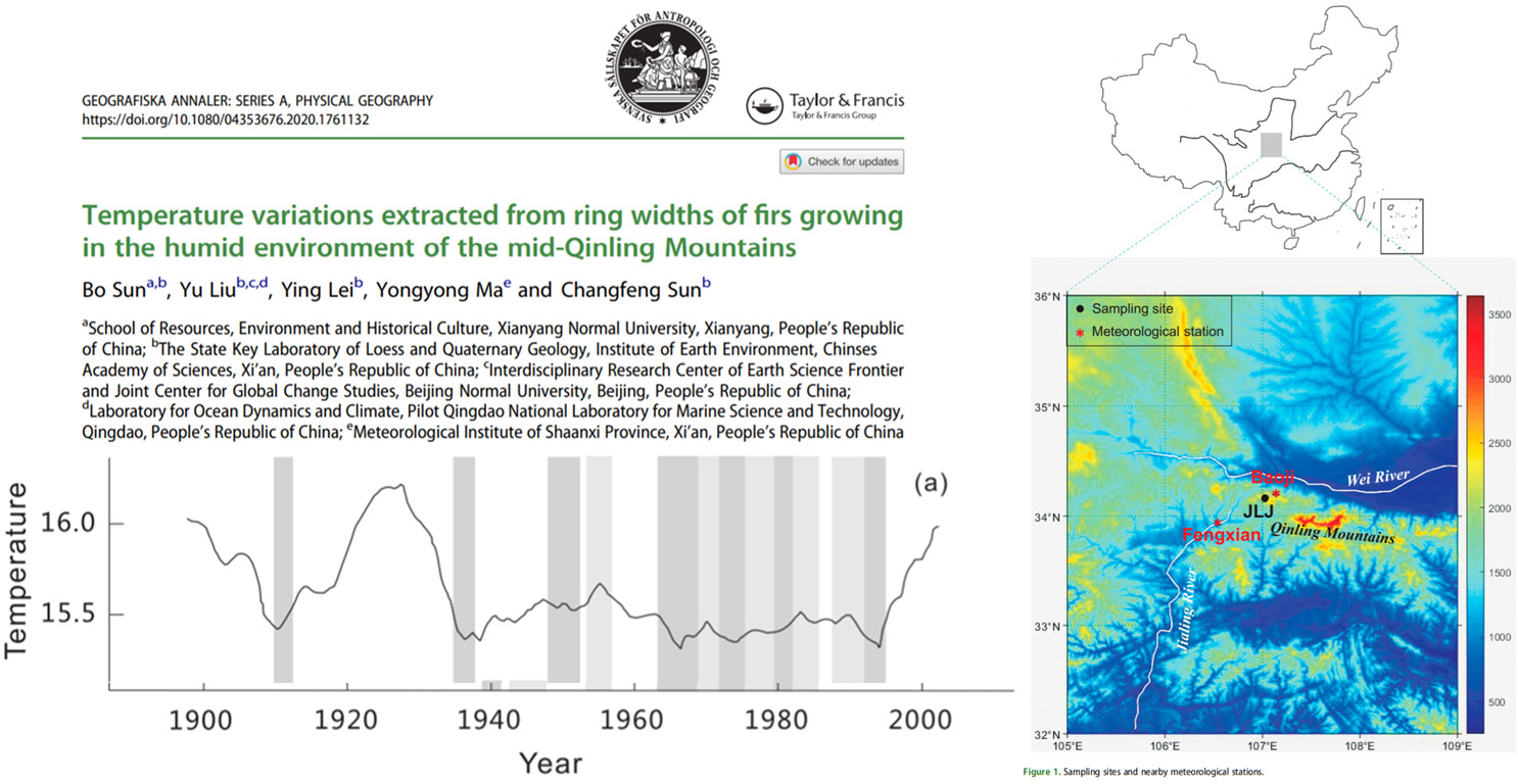
Sun et al., 2020 Central China (Qinling Mountains) warmer in the 1920s and 1930s
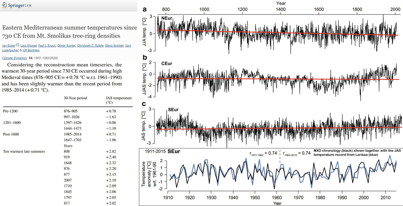
Esper et al., 2020 Warmest period in Europe “during high Medieval times” (876-905 CE)
Considering the reconstruction mean timeseries, the warmest 30-year period since 730 CE occurred during high Medieval times (876–905 CE=+0.78 °C w.r.t. 1961–1990) and has been slightly warmer than the recent period from 1985–2014 (+0.71 °C).
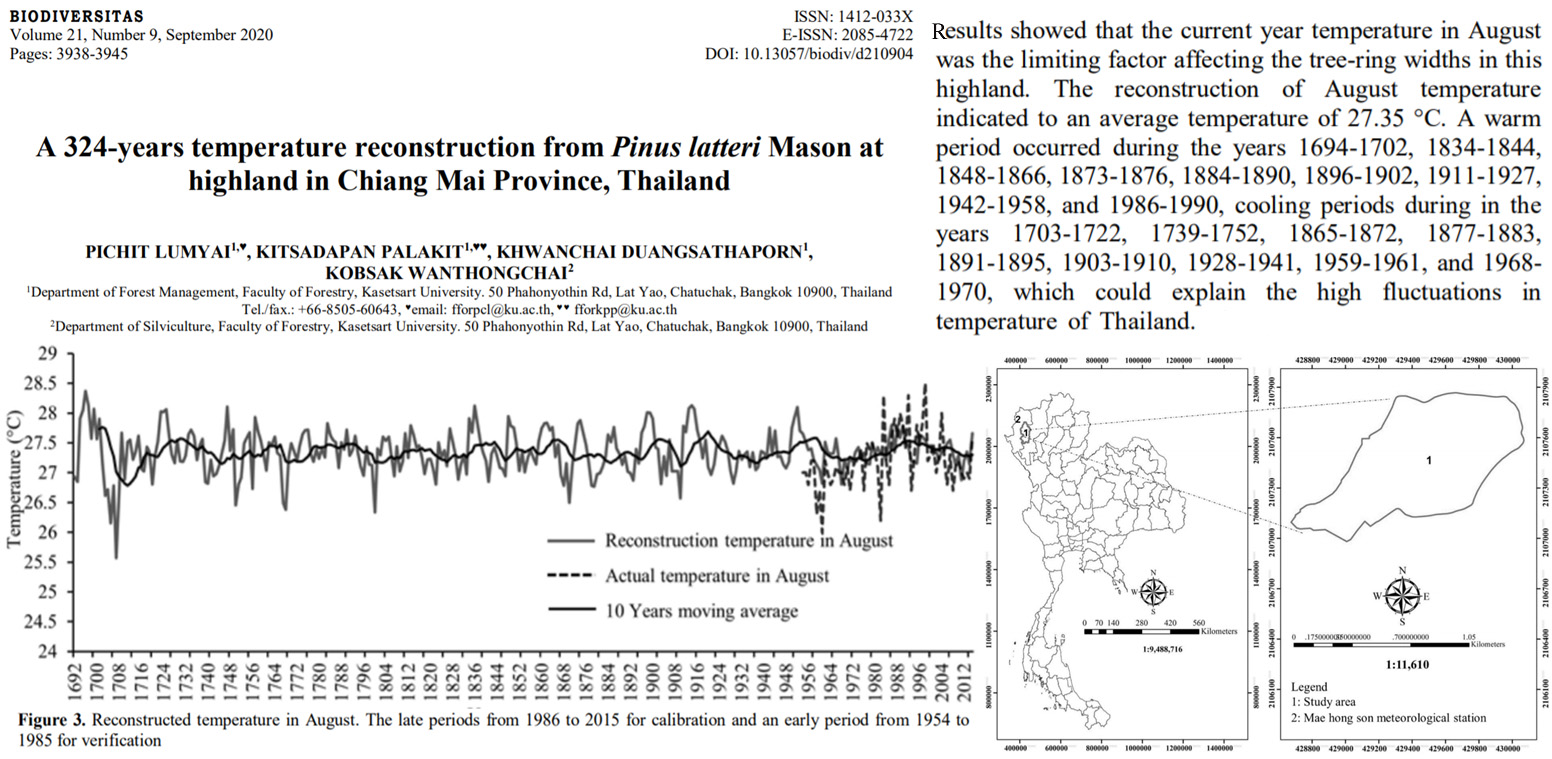
Lumyai et al., 2020 NW Thailand warmer in 1694-1702 than post-1990s
The results showed that the current year temperature in August was the limiting factor affecting the tree-ring widths in this highland. The reconstruction of August temperature indicated to an average temperature of 27.35°C. A warm period occurred during the years 1694-1702, 1834-1844, 1848-1866, 1873-1876, 1884-1890, 1896-1902, 1911-1927, 1942-1958, and 1986-1990.
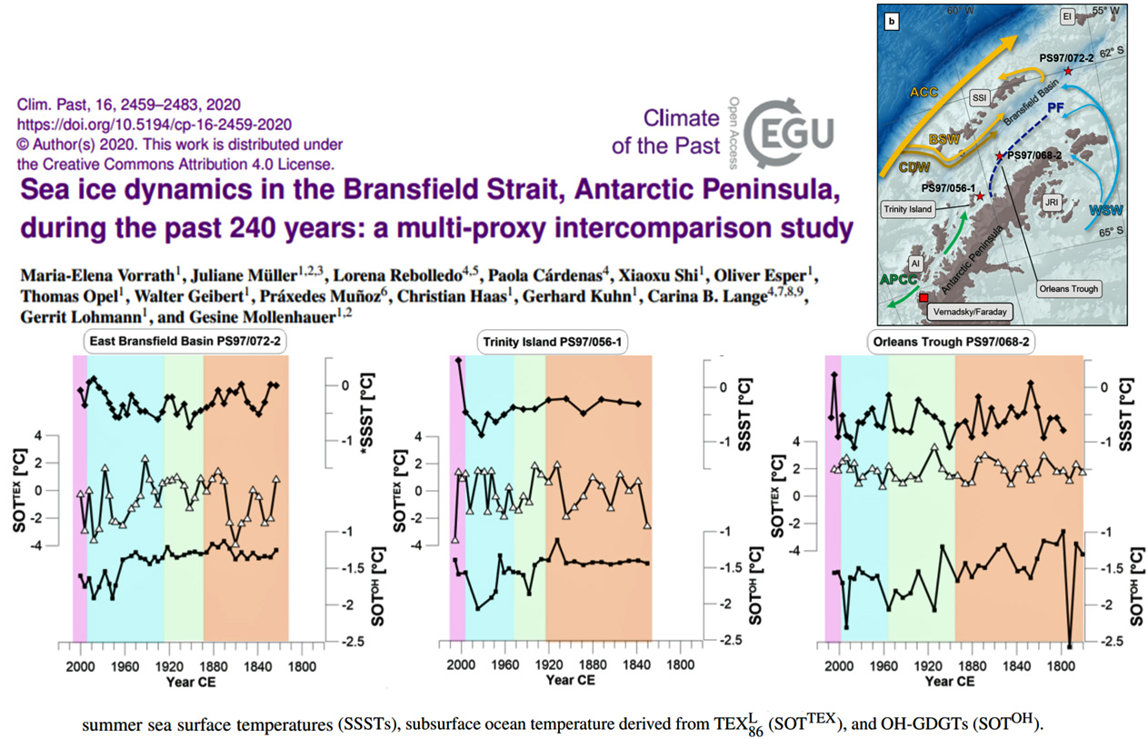
Vorrath et al., 2020 Antarctic Peninsula recent non-warming in 8 of 9 temp records
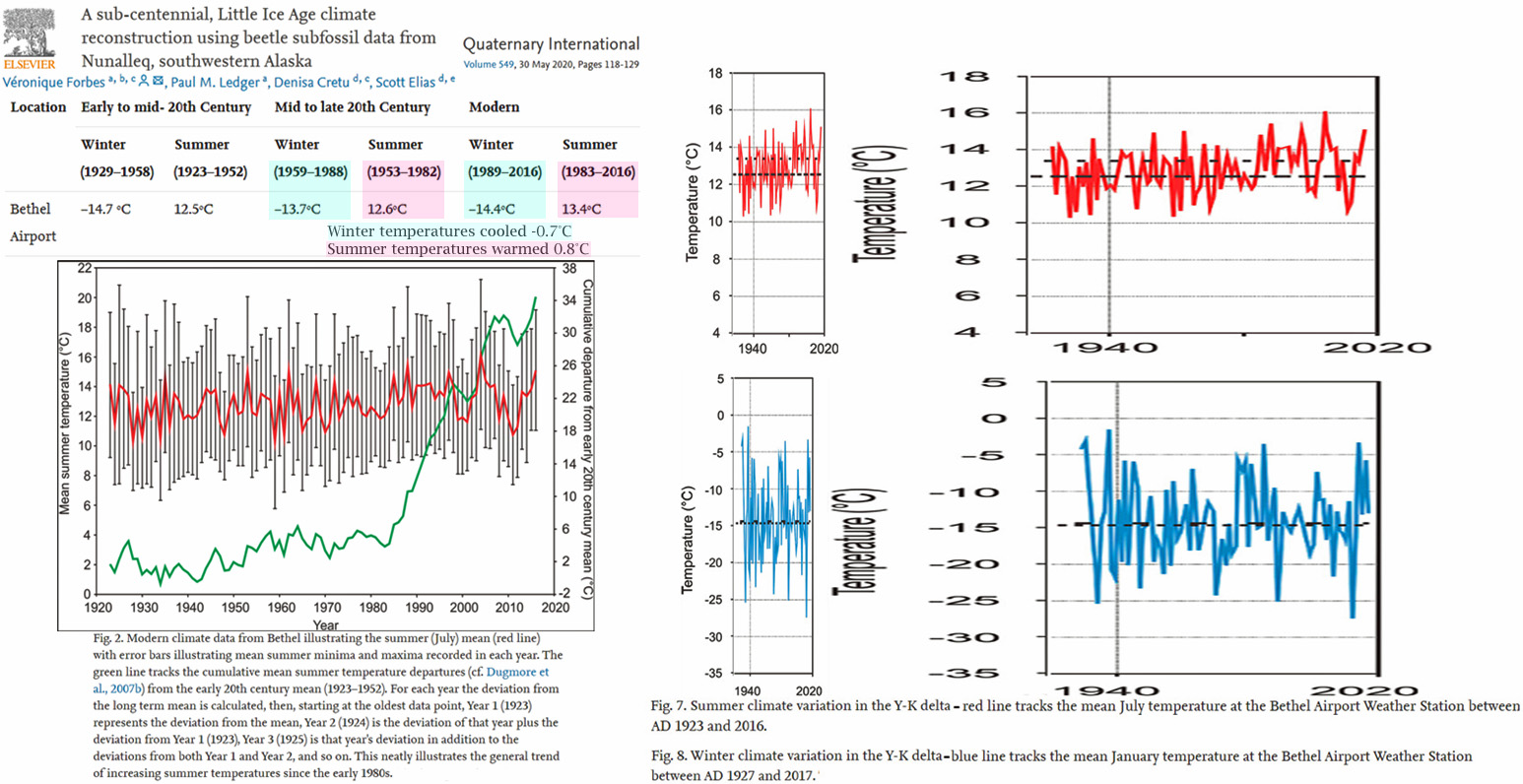
Forbes et al., 2020 SW Alaska winter temps cooled -0.7°C, summer temps warmed +0.8°C since 1950s
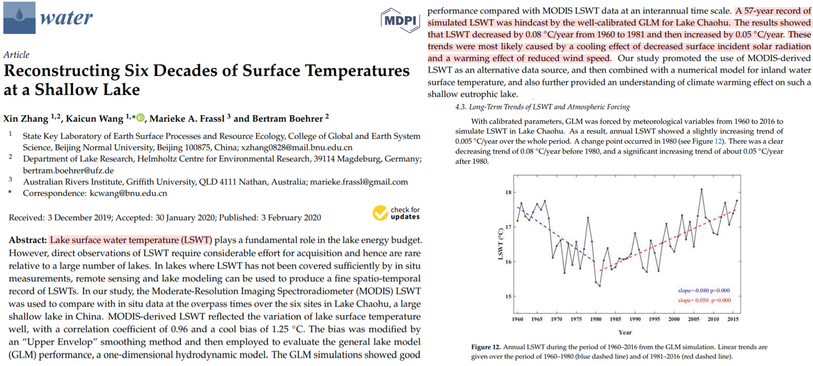
Zhang et al., 2020 China lake: -0.8°C per decade cooling 1960-1981 before +0.5°C/decade warming
The results showed that LSWT decreased by 0.08°C/year from 1960 to 1981 and then increased by 0.05°C/year. These trends were most likely caused by a cooling effect of decreased surface incident solar radiation and a warming effect of reduced wind speed.
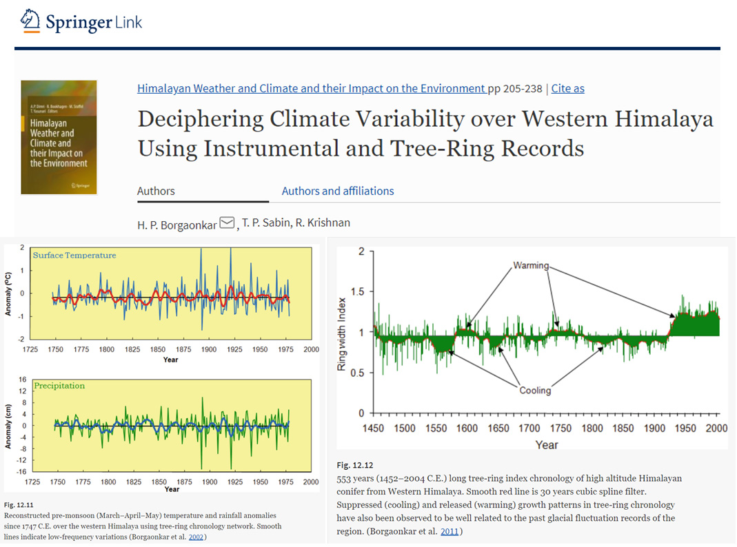
Borgaonkar et al., 2020 W. Himalaya no warming since ~1950s, “no…trend since past three centuries”
(Yadav et al. 2017) indicated increasing precipitation pattern and glacier expansion associated with cooling over northwest Himalaya. Similarly, reconstructed pre-monsoon (March–April–May) temperature and rainfall anomalies since 1747 C.E. over the western Himalaya using wide tree-ring chronology network did not show any increasing or decreasing trend since past three centuries (Fig. 12.11) (Borgaonkar et al. 2002).
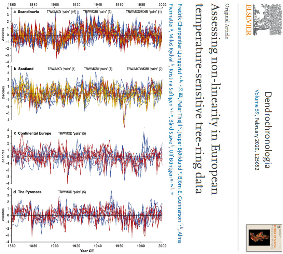
Ljungqvist et al., 2020 Scandinavia, Scotland, Europe, Pyrenees non-warming 1860-2000
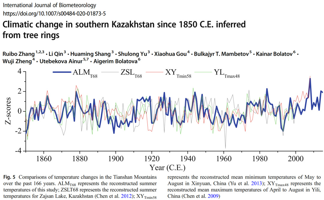
Zhang et al., 2020 Kazakhstan no net warming since 1850
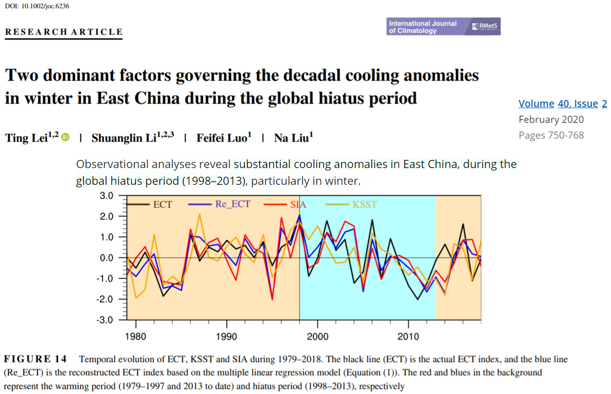
Lei et al., 2020 East China cooling during the global warming hiatus
Observational analyses reveal substantial cooling anomalies in East China, during the global hiatus period (1998–2013), particularly in winter.
Hua et al., 2020 Central China had two cold periods since 1853, including 1953-2000
With linear regression analysis, we reconstructed the March-April mean maximum temperature of Zhen’an over 165 years from 1853 to 2017. … [T]he reconstruction function and results were credible and reliable. Warm years occurred 25 times and cold years occurred 29 times in the reconstruction sequence. The warm years were more accompanied by flood events, while the cold years were accompanied by more drought events. Temperature fluctuated obviously in the reconstruction sequence, with two cold periods (1902-1917 and 1953-2000) and four warm periods (1868-1892, 1917-1937, 1941-1953 and 2001-2012).
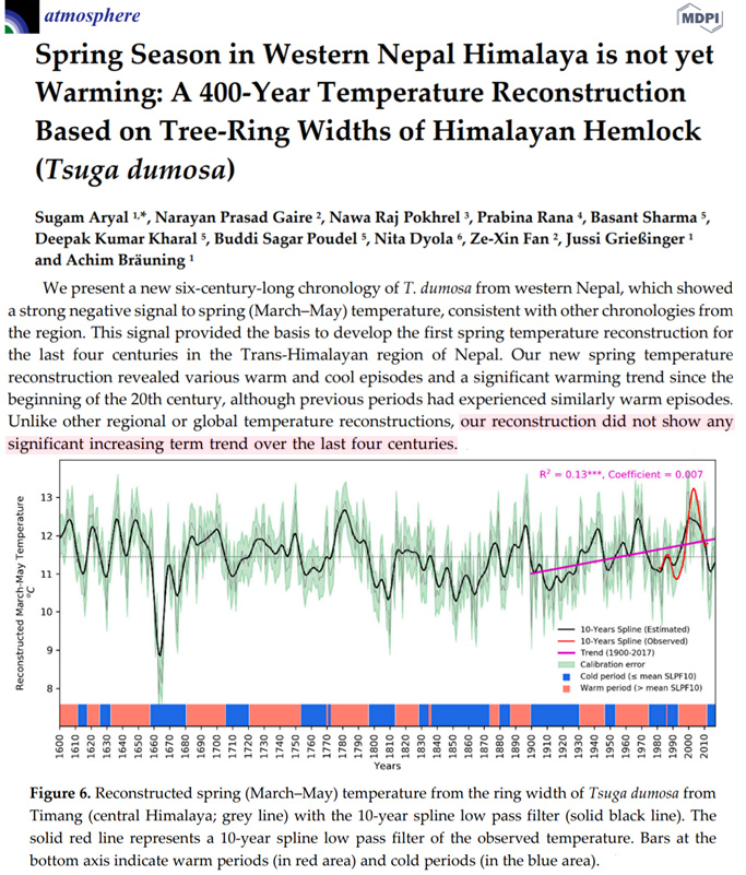
Aryal et al., 2020 Himalaya temps “did not show any significant increasing trend” in 400 yrs
Our new spring temperature reconstruction revealed various warm and cool episodes and a significant warming trend since the beginning of the 20th century, although previous periods had experienced similarly warm episodes. Unlike other regional or global temperature reconstructions, our reconstruction did not show any significant increasing term trend over the last four centuries. … The reconstructed spring temperature series contained periodicities that coincide with the periodicity of broader scale climate modes, such as AMO, NAO, and ENSO. This implies that the temperature in our study area is also regulated by broad‐scale atmospheric circulation patterns
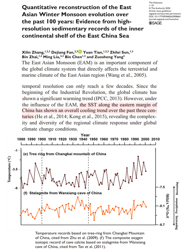
Zhang et al., 2020 East China Sea “an overall cooling trend over the past three centuries “
The East Asian Monsoon (EAM) is an important component of the global climate system that directly affects the terrestrial and marine climate of the East Asian region (Wang et al., 2005). … Since the beginning of the Industrial Revolution, the global climate has shown a significant warming trend (IPCC, 2013). However, under the influence of the EAM, the SST along the eastern margin of China has shown an overall cooling trend over the past three centuries (He et al., 2014; Kong et al., 2015), revealing the complexity and diversity of the regional climate response under global climate change conditions.
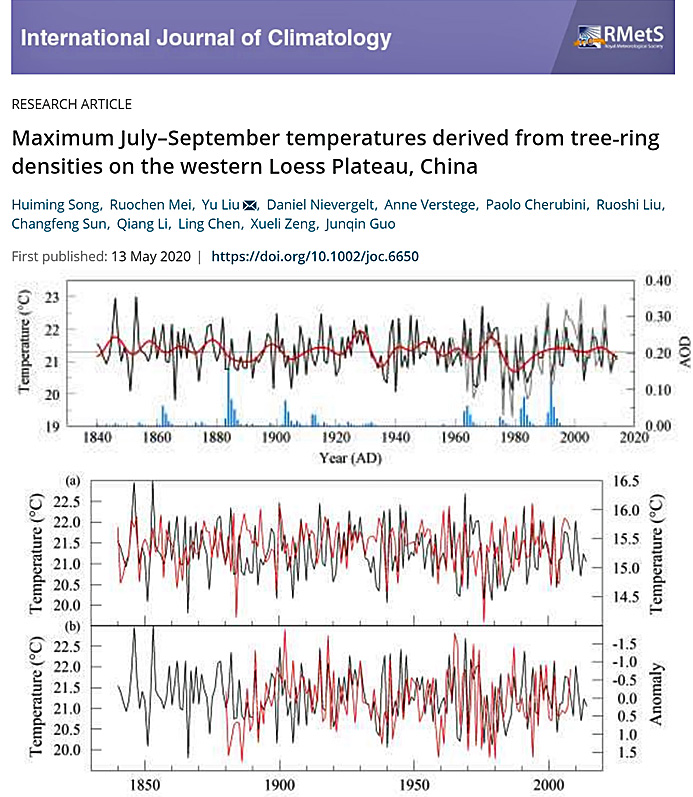
Song et al., 2020 Loess Plateau (China) cooling since 1840
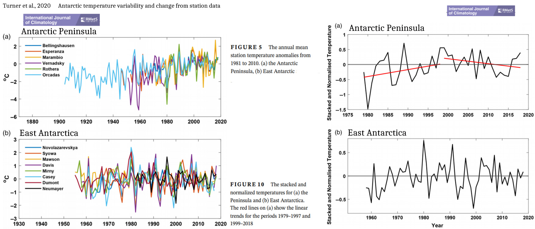
Turner et al., 2020 Antarctic Peninsula and East Antarctica recent cooling/non-warming
Haumann et al., 2020 Southern Ocean “unexpectedly” cooled -0.34°C from 1982-2011
Much of the Southern Ocean surface south of 55° S cooled and freshened between at least the early 1980s and the early 2010s [observation‐derived cooling of −0.34 ± 0.15 °C and freshening of −0.09 ± 0.01 PSU between 1982 and 2011]. Many processes have been proposed to explain the unexpected cooling, including increased winds or freshwater fluxes. However, these mechanisms so far failed to fully explain the surface trends and the concurrent subsurface warming (100 to 500 m). Here, we argue that these trends are predominantly caused by an increased wind‐driven northward sea‐ice transport, enhancing th extraction of freshwater near Antarctica and releasing it in the open ocean. … Antarctic sea‐ice changes thereby may have contributed to the slowdown of global surface warming over this period. Our conclusions are robust across all considered sensitivity cases, although the trend magnitude is sensitive to forcing uncertainties and the model’s mean state. It remains unclear whether these sea‐ice induced changes are associated with natural variability or reflect a response to anthropogenic forcing.
Johansson et al., 2020 West Greenland as warm in the 1930s as the 2000s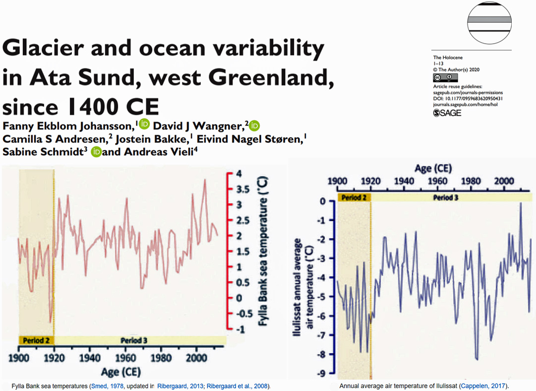
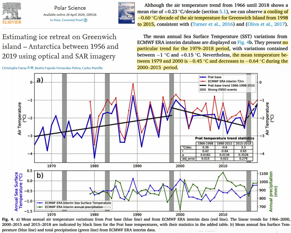
Fatras et al., 2020 Greenwich Island (Antarctica) cooling since 2000
The mean annual Sea Surface Temperature (SST) variations from ECMWF ERA interim database are displayed on Fig. 4b. They present no particular trend for the 1979–2018 period, with variations contained between -1°C and +0.15°C. Nevertheless, the mean temperature between 1979 and 2000 is -0.45°C and decreases to -0.64°C during the 2000–2015 period.
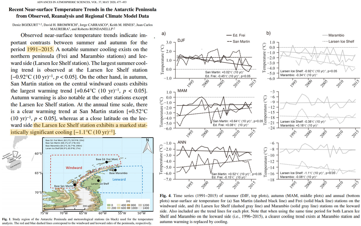
Bozkurt et al., 2020 Antarctic’s Larsen Ice Shelf cooling -1.1°C/decade since 1991
Observed near-surface temperature trends indicate important contrasts between summer and autumn for the period 1991−2015. A notable summer cooling exists on the northern peninsula (Frei and Marambio stations) and leeward side (Larsen Ice Shelf station). The largest summer cooling trend is observed at the Larsen Ice Shelf station [−0.92°C (10 yr)−1, p < 0.05]. On the other hand, in autumn, San Martin station on the central windward coasts exhibits the largest warming trend [+0.64°C (10 yr)−1 , p < 0.05]. Autumn warming is also notable at the other stations except the Larsen Ice Shelf station. At the annual time scale, there is a clear warming trend at San Martin station [+0.52°C (10 yr)−1 , p < 0.05], whereas at a close latitude on the leeward side the Larsen Ice Shelf station exhibits a marked statistically significant cooling [−1.1°C (10 yr)−1].
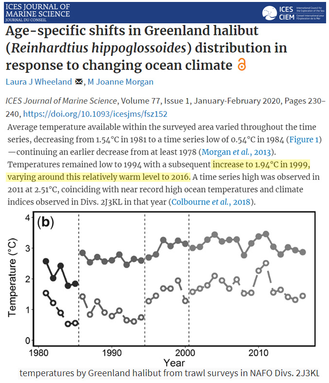
Wheeland and Morgan, 2020 Greenland no increasing temp trend 1999-2016
Huang et al., 2020 Some warming hiatuses (1989-2013) in China still ongoing
After five to 15 years of temperature increases (decreases) following the abrupt changes, warming (cooling) hiatuses occurred in some areas of China, with the hiatus years occurring between 1989 and 2013. These hiatuses mainly occurred in 1998 and 2007, and in terms of proximity, the stations without warming (cooling) hiatuses were concentrated south of 40° N. After nine to 17 years of warming (cooling) hiatuses, the hiatuses ended at some stations between 2013 and 2017, after which the temperatures again increased rapidly. The periods of warming (cooling) hiatuses were longer in northern China than in southern China. Currently, there are some stations where the hiatuses have not ended, suggesting that the hiatus period is apparently longer than 17 years. The years of abrupt change, no abrupt change, hiatus, no hiatus, end of hiatus, and no end of hiatus, as well as their variation trends before and after these years, have shown strong spatial variability.
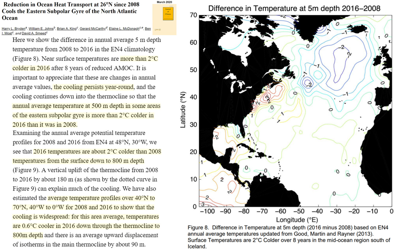
Bryden et al., 2020 North Atlantic cooled 2°C from 2008 to 2016
Here we show the difference in annual average 5 m depth temperature from 2008 to 2016 in the EN4 climatology (Figure 8). Near surface temperatures are more than 2°C colder in 2016 after 8 years of reduced AMOC. It is important to appreciate that these are changes in annual average values, the cooling persists year-round, and the cooling continues down into the thermocline so that the annual average temperature at 500 m depth in some areas of the eastern subpolar gyre is more than 2°C colder in 2016 than it was in 2008. … Examining the annual average potential temperature profiles for 2008 and 2016 from EN4 at 48°N, 30°W, we see that 2016 temperatures are about 2°C colder than 2008 temperatures from the surface down to 800 m depth (Figure 9). A vertical uplift of the thermocline from 2008 to 2016 by about 180 m (as shown by the dotted curve in Figure 9) can explain much of the cooling. We have also estimated the average temperature profiles over 40°N to 70°N, 40°W to 0°W for 2008 and 2016 to show that the cooling is widespread: for this area average, temperatures are 0.6°C cooler in 2016 down through the thermocline to 800m depth and there is an average upward displacement of isotherms in the main thermocline by about 90 m. (Figure 10). … There is a broad region of decreased net ocean heat loss extending southwest to northeast from the Bahamas toward Iceland with differences as large as 20 W m¯². Error maps for 5-year average NOC heat fluxes indicate uncertainties of order 5 W m¯² in this region well sampled by ships of opportunity (Berry and Kent, 2011, updated to 2015) so we consider these decreased ocean heat losses to be significant.
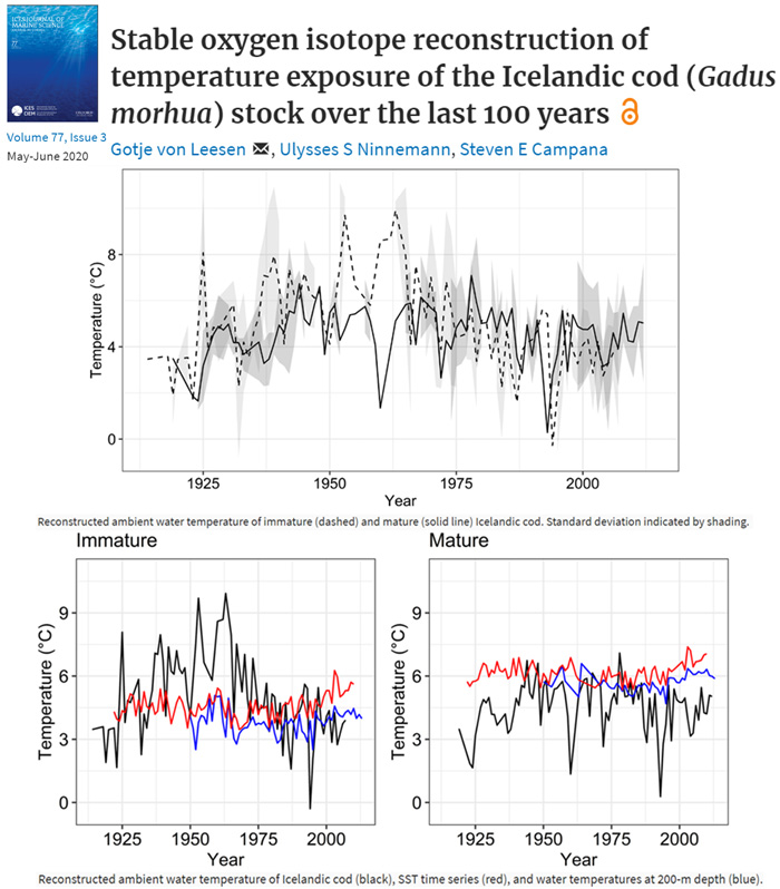
von Leesen et al., 2020 Iceland fishing waters cooling since the 1940s, 1950s
Cod were exposed to changing temperatures during the last 100 years … The overall trend over time was the same for both life stages, but immature cod were exposed to warmer temperatures than mature cod until 1980, when the ambient temperature of juveniles decreased. Since then, mature and immature cod have experienced similar water temperatures. The mean ambient temperature of all samples was 4.8°C: 4.9°C (−0.8 to 11.7°C) for juveniles and 4.6°C (−1.7 to 10.6°C) for adults.
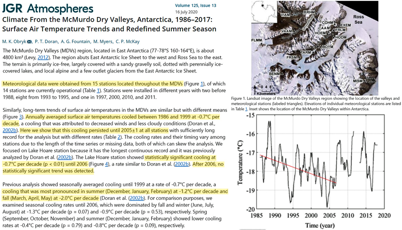
Obryk et al., 2020 East Antarctica cooling since 1986
The McMurdo Dry Valleys (MDVs) region, located in East Antarctica (77-78°S 160-164°E), is about 4800 km2 [Levy, 2012]. … Annually averaged surface air temperatures cooled between 1986 and 1999 at -0.7°C per decade, a cooling that was attributed to decreased winds and less cloudy conditions [Doran et al., 2002b]. Here we show that this cooling persisted until 2005±1 at all stations with sufficiently long record for the analysis but with different rates (Table 2). The cooling rates and their timing vary among stations due to the length of the time series or missing data, both of which can skew the analysis. We focused on Lake Hoare station because it has the longest continuous record and it was previously analyzed by Doran et al. [2002b]. The Lake Hoare station showed statistically significant cooling at -0.7°C per decade (p < 0.01) until 2006 (Figure 4), a rate similar to Doran et al. [2002b]. After 2006, no statistically significant trend was detected. … Previous analysis showed seasonally averaged cooling until 1999 at a rate of -0.7°C per decade, a cooling that was most pronounced in summer (December, January, February) at -1.2°C per decade and fall (March, April, May) at -2.0°C per decade [Doran et al., 2002b]. For comparison purposes, we examined seasonal cooling rates until 2006, which were dominated by fall and winter (June, July, August) at -1.3°C per decade (p = 0.07) and -0.9°C per decade (p = 0.53), respectively. Spring (September, October, November) and summer (December, January, February) showed lower cooling rates at -0.4°C per decade (p = 0.79) and -0.8°C per decade (p = 0.09), respectively.
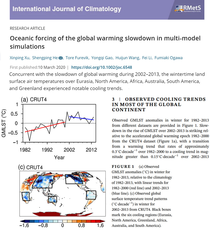
Xu et al., 2020 “Observed cooling trends in most of the global continent”
Concurrent with the slowdown of global warming during 2002–2013, the wintertime land surface air temperatures over Eurasia, North America, Africa, Australia, South America, and Greenland experienced notable cooling trends. … The slowdown concurs with a negative phase of the Pacific Decadal Oscillation (PDO), indicating that PDO plays an important role in modulating the global warming signal. Not all ensemble members capture the cooling trends over the continents, suggesting additional contribution from internal atmospheric variability.
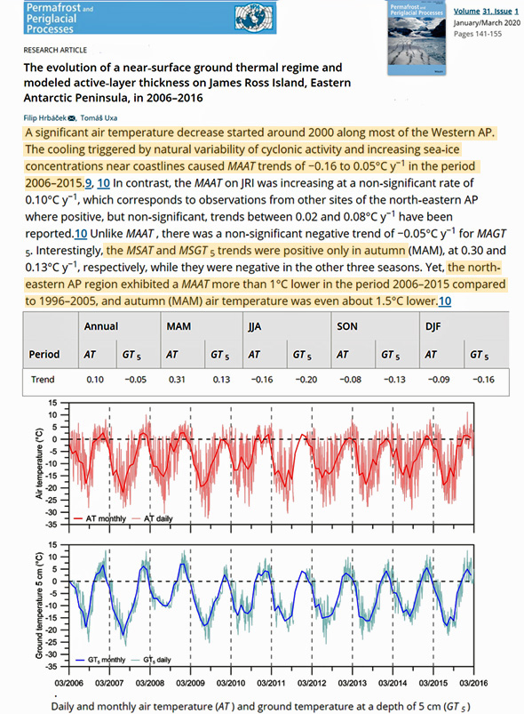
Hrbáček and Uxa, 2020 Eastern Antarctic Peninsula temps “1°C lower” in 2006-2015 vs. 1996-2005
A significant air temperature decrease started around 2000 along most of the Western AP. The cooling triggered by natural variability of cyclonic activity and increasing sea‐ice concentrations near coastlines caused MAAT trends of −0.16 to 0.05°C y−1 in the period 2006–2015. In contrast, the MAAT on JRI was increasing at a non‐significant rate of 0.10°C y−1, which corresponds to observations from other sites of the north‐eastern AP where positive, but non‐significant, trends between 0.02 and 0.08°C y−1 have been reported.10 Unlike MAAT , there was a non‐significant negative trend of −0.05°C y−1 for MAGT 5. Interestingly, the MSAT and MSGT 5 trends were positive only in autumn (MAM), at 0.30 and 0.13°C y−1, respectively, while they were negative in the other three seasons. Yet, the north‐eastern AP region exhibited a MAAT more than 1°C lower in the period 2006–2015 compared to 1996–2005, and autumn (MAM) air temperature was even about 1.5°C lower.
Maroon et al., 2020 Recent cooling subpolar North Atlantic – no net warming since 1900
Lack Of Anthropogenic/CO2 Signal In Sea Level Rise
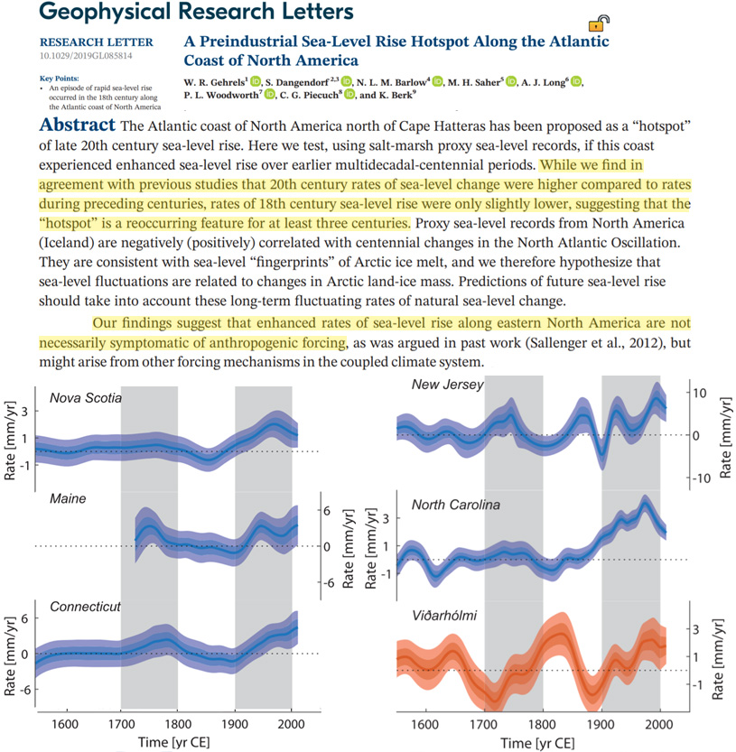
The Atlantic coast of North America north of Cape Hatteras has been proposed as a “hotspot”of late 20th century sea‐level rise. Here we test, using salt‐marsh proxy sea‐level records, if this coast experienced enhanced sea‐level rise over earlier multidecadal‐centennial periods. While we find in agreement with previous studies that 20th century rates of sea‐level change were higher compared to rates during preceding centuries, rates of 18th century sea‐level rise were only slightly lower, suggesting that the “hotspot” is a reoccurring feature for at least three centuries. Proxy sea‐level records from North America (Iceland) are negatively (positively) correlated with centennial changes in the North Atlantic Oscillation. They are consistent with sea‐level “fingerprints” of Arctic ice melt, and we therefore hypothesize that sea‐level fluctuations are related to changes in Arctic land‐ice mass. Predictions of future sea‐level rise should take into account these long‐term fluctuating rates of natural sea‐level change. … Our findings suggest that enhanced rates of sea‐level rise along eastern North America are not necessarily symptomatic of anthropogenic forcing, as was argued in past work (Sallenger et al., 2012), but might arise from other forcing mechanisms in the coupled climate system.
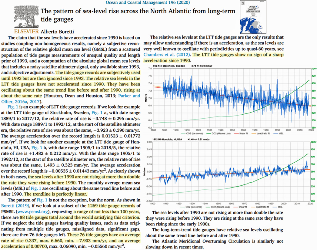
The claim that the sea levels have accelerated since 1990 is based on studies coupling non-homogeneous results, namely a subjective reconstruction of the relative global mean sea level (GMSL) from a scattered population of tide gauge measurements of unequal quality and length prior of 1993, and a computation of the absolute global mean sea levels that includes a noisy satellite altimeter signal, only available since 1993, and subjective adjustments. The tide gauge records are subjectively used until 1993 but are then ignored since 1993. The relative sea levels in the LTT tide gauges have not accelerated since 1990. They have been oscillating about the same trend line before and after 1990, rising at about the same rate (Houston, Dean and Houston, 2013; Parker and Ollier, 2016a, 2017).
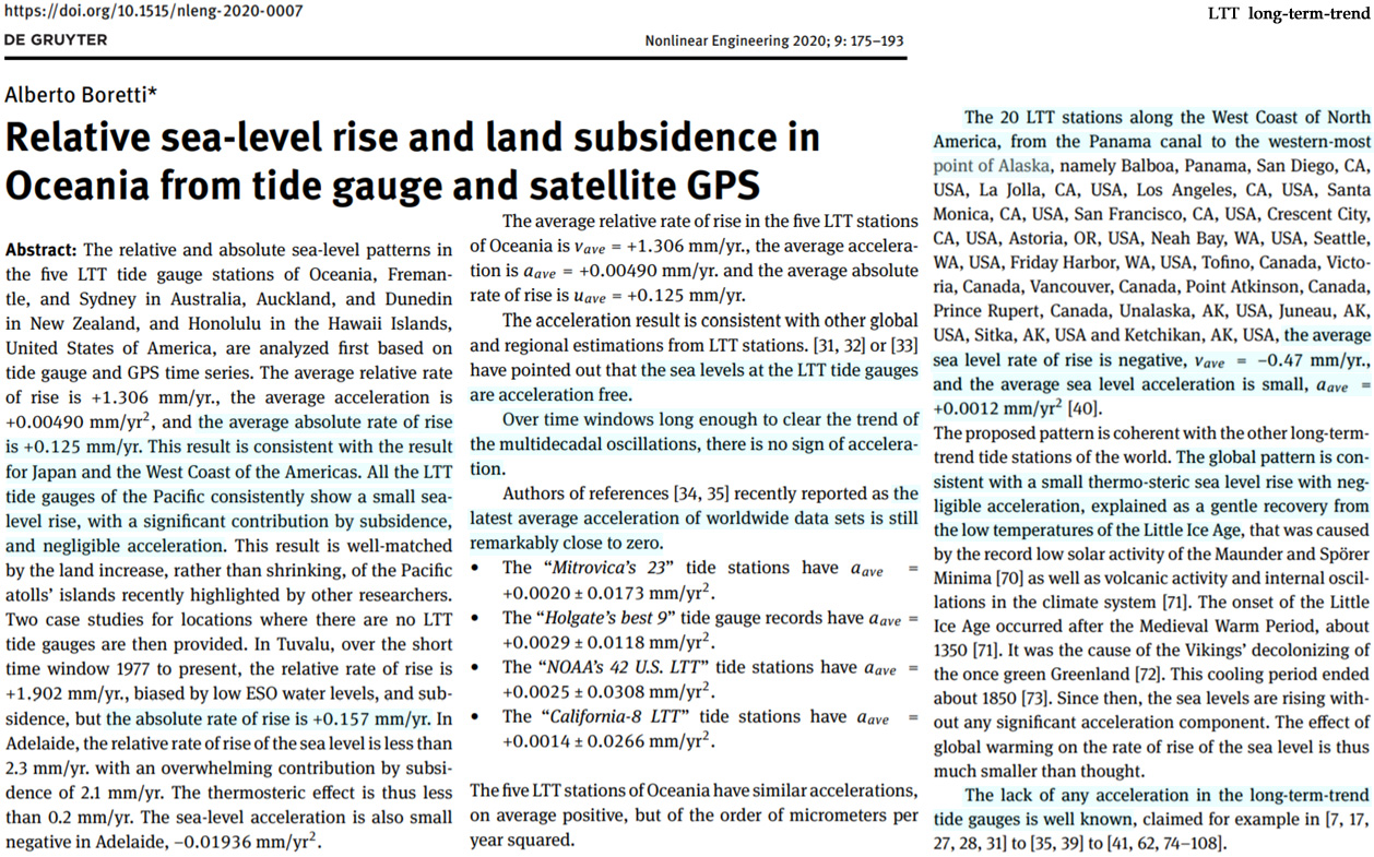
The relative and absolute sea-level patterns in the five LTT tide gauge stations of Oceania, Fremantle, and Sydney in Australia, Auckland, and Dunedin in New Zealand, and Honolulu in the Hawaii Islands, United States of America, are analyzed first based on tide gauge and GPS time series. The average relative rate of rise is +1.306 mm/yr., the average acceleration is +0.00490 mm/yr2, and the average absolute rate of rise is +0.125 mm/yr. This result is consistent with the result for Japan and the West Coast of the Americas. All the LTT tide gauges of the Pacific consistently show a small sea-level rise, with a significant contribution by subsidence, and negligible acceleration. This result is well-matched by the land increase, rather than shrinking, of the Pacific atolls’ islands recently highlighted by other researchers. Two case studies for locations where there are no LTT tide gauges are then provided. In Tuvalu, over the short time window 1977 to present, the relative rate of rise is +1.902 mm/yr., biased by low ESO water levels, and subsidence, but the absolute rate of rise is +0.157 mm/yr. In Adelaide, the relative rate of rise of the sea level is less than 2.3 mm/yr. with an overwhelming contribution by subsidence of 2.1 mm/yr. The thermosteric effect is thus less than 0.2 mm/yr. The sea-level acceleration is also small negative in Adelaide, −0.01936 mm/yr2.
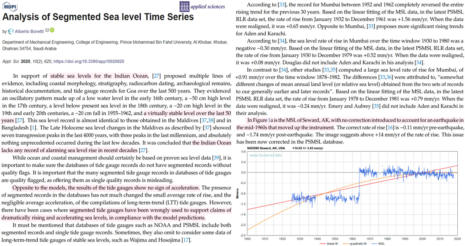
The Late Holocene sea level changes in the Maldives as described by [37] showed seven transgression peaks in the last 4000 years, with three peaks in the last millennium, and absolutely nothing unprecedented occurred during the last few decades. It was concluded that the Indian Ocean lacks any record of alarming sea level rise in recent decades [27]. … Opposite to the models, the results of the tide gauges show no sign of acceleration. The presence of segmented records in the databases has not much changed the small average rate of rise, and the negligible average acceleration, of the compilations of long-term-trend (LTT) tide gauges. However, there have been cases where segmented tide gauges have been wrongly used to support claims of dramatically rising and accelerating sea levels, in compliance with the model predictions.
Increased flooding due to sea level rise (SLR) is expected to render reef islands, defined as sandy or gravel islands on top of coral reef platforms, uninhabitable within decades. Such projections generally assume that reef islands are geologically inert landforms unable to adjust morphologically. We present numerical modeling results that show reef islands composed of gravel material are morphodynamically resilient landforms that evolve under SLR by accreting to maintain positive freeboard while retreating lagoonward. Such island adjustment is driven by wave overtopping processes transferring sediment from the beachface to the island surface. Our results indicate that such natural adaptation of reef islands may provide an alternative future trajectory that can potentially support near-term habitability on some islands, albeit with additional management challenges.
[O]ver the past three to five decades, only 11.4 % of the 709 documented Indo-Pacific islands decreased in size, whereas 15.5 % increased and 73.1 % remained stable in area (Duvat, 2019). … These studies investigating short-term island changes thus emphasized two key points: first, the high variability of island behavior (erosion, stability, accretion) depending on the local context; and second, the prominent contribution of natural drivers to observed changes. … These studies investigating short-term island changes thus emphasized two key points: first, the high variability of island behavior (erosion, stability, accretion) depending on the local context; and second, the prominent contribution of natural drivers to observed changes. … Over the past decade, 59.1 % of islands (110 islands, including 62 inhabited and 48 resort islands) increased in size, whereas 38.2 % (71 islands, including 42 inhabited and 29 resort islands) were stable and only 2.7 % (5 resort islands) decreased in size.
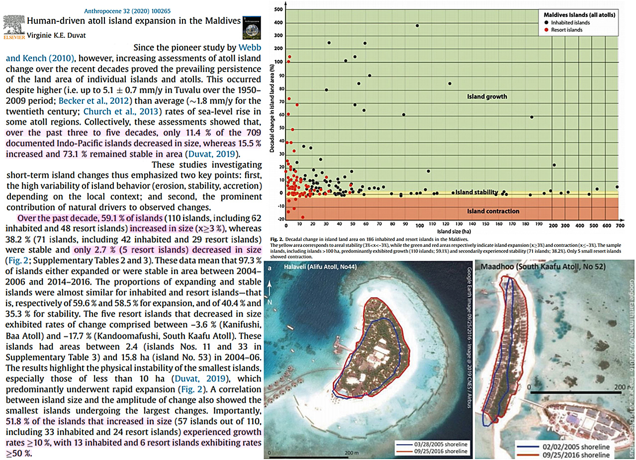
Microatoll growth is constrained by low water levels and, consequently, they are robust recorders of past sea level. U–Th dating of the Maldivian corals identified lowstands at AD 234–605 and AD 1481–1807 when sea level fell to maximum depths of −0.88 m and −0.89 m respectively. These lowstands are synchronous with reductions in radiative forcing and sea surface temperature associated with the Late Antiquity Little Ice Age and the Little Ice Age. Our results provide high-fidelity observations of lower sea levels during these cool periods and show rates of change of up to 4.24 mm yr−1. Our data also confirm the acceleration of relative sea-level rise over the past two centuries and suggest that the current magnitude and rate of sea-level rise is not unprecedented.
The average SLR,rel at the long term trend world tide gauges is similarly less than SLR,rel = 0.5 mm yr−1 (Parker & Ollier, 2016, 2017). The average acceleration is a few μm·yr−2 (Parker & Ollier, 2016, 2017). The lack of any acceleration in the tide gauges’ signals is well-known in the literature, (Boretti, 2012; Douglas, 1992; Douglas and Peltier, 2002; De Lange and Carter, 2014; Fasullo et al., 2016; Houston and Dean, 2011; Mörner, 2004, 2013; Parker & Ollier, 2016, 2017; Idso et al., 2014).Other indicators, such as the increasing, rather than shrinking, areas of the emerged atoll islands in the Pacific or the Indian ocean (Duvat, 2019; Aslam and Kench, 2017; Kench et al., 2015; Webb and Kench, 2010) support this stable sea level pattern indicated by the long term trend tide gauge records.
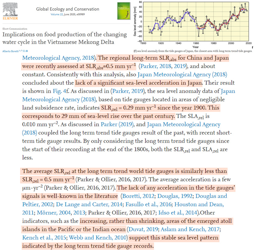
The 25-year record of satellite-altimeter measured sea-level has led to improvements in the understanding of sea-level change on both regional and global scales. However, the extent to which the pattern of regional sea-level rise measured by altimeters is representative of the forced sea-level response remains an open question. Internal variability both contributes to regional sea-level changes on short timescales and masks the pattern of forced trend and acceleration associated with anthropogenic global warming. … While the dominant features in the acceleration pattern can be attributed to internal variability, there is an indication that the forced acceleration pattern may emerge as the record continues to lengthen. … Studies in recent years have convincingly shown that the altimeter-measured trends are heavily influenced by internal variability [e.g. Hamlington et al., 2014; Han et al., 2017; Bromirski et al., 2011; Hamlington et al., 2016]. … Here, we demonstrate that with the current length of the altimeter record, and accounting for and removing internal variability, the spatial variability of accelerations is, at least, reduced. Consistent with other studies, however, most locations do not display a significant acceleration, and many locations that do are likely still influenced by unaccounted for internal variability. … Although areas of moderate acceleration and deceleration are still present in Fig. 3d, most of the strong signals in Fig. 3b are dampened. There are two implications of this dampening: 1) for most locations across the globe, a significant acceleration or deceleration still has not emerged, despite removing some amount of internal variability; and 2) many of the large amplitude signals have been removed, narrowing the range of accelerations that could be associated with a forced response.
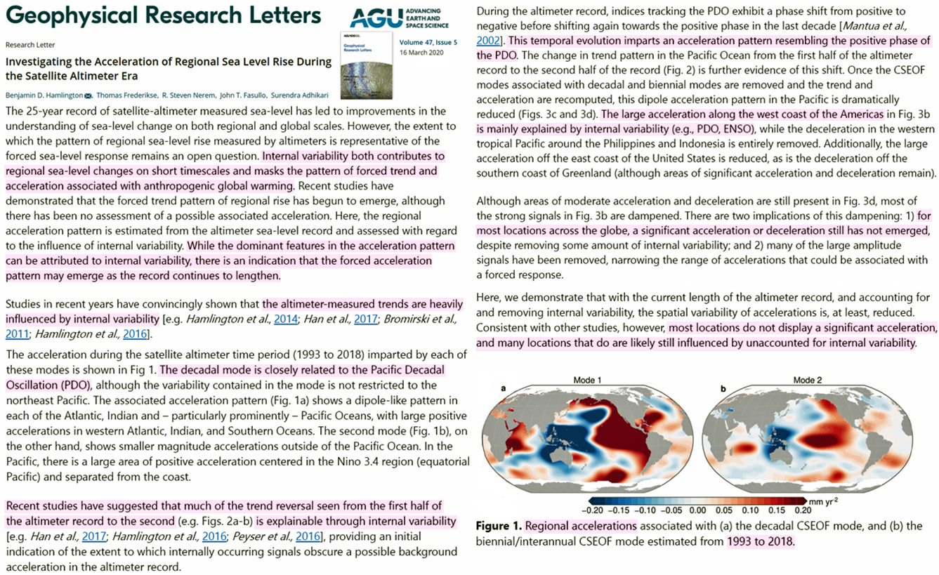
NY City relative sea-level rate of rise is -2.851 to -4.076 mm/yr. NY City GNSS subsidence is -2.151 to -3.076 mm/yr. NY City absolute sea level rate of rise is 0.7 to 1.0 mm/yr. NY City relative sea-level acceleration is about +0.008 mm/yr² … Although the climate models predict that rising CO2 levels should cause an accelerated sea-level rise, the sea level measurements show that, thus far, there has been no detectable acceleration in the rate of sea-level rise.
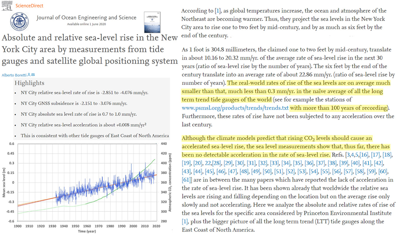
Over the past 30 years, despite sea-level rise, deltas globally have experienced a net land gain of 54 ± 12 square kilometres per year (2 standard deviations), with the largest 1 per cent of deltas being responsible for 30 per cent of all net land area gains. Humans are a considerable driver of these net land gains—25 per cent of delta growth can be attributed to deforestation-induced increases in fuvial sediment supply.
Ice-mass loss—predominantly from glaciers—has caused twice as much sea-level rise since 1900 as has thermal expansion. Mass loss from glaciers and the Greenland Ice Sheet explains the high rates of global sea-level rise during the 1940s … Our GMSL estimate (Fig. 1a) shows a trend of 1.56 ± 0.33 mm yr−1 (90% confidence interval) over 1900–2018. It is also characterized by substantial multidecadal variability, with higher rates of sea-level rise during the 1940s and since the 1990s, and lower rates around 1920 and 1970. … Thermosteric and barystatic sea-level changes show similar multidecadal variability patterns to the GMSL changes, although the amplitude of barystatic variability is larger than that of thermosteric variability, and barystatic variability is the main cause of multidecadal GMSL variability.
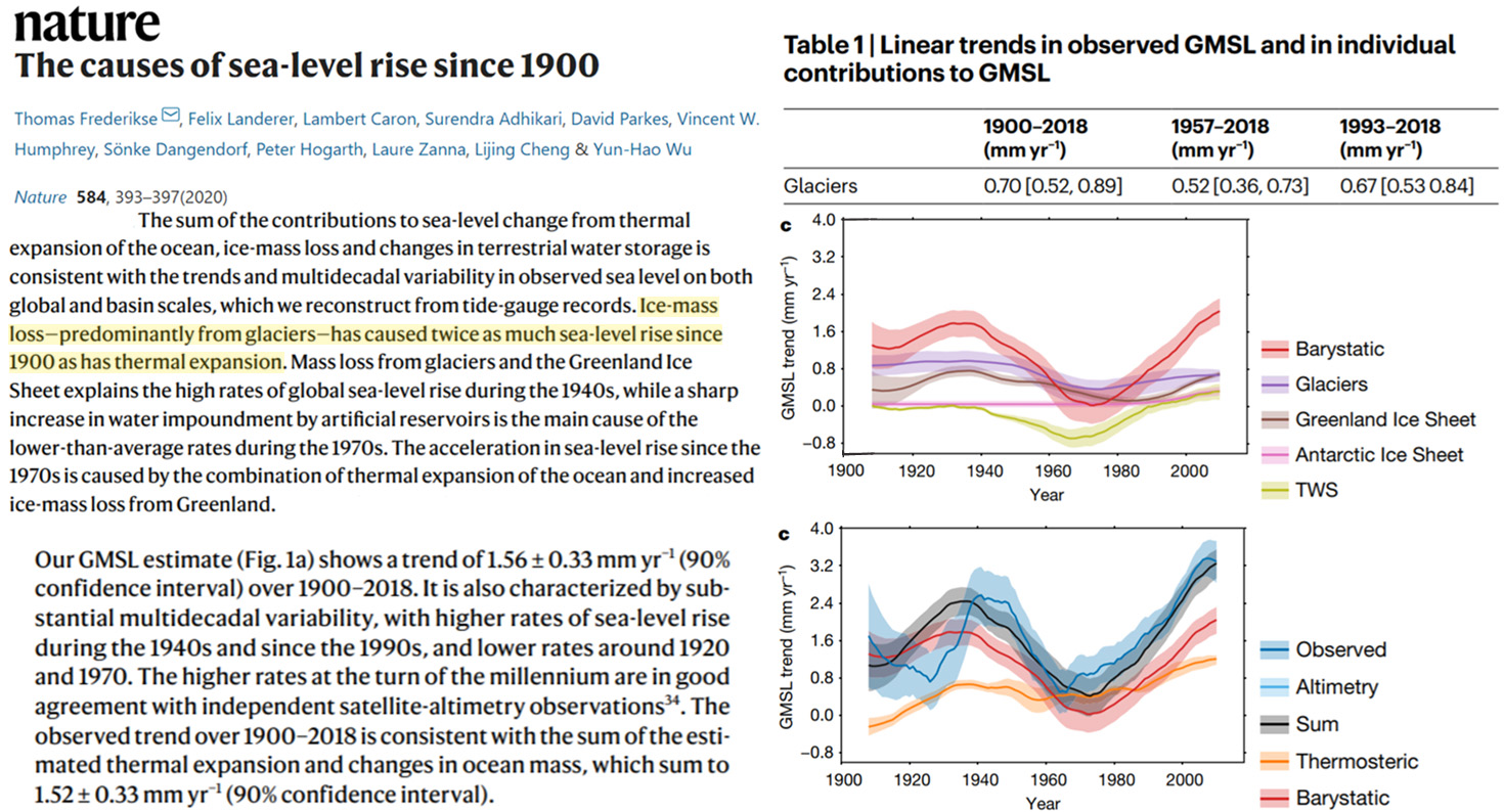
Sea Levels Meters Higher When CO2 <280 ppm
Leonard et al., 2020 Great Barrier Reef, +0.7 to 1 m higher than present
“[L]ate-Holocene relative sea level highstand of ~1 m at ~2000 yr. BP … “Relative sea level was also 0.7 m-1.0 m higher than present between 6200 and 5500 yr. BP“
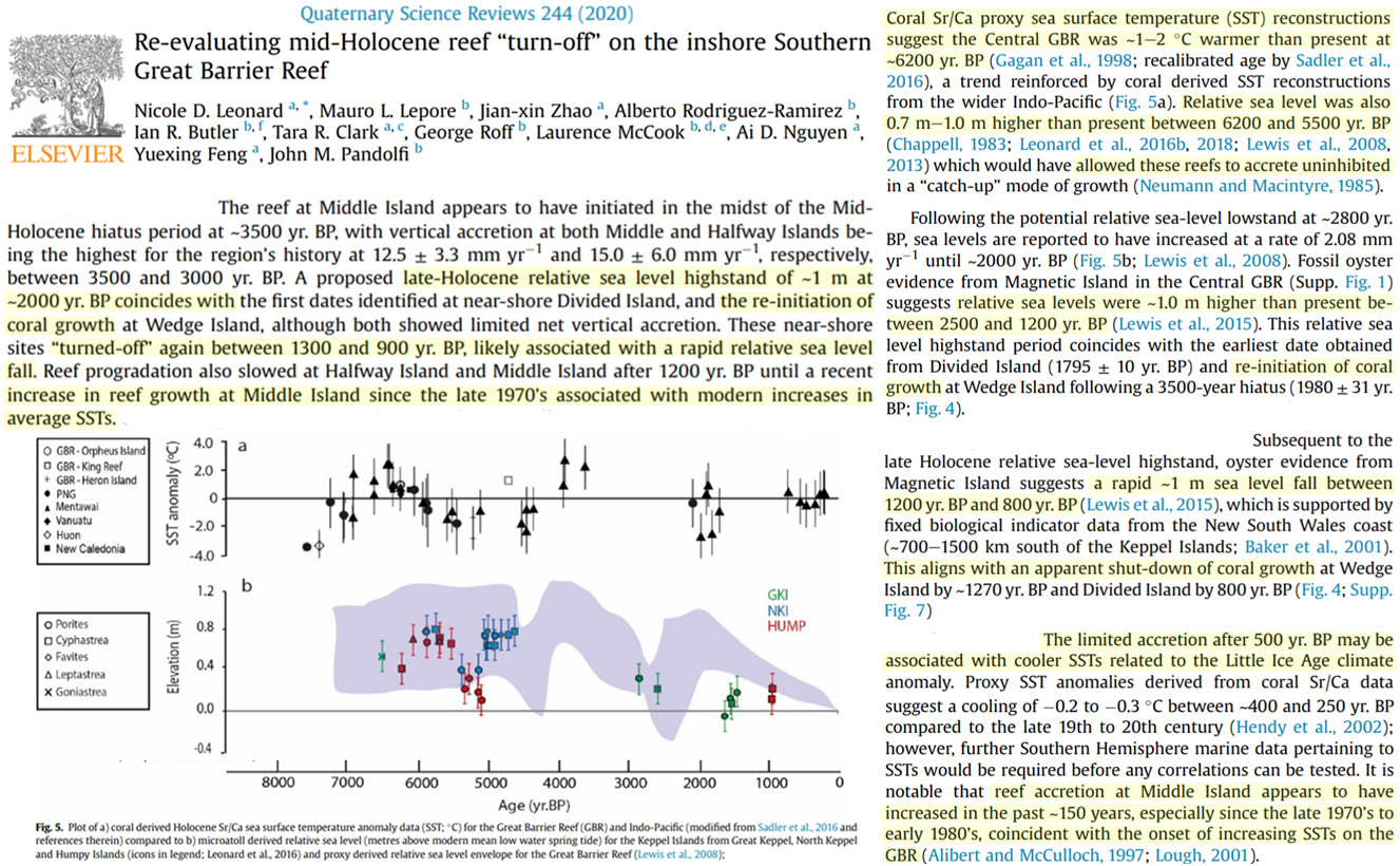
Kench et al., 2020 Maldives, +0.5 m higher than present
“Evident is the temporal disjuncture between the age and depth of dated corals, and island sediments, that provide insights into the staged development of Vaadhoo. In particular, island ages cluster in a 1000 year period (~2500–1500 yrs) synchronous with a marked transition in sea level from the mid-Holocene highstand 0.5 m above present to a lowstand coincident with the Late Antique Little Ice Age (1600 yBP). … Sediment ages from auger holes along the western transect (1859 and 1250 cal yBP) … a period in which sea level increased by ~0.8 m to its approximate present level, and a later fluctuation in sea level commensurate with the Little Ice Age.”
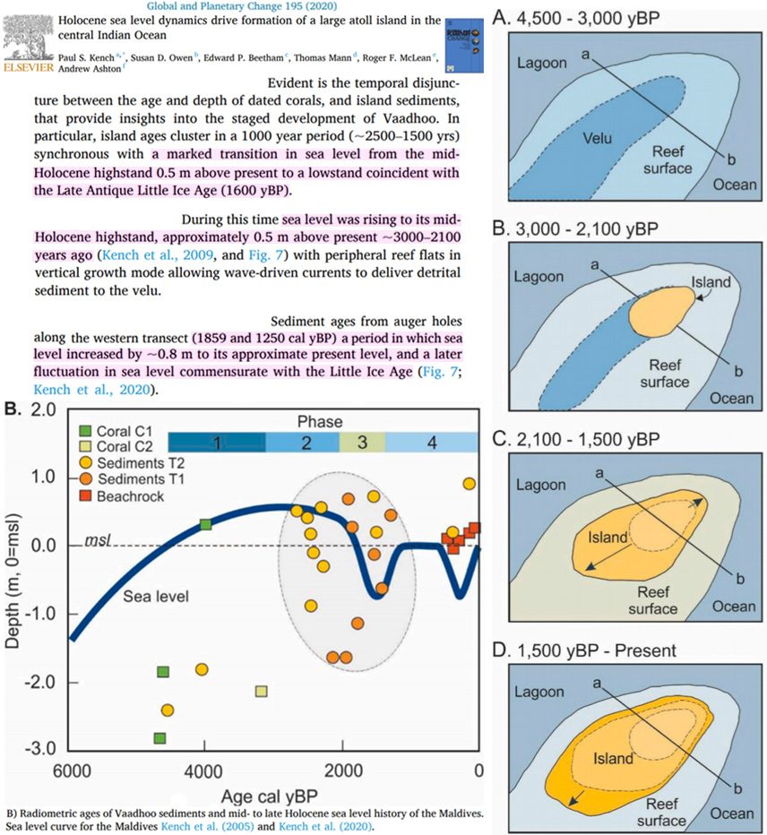
Parker et al., 2020 East Saudi Arabia, +2.8 – 3.75 m higher than present
“The sediments record rapid transgression during the early Holocene with a mid-Holocene high-stand immediately prior to 6880-6560 cal. BP when the upper limit for the palaeo Mean Highest High tide water (MHHW) was 2.8-3.10 m above present day mean sea level. Transgression continued until shortly after 5575-5310 cal. BP with an upper limit to the palaeo-MHHW of 3.75 m above present sea levels.”
Bhattacharya, 2020 Western India, +2 m higher than present
“The Mid-Holocene SL [sea level] that is radiocarbon dated to 7.3 cal yr BP and 5.1 cal BP was ~2 m higher than the present sea level.”
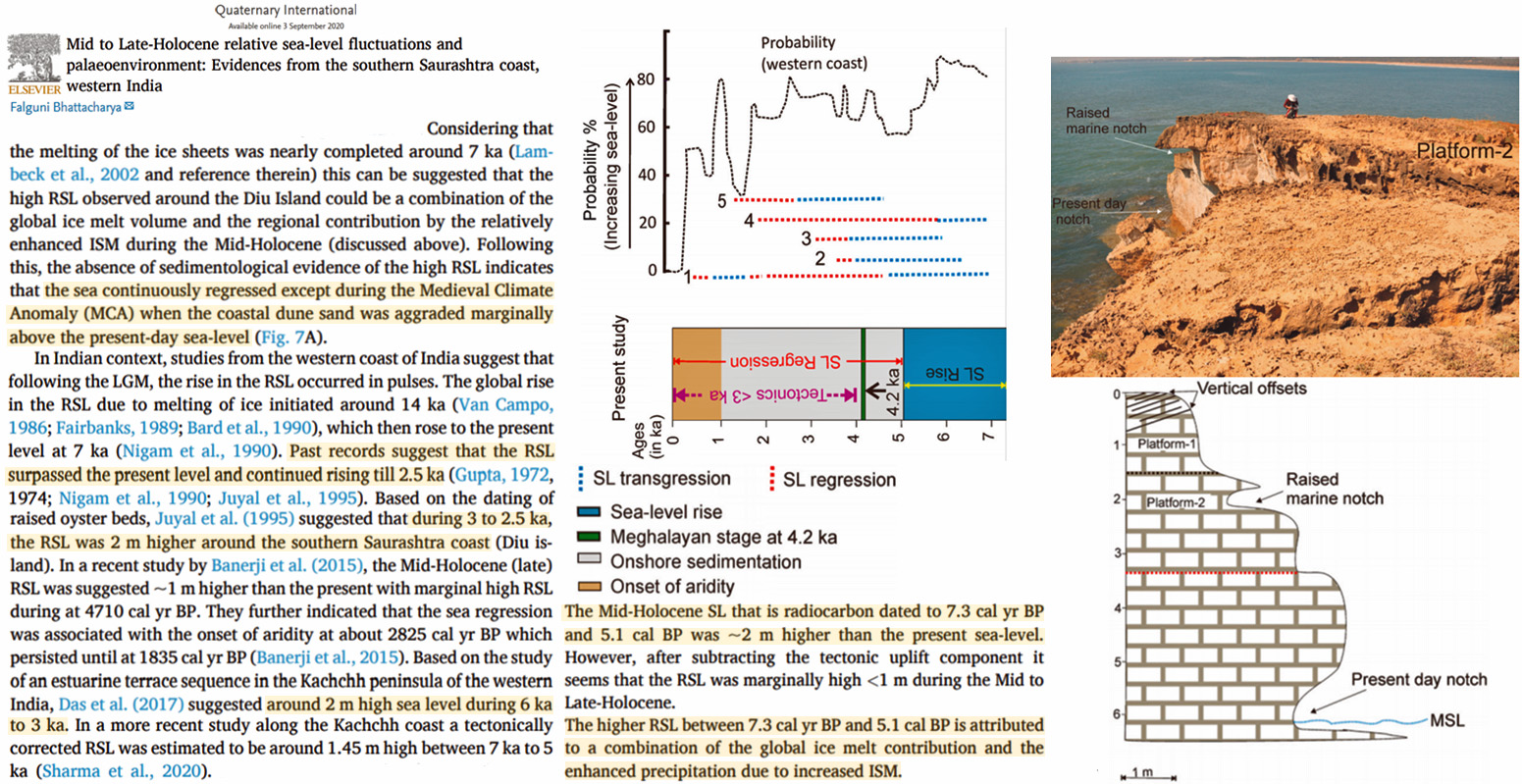
Toniolo et al., 2020 Brazil, +2.9 m higher than present
“In South Brazil, vermetids indicate sea level fall of 2.9 m during the last 4.0 ka. … [T]he last 4.0 cal ka BP, with maximum elevation of + 2.9 m around 4.0 cal ka BP (oldest sample), minimum of + 0.5 m at 0.9 cal ka BP (youngest sample) and average sea level falling velocity of 6.6 cm per century. … The RSL variation curve of São Francisco do Sul (SC) shows smooth fall trend from 2.9 ± 0.5 m at 4.0 cal ka BP until the modern sea level (zero), which is in accordance with the paleo-sea level data obtained from vermetids and compiled by Angulo et al. (2006) for the Brazilian coastal region between 3°S and 28°S (Fig. 6).”
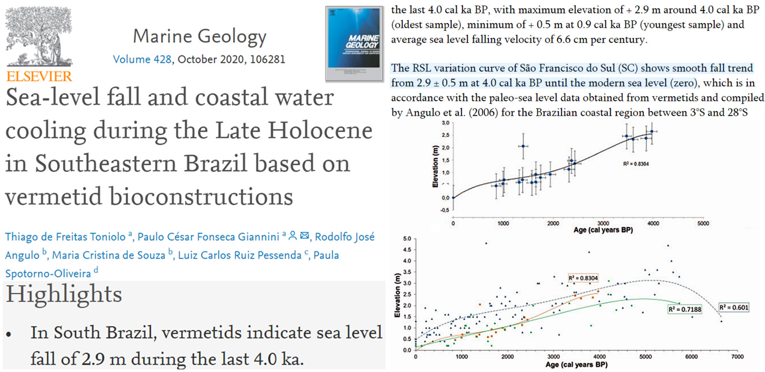
Tanabe, 2020 Japan, +2-3 m higher than present (rate: 40-70 mm/yr)
“During 7-4 ka, the sea level was 2-3 m higher than the present level, and at 3 ka, it fell to -2 m TP. After 2 ka, the sea level stood at the present level. … The following durations, vertical displacements, and rates of sea-level rise have been inferred for MWP1D: 7.6-7.5 ka, 6 m, and 60 mm/yr in the Caribbean Sea (Blanchon et al., 2002) … The rates of three sea-level jumps in Tokyo Bay were >40-70 mm/yr for TB1, >20-50 mm/yr for TB2, and >20-30 mm/yr for TB3.”
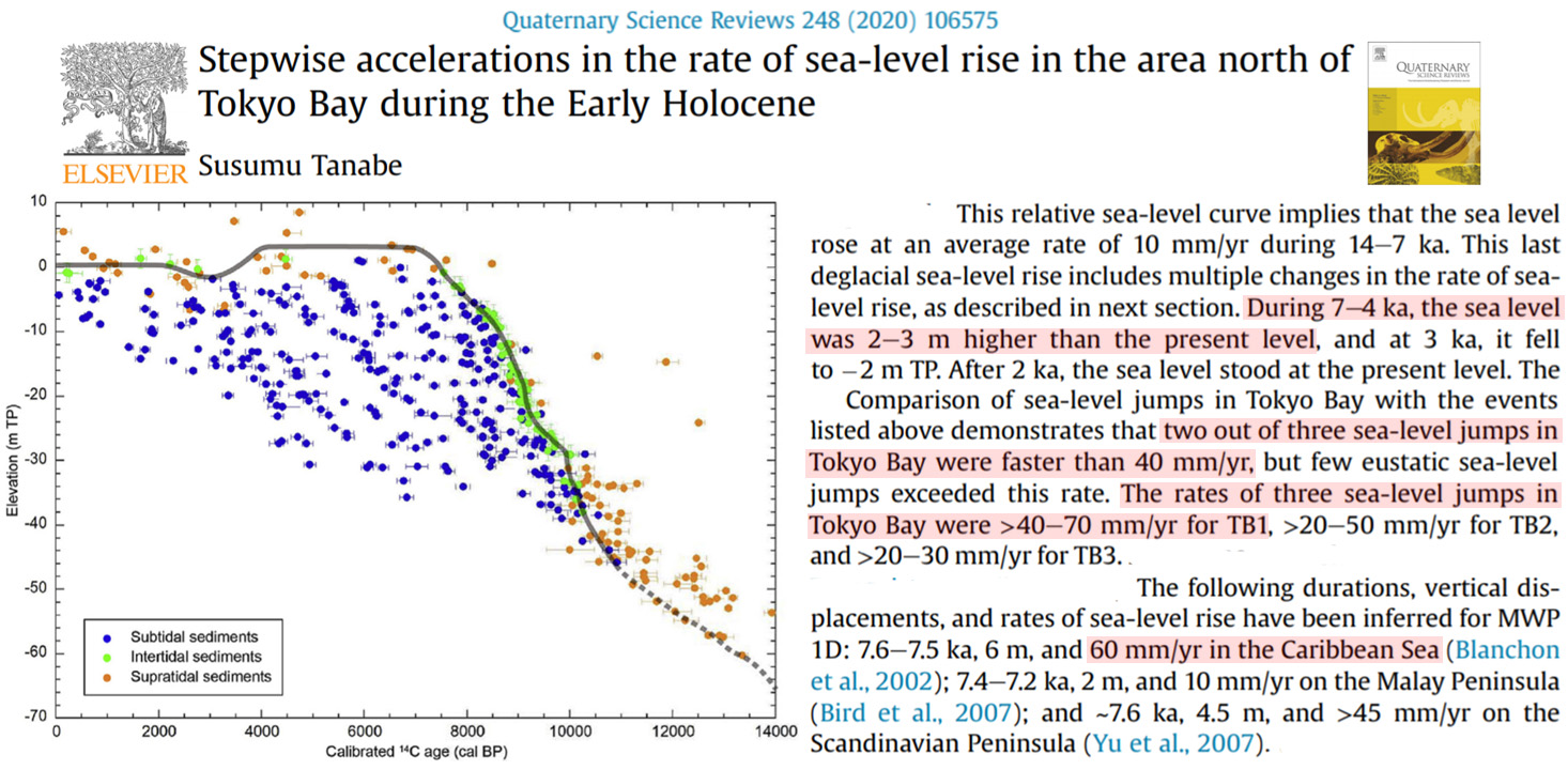
Helm et al., 2020 South Africa, +6 to 8 m higher than present last interglacial
“Around 126 ka, sea levels were 6.6-8 m higher than present levels on the Cape south coast [of South Africa]. … Chronological context11 suggests an age of MIS 5e (the Last Interglacial). As sea levels during MIS 5e in this area were up to 6-8 m higher than at present, a warmer climate capable of supporting large reptiles on the Cape south coast can be inferred.”
Damien et al., 2020 Arabian Gulf, +2.5 m higher than present
“These different trends can be explained by different local conditions. Recent work carried out in northeastern Kuwait estimated a +3.5 m asl [higher than present] highstand (~ 5000–3500 cal. years BP) from beach ridges studied (Reinink-Smith 2015). This highstand is about 2 to 2.5 m higher than the previous maximum identified in the area (Gunatilaka 1986). This new result seems more in line with our data, pushing back the Holocene highstand dating. … [L]andforms associated with this highstand [about 6000 years ago] are today located between 1 and 3 m above the current sea-level.”
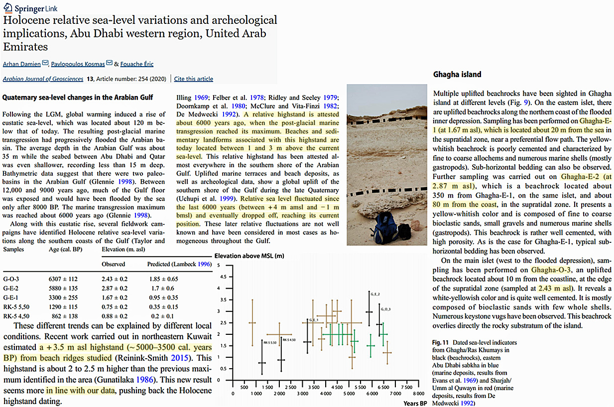
Steffen et al., 2020 Greenland, +32 m above present (13.8 ka)
“The Nanortalik RSL data show rapid early Holocene sea-level fall from at least ∼32 m above present around 13.8 ka cal BP, reaching present-day RSL by c. 10 ka cal BP and continuing to a lowstand in the early Holocene before rising to present in the late Holocene”
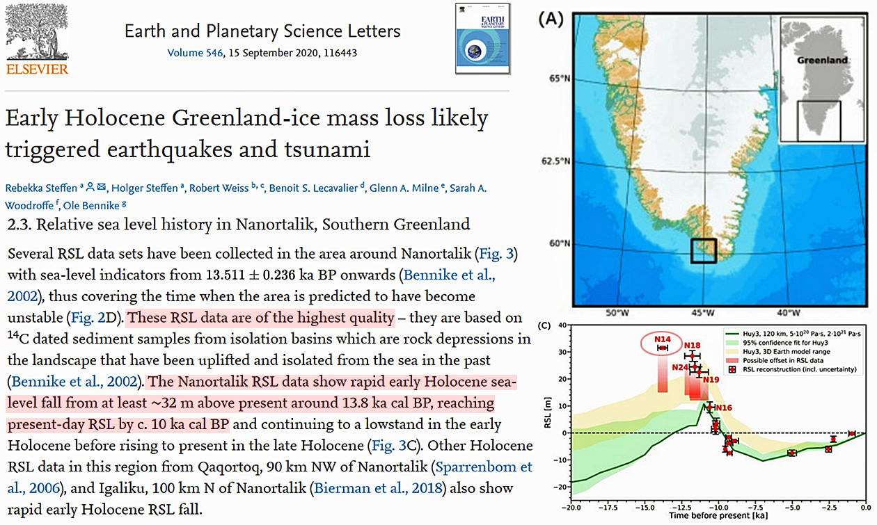
King et al., 2020 New Zealand, +2.65 m above present
“Regional tectonics dominate the relative sea-level signature across much of New Zealand, and trends of uplift and subsidence can vary significantly depending on the timescale of analysis. … Clement et al. (2016) addressed the problem of regional variations in relative sea-level history by integrating a broad selection of mostly published preexisting local sea-level proxy data to generate a series of relative sea-level curves for different parts of New Zealand. … In their study, a highstand in the northernmost North Island was identified from 8.1–7.3 ka BP (0.6–1.4 kyr prior to Gibb (1986) in agreement with Australian records (e.g. Horton et al. 2007; Lewis et al. 2013)), reaching ∼2.65 m above present mean sea level, before falling to present values between 7.8 and 6.4 ka.”
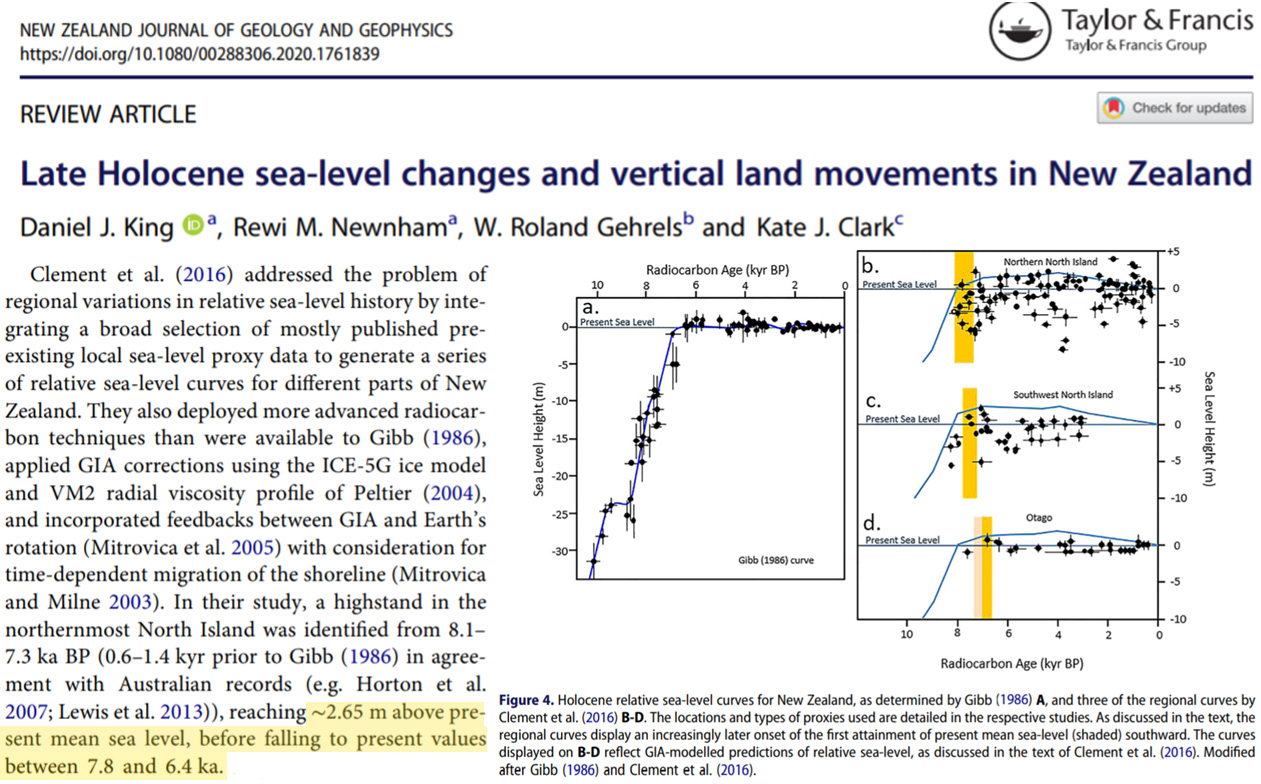
Lopez-Belzunce et al., 2020 Mediterranean, +1-1.2 m higher than present
“Regarding the stabilization of the RSL [relative sea level], our data show it to be 1.20 m above the present-day level at 3000 cal yr BP and 1 m higher at 2000 cal yr BP.”
Areias et al., 2020 Brazil, +4 m higher than present
“At 3700 cal. years BP the RSL was localized at around +4 m above the present sea level, representing the Holocene eustatic maximum for the Rio de Janeiro coast. Estimated SST obtained from the stable isotopes of the aragonitic vermetids was ~20 °C. At ~3300 cal. years BP during the RSL fall the SST reached its upper-Holocene maximum temperature of ~22 °C. At ~2000 cal. years BP, the RSL was +2 m and an intensification of the upwelling events brought about lower SST (~17 °C) in the intertidal/supratidal settings than offshore. … The following period (from ~1900 to ~1300 cal. years BP), characterized by a continuous sea-level fall, recorded a SST of ~20.5 °C, higher than before. … These data show that in the southeastern Brazilian coast the RSL passed from ~ + 4 m at around 3700 cal. years BP to ~ + 1.30 m at 1300 cal. years BP (e.g., Spotorno-Oliveira et al., 2016).”
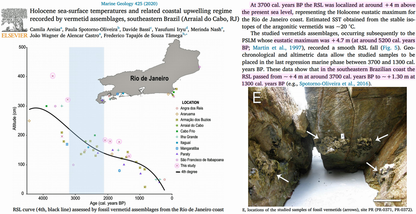
Sissakian et al., 2020 Persian Gulf, +1-2 m above present
“[G]eologists do believe that the Gulf was a dry area and was filled due to melting of huge amounts of ice; accordingly, the shoreline started progressing landwards. After that, due to climate change, the shoreline started retreating downwards due to the delta development of the Tigris, Euphrates and Karun rivers. The present shoreline was reached shortly before 6,000 years ago and exceeded as relative sea level rose (l – 2) m above its present level inundating the low-lying areas of lower Mesopotamia.”
Martins et al., 2020 SE Brazil, +2.4 m above present
“In Armação dos Búzios city, north of Rio de Janeiro State (SE Brazil), Jesus et al. (2017) recognized recently the following evolutionary stages of sea level during the Holocene: a sea-level lower than the current between 8148 and 6300 cal yr BP; a rise in sea level between 6300 and 4500 cal yr BP; a transgressive maximum of about 2.4 m above the present level at 4700–4500 cal yr BP; a sea-level drop from 4500 cal yr BP until the present.”
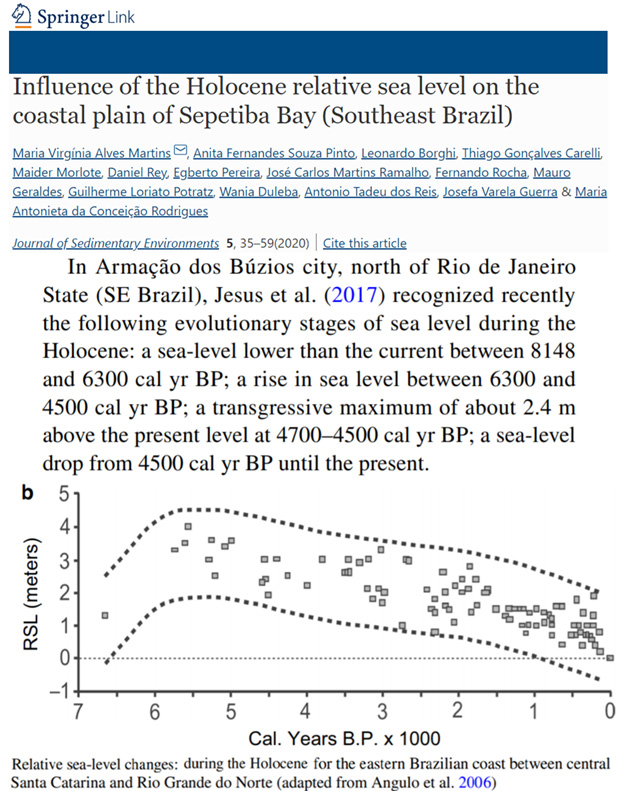
Garrett et al., 2020 Chile, +3-6 m above present
“GIA model predictions display a high degree of variability along the Chilean coastline. The two northernmost regions are characterised by modelled mid Holocene highstands 1.5-5.5 m above present between 7 ka and 4 ka (Fig. 7a and b). The five central regions between Valparaíso and Isla Mocha share modelled highstands 3-6 m above present at 7 ka or 6 ka (Fig. 7ceg).”
Ma et al., 2020 NE China, +2.3 m above present
“The Bachagou Lagoon plain in the south of Changxing Island reached the high sea level of the Holocene about 6000 years ago, which was 2.2 to 2.4 m higher than the present sea level (Fang et al., 2009).”
Clark et al., 2020 Global sea levels +6-9 m above present (Last Interglacial)
“Although the last interglaciation (LIG) experienced stronger boreal summer insolation forcing than the present interglaciation, understanding why LIG global mean sea level may have been six to nine metres higher than today has proven particularly challenging. Extensive areas of polar ice sheets were grounded below sea level during both glacial and interglacial periods, with grounding lines and fringing ice shelves extending onto continental shelves. This suggests that oceanic forcing by subsurface warming may also have contributed to ice-sheet loss analogous to ongoing changes in the Antarctic and Greenland ice sheets. Such forcing would have been especially effective during glacial periods, when the Atlantic Meridional Overturning Circulation (AMOC) experienced large variations on millennial timescales, with a reduction of the AMOC causing subsurface warming throughout much of the Atlantic basin.”
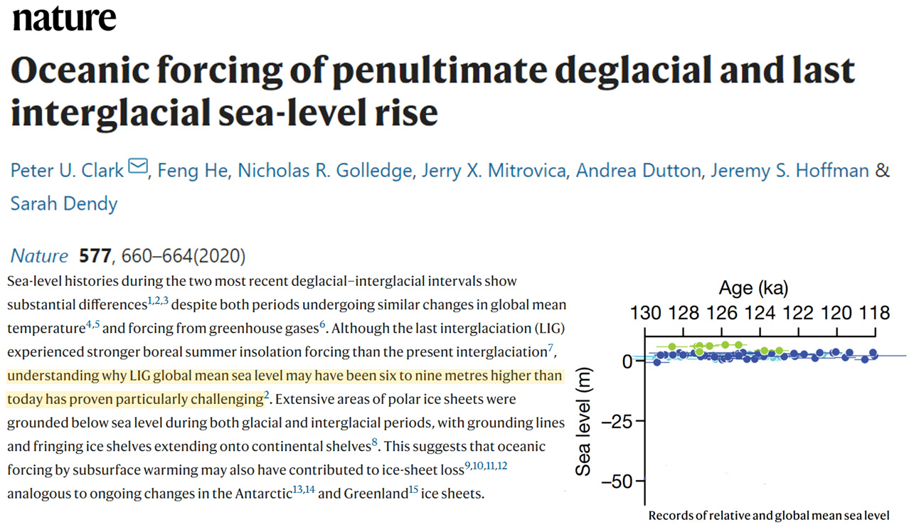
Amato et al., 2020 Italy, current coast still underwater just 300 years ago (0.3 ka)
“During MIS5‐2 shallow marine‐coastal environments turned into fluvial‐marshy environments in response to the last glacial sea‐level fall. At the beginning of the Holocene, rapid sea‐level rise caused a marine transgression that carved a steep cliff >300 m inland (Figure 9a). The MFS, dated at ca. 7.0 ka, was followed by the establishment of an open natural coastal environment that persisted until Roman age. The small sheltered bay of the Fusandola S. paleomouth may have hosted the Roman harbor (Figure 9b). … In 1260 CE, a new harbor with a long quay existed, probably that built by Manfredi di Svevia (Figure 9c). Our chronological and geochemical data evidence the construction of a later new harbor during the 17th–18th centuries, providing independent support to the iconographic evidence from 17th to 18th century CE maps (Figure 9d). During the last century, the harbor structures were covered once again. The latest phase of coastal restoration took place in 2016 CE (Figure 9e).”
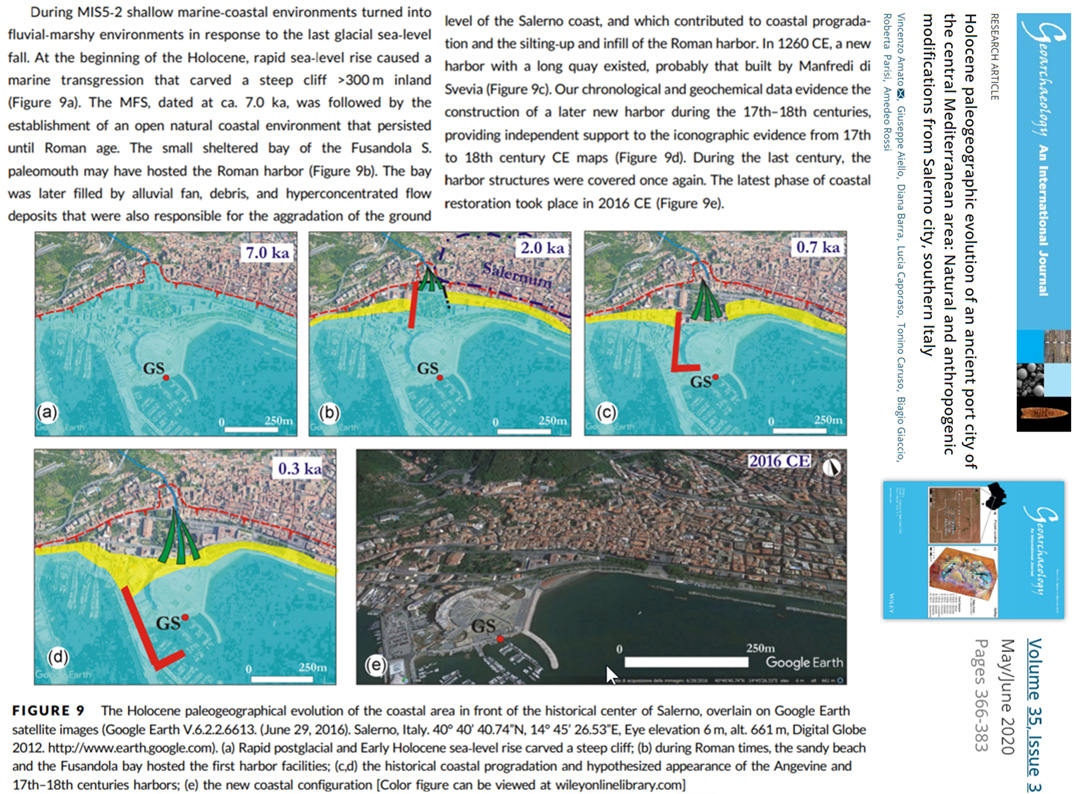
Muh et al., 2020 Bahamas and Bermuda, at least +7 to 9 m higher than present, last interglacial
“Corals with closed-system histories collected from patch reefs on NPI have ages of 128-118 ka and ooids/peloids from beach ridges have closed-system ages of 128-116 ka. Elevations of patch reefs indicate a LIG paleo-sea level of at least ∼7 m to ∼9 m above present. Beach ridge sediments indicate paleo-sea levels of ∼5 m to ∼14 m (assuming subsidence, ∼7 m to ∼16 m) above present during the LIG. …. Results of this study show that at the end of the LIG paleo-sea levels could have been as high as 11-13 m above present (at localities close to North American ice sheets) to as little as 5-8 m above present (at localities distant from North American ice sheets).”
Burley et al., 2020 Polynesia, +1.2-1.4 m higher than present
“At the time of first Lapita arrival at Nukuleka, sea levels were 1.2–1.4 m higher than present (Dickinson 2007).”
Lopes et al., 2020 Brazil, +3 m higher than present
“The late Pleistocene-middle Holocene post-glacial marine transgression (PMT) that started around 18 ka b2k in response to the melting of ice caps and glaciers, together with increased precipitation, would have led to another lake highstand (Figure 3A). Sea-level curves obtained from several sites along the Brazilian coast show that a mean sea level (m.s.l.) equal to the present one was reached at ~7 ka b2k, and continued to rise until reaching up to +5 meters between 6 and 5 ka b2k (Martin et al., 2003; Angulo et al., 2006). In the CPRS the PMT formed the Barrier IV, and the estimates based on geologic and fossil records indicate that it reached amplitude of about 2-3 meters above the present m.s.l. (Barboza and Tomazelli, 2003; Caron, 2007; Lima et al., 2013; Dillenburg et al., 2017).”
“The altitude of the terrace T3 above the fossils of Toxodon found in situ indicates this was cut by the Holocene sea-level highstand that reached a maximum altitude of 3 meters [above present] between 6 and 5.1 ka b2k. At that time Mirim Lake was invaded by the Atlantic Ocean through Taim and São Gonçalo channel, becoming a large paleo-lagoon with conditions suitable for its occupation by marine organisms, including sharks, rays, teleost fishes and whales. The coastal waters were warmer than today, as indicated by the presence of fossils of the shark Carcharhinus leucas, common in tropical areas.”
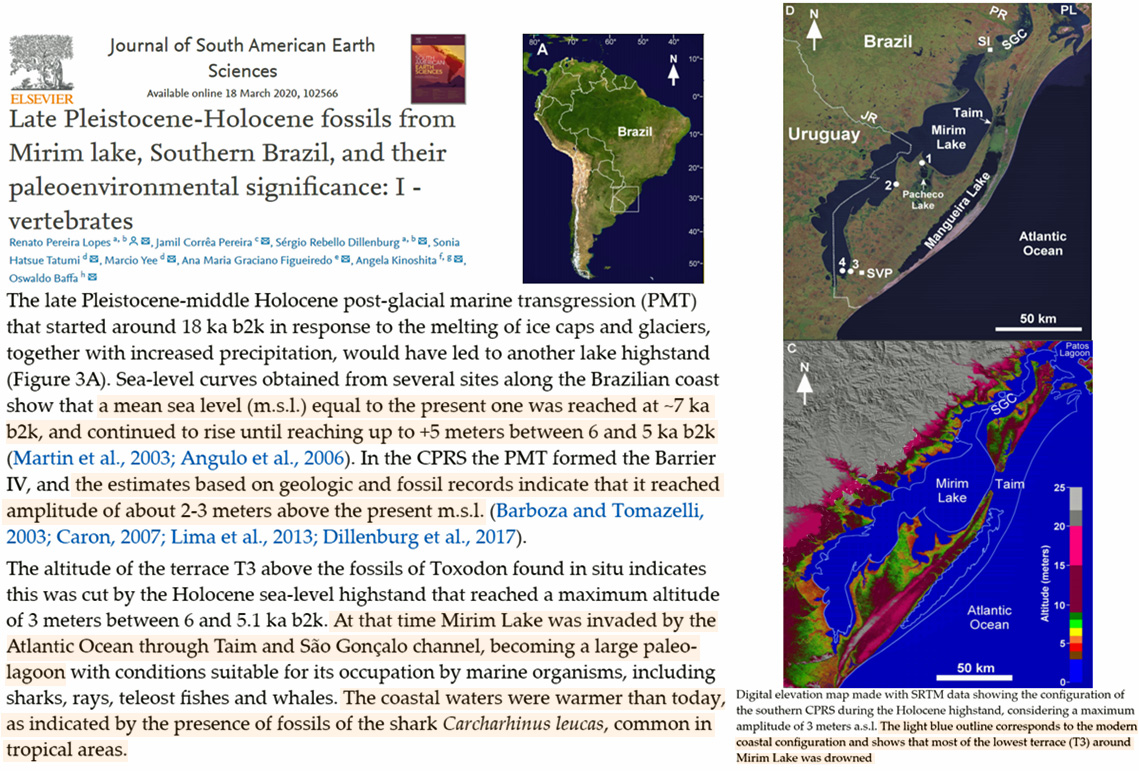
Brocx and Semeniuk, 2020 Western Australia, +1 m higher than present
“The Holocene stratigraphy in the Walpole–Nornalup Inlet Estuary shows that mean sea level was 1 m higher than present some 2900–1200 years BP (Semeniuk et al., 2011).”
Helfensdorfer, 2020 Australia, +2 m higher than present
“This study presents a well-constrained model of the geomorphic evolution of the lower Murray River and Murray estuary with a specific focus on the response of the system to the Holocene sea-level highstand. Hydrodynamic modelling of the lower Murray River and Murray estuary was conducted to evaluate the primary drivers of palaeo-environmental change during the Holocene and constrain the plausible response of the Murray estuary to the +2 m higher-than-present sea level of the Holocene sea-level highstand.”
Martin et al., 2020 Western Australia, +2 m higher than present
“Sea level high stands (~2 m higher than present) occurred at ~7 and 4 ka (Gouramanis et al., 2012) that likely caused seawater intrusion events into the aquifer”
Glaciers, Sea Ice, Ice Sheets
Our results are consistent with previous literature demonstrating a SW warming response to reduced Greenland cloud cover particularly in ablation regions and for the area-averaged ice sheet (Box et al., 2012; Hofer et al., 2017; Lim et al., 2016; Wang et al., 2018, 2019), as well as with studies finding LW warming effects of enhanced cloud cover over accumulation regions (Bennartz et al., 2013; Miller et al., 2015; Wang et al., 2018, 2019). … Declining cloud cover since the mid-1990s allowed more shortwave radiation to reach the ice sheet surface (Hofer et al., 2017), promoting a surface SWD increase of 7.3 W/m2 from 1994 to 2017 for the control experiment (R2 = 0.29, P = 0.007; Figure 6c,e), in contrast with reduced SWD in the flat experiment. SWD enhancement for the control run is strongest and most significant for southern Greenland (Figure 10e), corresponding to the strongest cloud cover reductions (Figure 10d). … Consistent with these studies, we find that increased cloud cover under blocking conditions drives dominant LW warming over high albedo, high elevation regions of the GrIS. In contrast, reduced cloud cover drives dominant SW warming over low albedo, low elevation regions under blocking conditions. Additional clear sky LW warming counteracts cloud-driven LW cooling over southern and peripheral Greenland to produce all sky LW warming over the entire ice sheet. SW warming in the ablation zone currently dominates the melt signal, as warm mean state temperatures allow energy anomalies to produce melting, while LW warming in the colder accumulation zone largely contributes to snowpack heating.
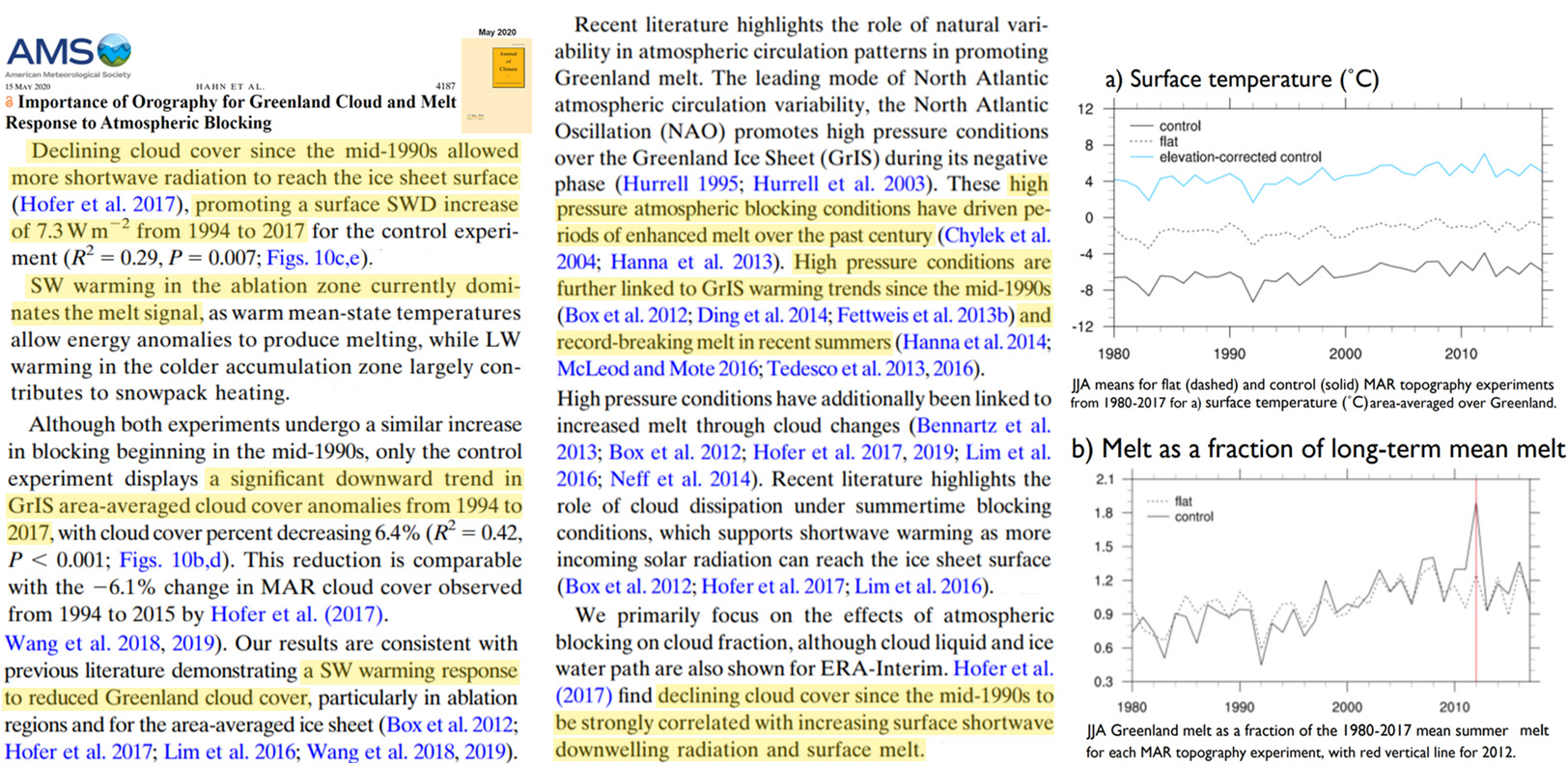
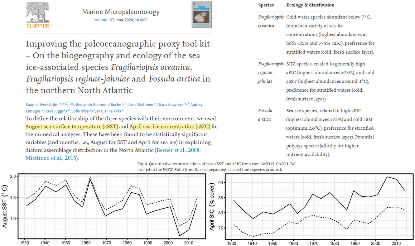
The LIA was the coldest period during the Holocene, when most of the glaciers reached their largest extent since the end of the Pleistocene (Svendsen and Mangerud, 1992; Mangerud and Landvik, 2007: Miller et al., 2010). A similar scenario was described for other sites, e.g. south Hornsund (Wójcik and Ziaja, 1993), Treskelen (Birkenmajer and Olsson, 1997; Philipps et al., 2017), and Scottbreen (Mangerud and Landvik, 2007). The dating of the shells, found in marginal moraine, eskers, and the dirt cones at Werenskioldbreen, indicates that the ice reached lesser extents before 12.1 cal ka BP than today (Birkenmajer and Olsson, 1998; Hormes et al., 2013). … These data suggest that the ice load at the Last Glacial Maximum (18 ka BP) in North Hornsund was the lowest compared to surrounding areas (Chmal, 1987). In contrast, driftwood dated to almost 10 ka BP was found at 100 m elevation on Kongsøya (Salvigsen, 1981).
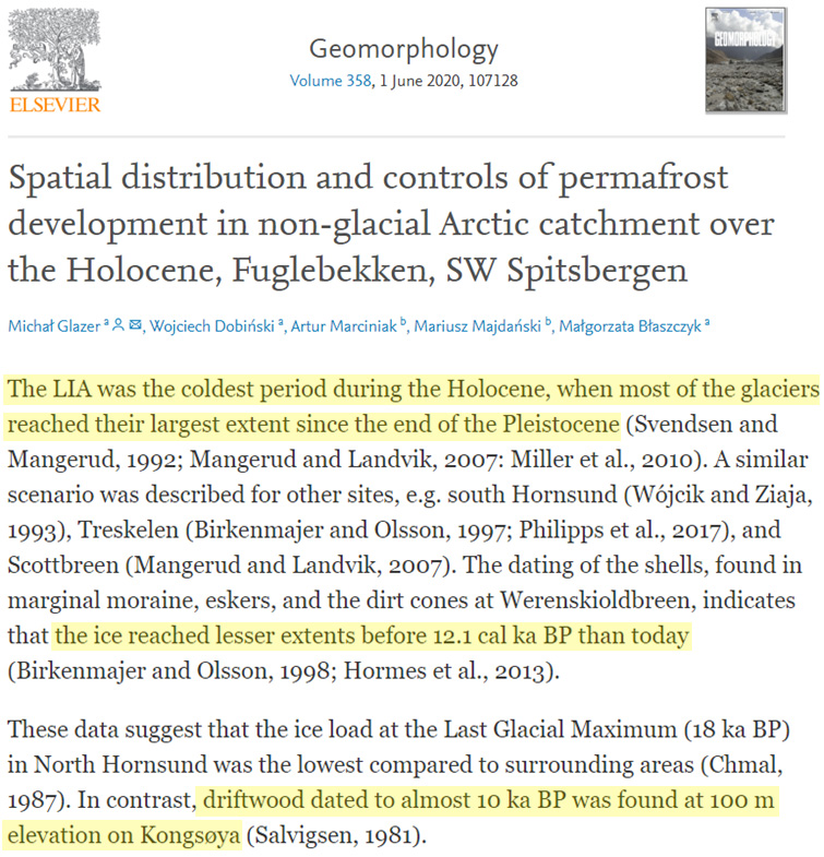
The conditions in northern Spitsbergen are thus comparable to central western Spitsbergen during the Early to Middle Holocene, where some of the smaller ice caps disappeared and tidewater glaciers retreated to positions several kilometres farther back than their modern margins (Mangerud & Svendsen 1990; Svendsen & Mangerud 1997; Hald et al. 2004; Forwick & Vorren 2009; Baeten et al. 2010). … In Wijdefjorden the few modern tidewater glaciers are located tens of kilometres (up to 100 km) away from the study area (Fig. 1C). The very low sediment accumulation rate after 7.1±1.0 cal. ka BP could indicate a Holocene glacier minimum in the Wijdefjorden area (Figs 7, 10C), where glaciers had retreated onto land and innermost fjord positions. … The almost synchronous increase in IP25 concentrations after c. 0.7±0.2 cal. ka BP, with a maximum in the modern sediments, indicates more sea ice towards the Late Holocene.
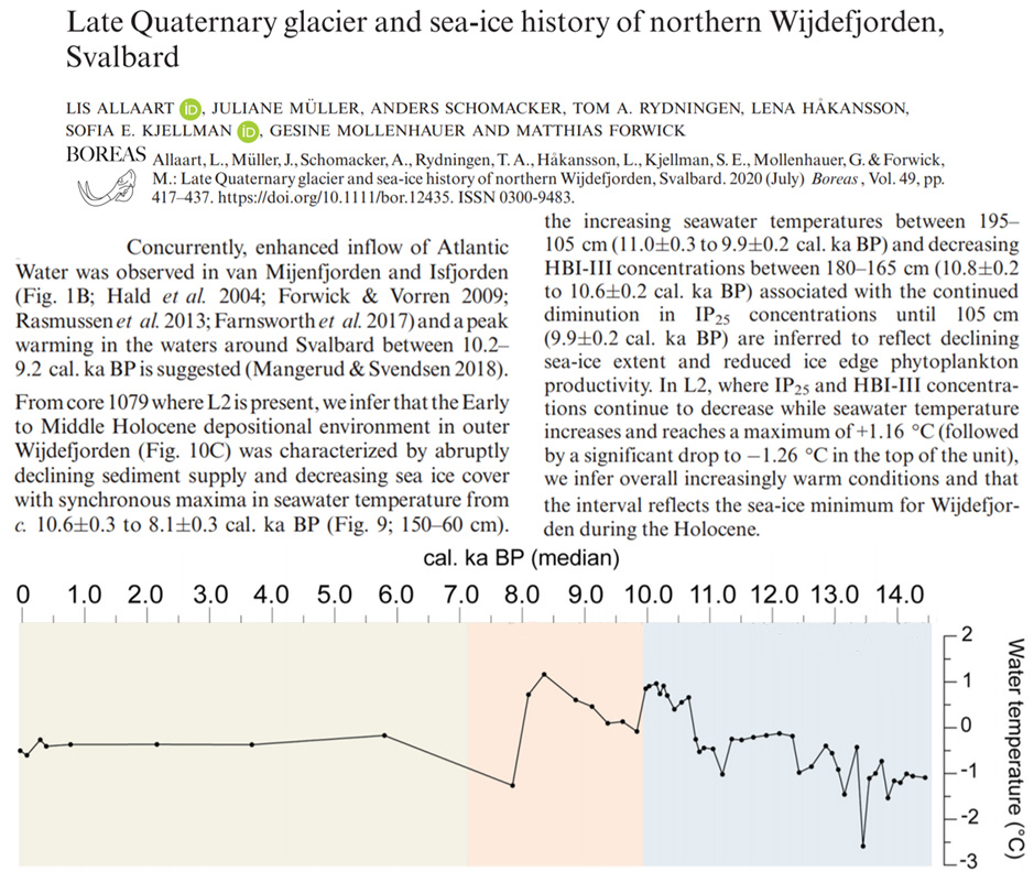
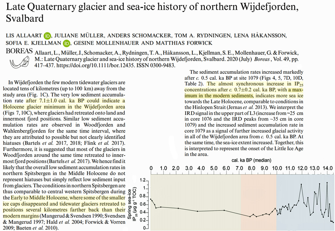
In the early Holocene, i.e., prior to the first HBI-III peak, it was nearly ice free throughout the year, reflected in very low PIP25 values < 0.2 and variable SSTs (Fig. 7a, c). Then, a general trend toward an increasing sea-ice cover is coinciding with weakened insolation. … Higher values of HBI TR25 may point to enhanced occurrence of spring blooms between 8 and 5 kyr BP, indicating that the core site was relatively ice free in spring. … During the early Holocene … both the foraminifera study and our biomarker records (Fig. 7c) display more open-water conditions in comparison to the modern Beaufort Sea. … During the deglaciation and the early Holocene (~14–8 kyr BP), minimum concentrations of IP25 (close to the detection limit) and low PIP25 values point to dominantly ice-free conditions.
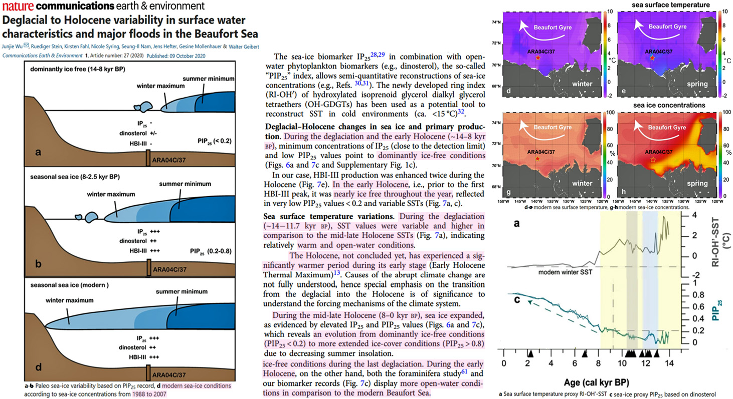
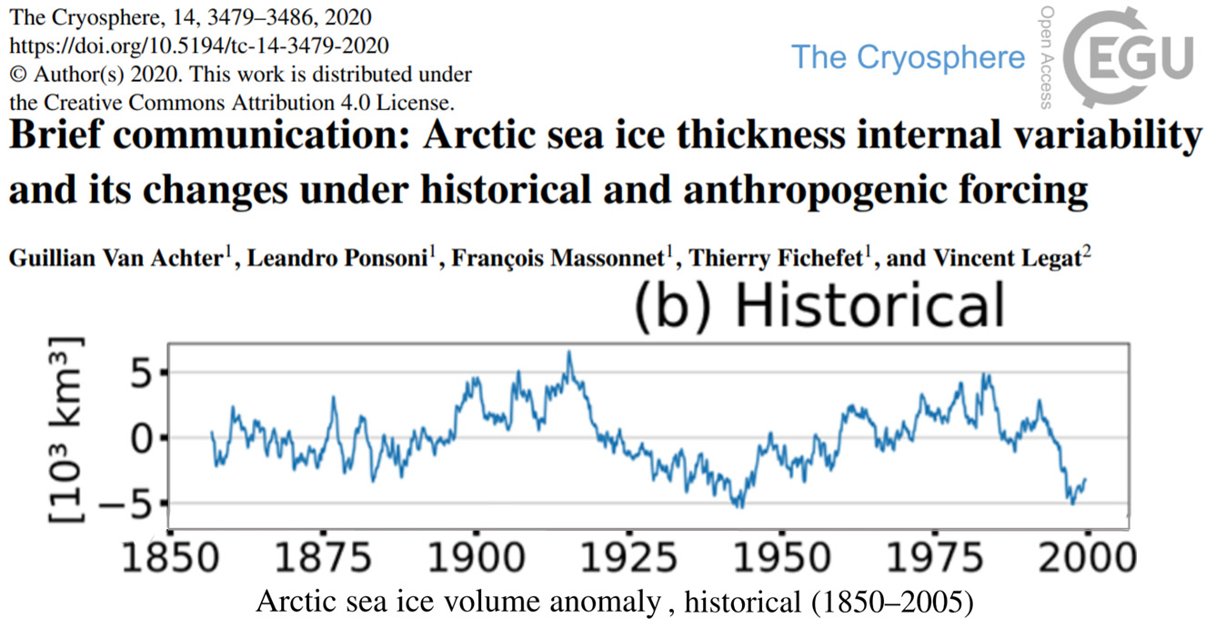
[O]ur PIP25 indices show relatively moderate values (0.2–0.6), suggesting a reduced sea ice cover, especially between about 2.4 and 1.0 ka BP (Fig. 5a). Sea ice might have only occurred during the late winter/early spring of this time span, as shown by minimum PIIIIP25 values and the HBI III maxima (Figs. 4c, 5a). Notably, the pronounced peaks in HBI III fux and TR25 (Fig. 5b) at about 2.1 and 1.3 ka BP that might coincide with the Roman Warm Period (RWP) and Medieval Climate Anomaly (MCA), respectively, can be associated with stronger WGC pulses.
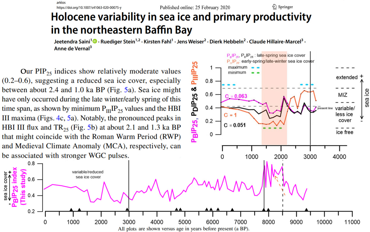
The contrasting hydroclimatic changes in the Karakoram region and the western Himalaya, as inferred from the glacier mass balance data, are based on the observations of the past few decades. However, our study shows the persistence of contrasting hydroclimatic variability over the past millennium (Figure 3d and 3e), which indicates that the ‘Karakoram anomaly’ is part of natural variability. … This study indicates that the ‘Karakoram anomaly’ is a natural phenomenon and is probably caused by spatially varying hydroclimatic trends in HMA.
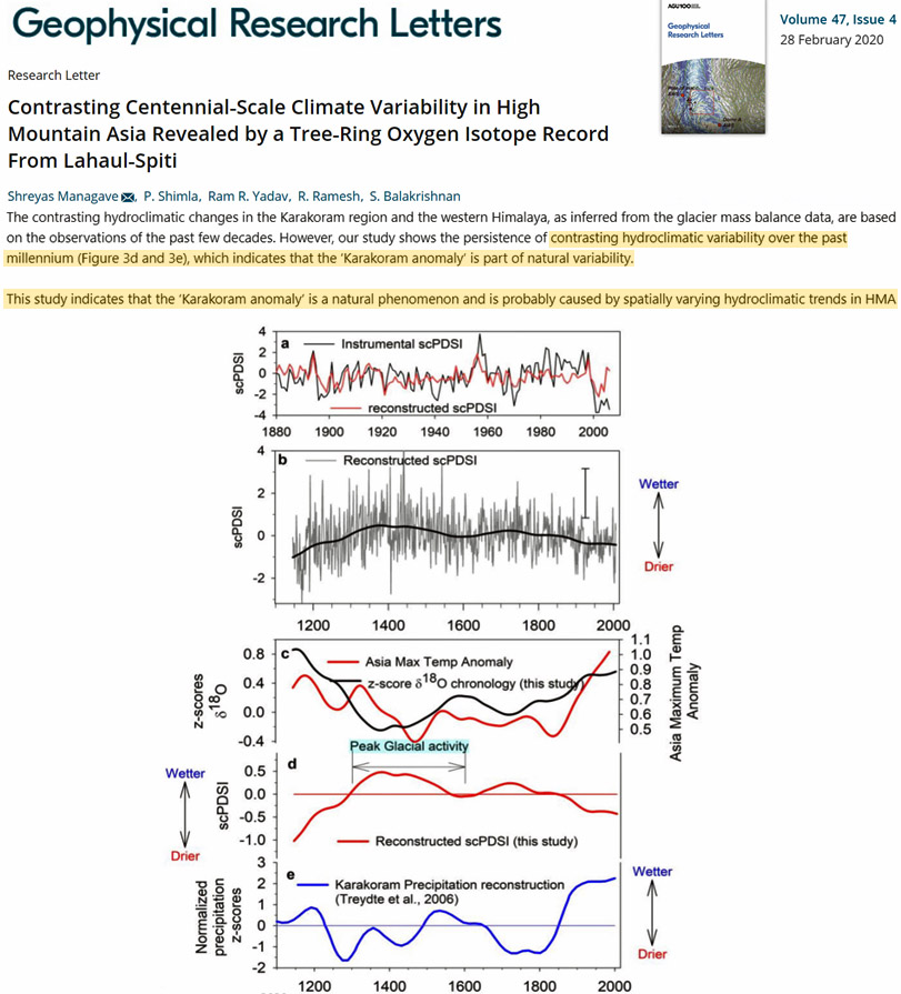
Even though the global retreat of glaciers since 1850 is considered to be a fingerprint of man’s influence on the climate, it is now evident that considerable glacial fluctuations occurred already much earlier during the Holocene, when human impact was negligible. … Such small CO2 variations are unlikely to trigger the observed glacier movements. It is therefore possible that small solar activity variations [23], enhanced by (hitherto largely unknown) feed-back processes on Earth caused the observed glacial fluctuations [24]. … Surprisingly, up to 10,000-year old logs were found in the forefield of the Pasterze glacier, the largest glacier in the Austrian Alps [10], The situation of the finds is depicted in Fig. 2. This indicated that in the Early Holocene these glaciers were even smaller than today, allowing trees to grow in an area still covered by ice today. … The longest exposure times (4.5 to 5.3 kyr) were found at the left-lateral margin zone of the [Rhone] glacier indicating the longest integral time when the glacier was smaller than today.
With this slowdown, the terminus region transitioned from net annual thinning to net annual thickening (Khazendar et al., 2019). This slowdown coincided with a period of increased surface mass balance and cooler atmospheric and ocean temperatures (Joughin et al., 2018; Khazendar et al., 2019; Mouginot et al., 2019). … The record is sparser for 2016, but it is sufficient to indicate that increased thickening occurred during the winter of 2016–2017 as the ice tongue advanced and the glacier slowed. As a result, just prior to the summer speedup in 2017, the terminus region was ∼ 35 m higher than the previous summer (see also Khazendar et al., 2019). Winter thickening continued to outpace summer thinning so that by March 2019 surface elevations near the terminus were only 10 to 20 m lower than those observed during spring of 2011 (Fig. 2b). … The time series of elevation provides an unprecedented level of detail, which clearly shows a pattern of summer thinning partially offset by winter thickening in response to seasonal changes in flow speed over most of the record. At least from autumn 2016 through spring 2019, winter thickening outpaced summer thinning, leading to net thickening and elevations approaching those observed in 2010.
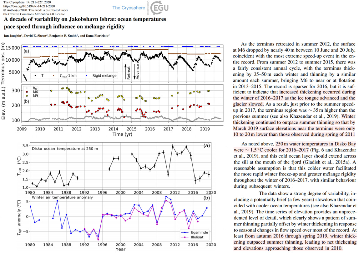
Recent winters have been unique due to the rapid and extreme cooling of the subpolar North Atlantic. Here, we present a novel view on its causes and consequences. Combining in‐situ observations with remote sensing and atmospheric reanalysis data, we show that increased freshening of the subpolar region gives rise to a faster surface cooling in fall and winter. Large freshwater events, in particular, result in pronounced cold anomalies with sharp temperature gradients that promote an enhanced storminess. The storms reinforce the cooling by driving stronger heat losses and modulating the surface flow. Consistent with this mechanism, past freshwater events have been followed by cold anomalies in winter of ~‐2°C and increases in the North Atlantic Oscillation index of up to~0.6 within 3 years. We expect that future freshwater discharges into the North Atlantic will amplify the cold anomaly and trigger an enhanced wintertime storminess with far‐reaching climatic implications.
Our results demonstrate that abrupt ice loss of several hundred meters occurred at a similar rate and duration across multiple outlet glaciers in the Mid-Holocene, despite complex bed topography. This implies a common, most likely ocean-temperature, forcing of ice sheet retreat at this time. … The exposure ages at Mawson Glacier decrease with elevation and are concentrated to between ca. 8 and ca. 4.5 ka at both elevation transects (Fig. 2; Fig. S3). During this time period, 22 samples record 220 m of ice surface lowering at Bruce Point, and eight samples record 125 m of lowering at Mount Murray, ∼10 km farther up-glacier. Linear regression analysis indicates that this thinning event started at least by 7.3–6.4 ka (2σ) and continued for ∼705 yr at a best-fit rate of 35 cm yr−1 (21–437 cm yr−1, 2σ) at Bruce Point, and by 6.1–5.4 ka for ∼515 yr at a best-fit rate of 26 cm yr−1 (10–416 cm yr−1, 2σ) at Mount Murray (Figs. S5 and S6). Thinning of the glacier likely initiated before these times, and we cannot rule out that ice surface lowering continued below the present-day glacier surface. … Grounding-line retreat and corresponding ice drawdown in the western Ross Sea then became more gradual during the Mid- to Late Holocene, similar to that recorded in parts of the southern Transantarctic Mountains (Spector et al., 2017), reaching a near-modern ice geometry within the last millennium. … [C]omplex bed topography should result in outlets retreating independently of each other, and, therefore, the consistent timing of abrupt thinning implies an overarching external driver of retreat.
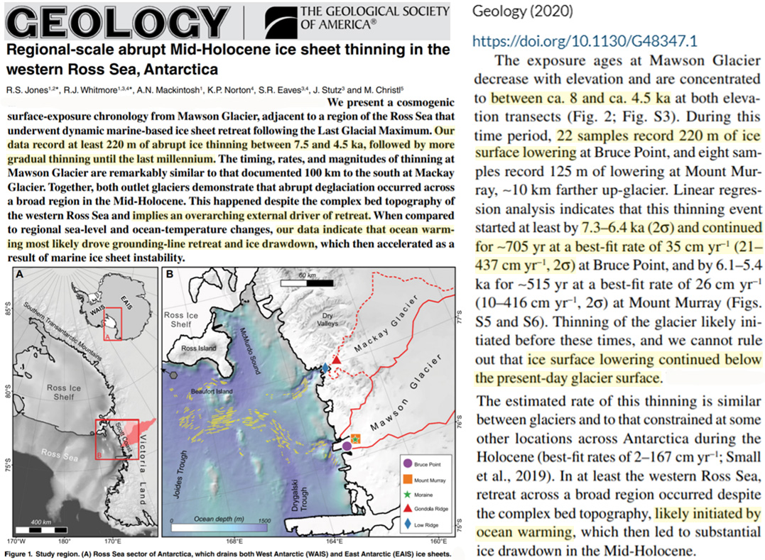
We bring together new and previously published data that relates to Greenland ice sheet change to calculate how quickly the ice sheet retreated between 12,000 years ago and the present. Using this information, we determined that the warmest time of the past 12,000 years occurred between about 10,400 and 9,100 years ago, which is several thousand years earlier than some previous estimates.
After the ice margin reached its present-day position it continued to retreat farther inland. Wood fragments in front of the Hiawatha Glacier demonstrate that the land-based part of the GrIS in Inglefield Land was smaller than present between ca. 5.8 and 1.9 ka cal BP. In addition, the age distribution of the molluscs collected at the Humboldt Glacier margin indicates that the glacier was behind its present-day position between ca. 3.6 to 0.5 ka cal BP (Fig. 7a). At the northern flank of Humboldt Glacier, radiocarbon ages of reworked marine molluscs suggest that the glacier retreated at least 25 km farther inland between ca. 3.7 and 0.3 ka cal BP (Bennike, 2002), possibly favoured by the bed topography being below sea level tens of kilometres inland (Morlighem et al., 2014, 2017). Thus, no later than ca. 0.3 ka cal BP, the GrIS in Inglefield Land re-advanced towards its LIA maximum extent. … At Upernavik and in Melville Bay, the ice sheet was behind its present-day position between ca. 9.1 and 0.4 ka cal BP (Bennike, 2008; Briner et al., 2013; Briner et al., 2014; Axford et al., 2019; Søndergaard et al., 2020) (Fig. 8c). Farther north, mosses from a local ice cap and subfossil plants from the GrIS show a smaller than present-day extent before ca. 3.3 ka cal BP around Qaanaaq and throughout most of the Holocene until ca. 1850 AD in the Thule area (Farnsworth et al., 2018; Axford et al., 2019; Søndergaard et al., 2019).
“Absence of older ice on the highest glacier of South Tyrol is consistent with the removal of basal ice from bedrock during the Northern Hemisphere Climatic Optimum (6-9 kyrs BP), the warmest interval in the European Alps during the Holocene” [36]. Consequently, the measured cosmogenic nuclide concentration in the sampled material integrates the periods when these rocks were ice-free during the Holocene. … Overall, the mean temperature went through a maximum during the first half of the Holocene, sometimes called the Holocene Thermal Maximum (HTM), and continuously decreased in the second half of the Holocene approaching its lowest values during the Little Ice Age (LIA) between 1300 and 1850 AD. This period also resulted in the largest glacier advance during the Holocene …The longest exposure times (4.5 to 5.3 kyr) were found at the left-lateral margin zone of the glacier indicating the longest integral time when the glacier was smaller than today.
At ~7.1 and ~7.3 ka BP, the Quvnerit and Alakariqssoq records show a nearly synchronous shift to organic, non-glacial sedimentation recording the disappearance of local glaciers, while Uunartoq’s glaciers disappeared prior to ~5.2 ka BP. We infer from reconstructed DELAs that summer temperatures were at least 1.2-1.8°C warmer than present by ~7.3-7.1 ka BP. Our records are in good agreement with other studies which suggest that southern Greenland and the Labrador Sea region experienced a delayed thermal maximum (relative to summer insolation forcing and to climate at sites farther north). GIC records from across Greenland show a corresponding latitudinal trend, with local glaciers in northern Greenland becoming smaller than their current sizes or disappearing earlier in the Holocene than those in the south.
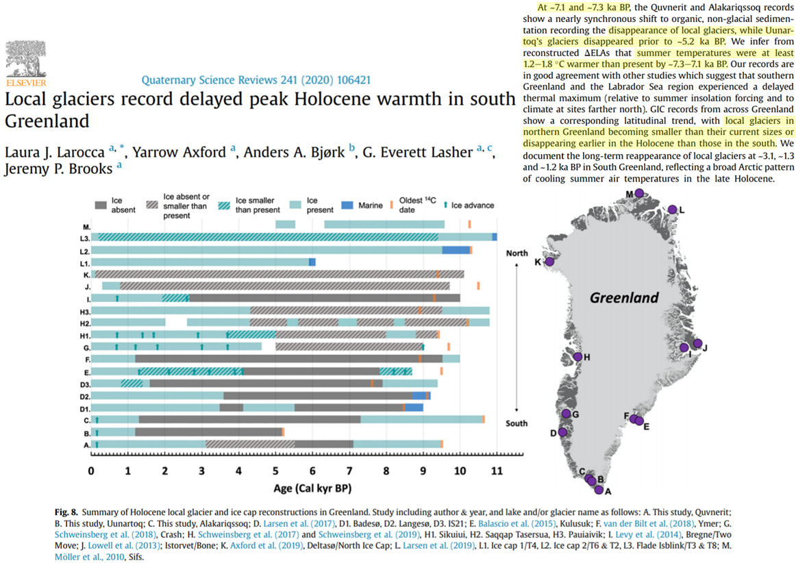
Low Antarctic continental climate sensitivity due to high ice sheet orography … The Antarctic continent has not warmed in the last seven decades, despite a monotonic increase in the atmospheric concentration of greenhouse gases.
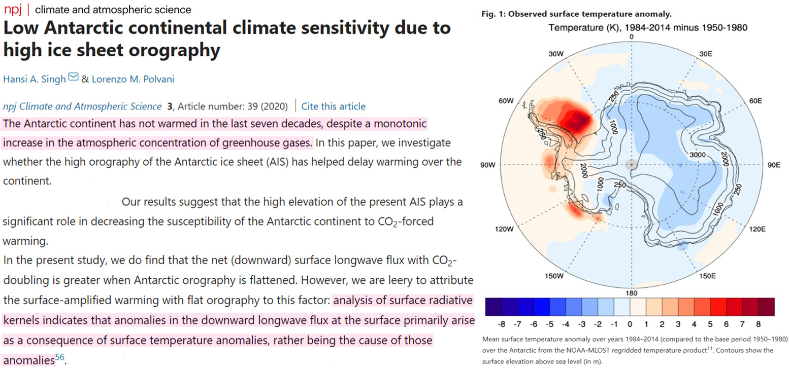
A major outcome of this analysis is that most of the glaciers that have surged recently, have also surged in the 1950 to 1960s as surge cycles are often in the 40 to 60 year range. Combined with further evidence of previous surges, it seems that the so-called ‘Karakoram Anomaly’ is around since at least 200 years. It is also shown that two glaciers that are listed as surging are only expanding, that flow blocking of tributaries plays an important role for several surges, that surging glaciers are mostly free of debris, and that surges show a great variability in regard to surge durations (from 2 to 50+ years) and surge cycles (from 20 to 80+ years).
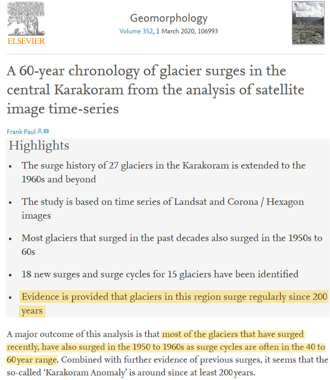
Dynamic response of the Greenland ice sheet to recent cooling … From 2013 to 2019 however, we observe an acceleration in ice motion coincident with atmospheric cooling and a ~15% reduction in mean surface melt production relative to 2003–2012. … Since the record surface melt in 2012, a period of relative stability in mass balance has been observed across Greenland, with 2017 having the lowest maximum surface melt extent since 1996. This stability is coincident with positive Arctic and North Atlantic Oscillations, promoting cyclonic conditions thereby reducing incoming solar radiation and enhancing precipitation.
Amery ice shelf extent is prograding [expanding] considerably in the last two decades. … The study reveals that the AIS extent has been prograded at the rate of 994 m/year with an average 14.5 km increase in the areal extents during 2001–2016, as compared to the year 2001, whereas, the maximum advancement in ice shelf extent was recorded during the 2006–2016 period.
In 2017–2019 a surge of Shispare Glacier, a former tributary of the once larger Hasanabad Glacier (Hunza region), dammed the proglacial river of Muchuhar Glacier, which formed an ice-dammed lake and generated a small Glacial Lake Outburst Flood (GLOF). Surge movement produced the highest recorded Karakoram glacier surface flow rate using feature tracking (~18 ± 0.5 m d−1) and resulted in a glacier frontal advance of 1495 ± 47 m. The surge speed was less than reports of earlier Hasanabad advances during 1892/93 (9.3 km) and 1903 (9.7 km). Surges also occurred in 1973 and 2000–2001.
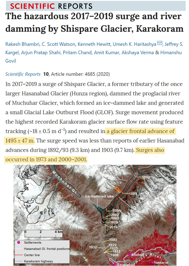
A minimum of seven glaciers at Mt. Xinqingfeng and Mt. Malan showed heterogeneous variations with either surging or advancing during the observation period. Among them, the West Monuomaha Glacier, Monuomaha Glacier, and Zu Glacier were identified as surging glaciers, and the others may also be surging glaciers, although more evidence is required. These glaciers showed a long active period and low velocities. Therefore, we suggested that thermal controls are important for surge initiation and recession. … Glaciers in the eastern and southern ITP have shown significant retreating and mass loss, which is similar to that seen at the Himalayas and Nyainqentanglha, and is influenced by the weakening Indian monsoon [2,14]. However, as observed for West Kunlun, glaciers in the western ITP have remained stable or shown a slight mass gain and are influenced by strengthening westerlies [2,14]. … Several studies have reported that glaciers at Kangzhag Ri and Purogangri experienced near stable mass (−0.04 ± 0.02 m w.e. a−1) and mass gain (+0.16 ±0.02 m w.e. a−1) during 1999–2012, respectively [15,16]. … Based on a 107.07 m ice core recorded from the Malan Ice Cap in May 1999, there has been a warming trend during the 20th century and the warmest period recorded was during the 1950s to the early 1980s. … The glaciers showed heterogeneous variations with some advancing or surging (Tables S1 and S2). Overall, the shrinkage speed of the glacier area decreased after 2000, and the glacier area was stable after 2013, which can be mainly attributed to heterogeneous variations, with some of the glaciers advancing or surging (Tables S1 and S2).
After the end of the LGM initial deglaciation of land areas in Antarctica took place between 10,000 and 8000 yr BP and prosecuted gradually until 5000 yr BP (e.g., Ingolfsson et al., 1998). Mid-Holocene glacial re-advances were recorded from various sites around Antarctica, with intervals of climate warmer than today 4700–2000 yr. Records from the Antarctic Peninsula and coastal Victoria Land suggest climatic optimums from 4000 to 3000 and 3600 to 2600 yr BP, respectively, followed by Neoglacial re-advances (e.g., Ingolfsson et al., 1998). … Based on new radiocarbon dates, during the MWP, the rate of glacier retreat was 1.6m yr1, which is comparable with recently observed rates (Guglielmin et al., 2016).. … Since the second half of the twentieth century, climate warming has been detected in the Antarctic Peninsula with evident impacts on ecosystems (e.g., Cannone et al., 2016). However, a cooling trend of -0.47°C/decade from 1999 to 2014 was recorded in the Antarctic Peninsula, triggering rapid vegetation responses (Sancho et al., 2017).
We compare the cliff morphology of the mid-1950s and the mid-1960s with various time-steps between 1985 and 2017. The studied ice margin remained remarkably constant with very subtle changes of changing sign: rather slow advance rates are reported from the 1950s and 1960s that accelerated until 1985 and were followed by a general retreat until 2012 and a subsequent advance until 2017. Thickness changes are negative throughout the entire time-period, however, different rates of thinning are shown and there is a positive relationship with air temperature anomalies. Compared to similar elevations on the adjacent Greenland ice sheet, we find significantly weaker thinning rates at the NIC.
Of the ∼27 000 glaciers in the Alaska region (including neighboring Canada; Keinholz and others, 2015), four have continuous mass balance records exceeding 50 years in length. Taku and Lemon Creek Glaciers present the longest records in North America, measured annually since the mid-1940s and early 1950s. Despite the close proximity (∼30 km) of these glaciers (Fig. 1), their mass balance histories have diverged. During the past 70 years, Taku Glacier gained mass and advanced, while Lemon Creek Glacier lost mass and retreated (Criscitiello and others, 2010). This dichotomous response to the same regional climate forcing provided an impetus for glaciological measurements beginning in the mid-20th century (LaChapelle, 1954). Today, Taku Glacier has one of the best documented tidewater glacier advances globally, while Lemon Creek Glacier is the sole benchmark glacier for the World Glacier Monitoring Service and US Geological Survey (USGS) in southeast Alaska. The length and proximity of these records, combined with their differences in response, glacier type and hypsometry constitute a unique glacier mass balance dataset – unmatched in the Alaska region.
Our results indicated that the recent surge of the Monomah Glacier, the largest glacier in the Bukatage Massif, started in early 2009 and ceased in late 2016. From 2009 to 2016, its area and length respectively increased by 6.27 km ² and 1.45 km, and its ice tongue experienced three periods of changes: side broadening (2009–2010), rapid advancing (2010–2013), and slow expansion (2013–2016). During 2000–2012, its accumulation zone was thinned by 50 m, while its ice tongue was thickened by 90 m. During 2015–2017, its flow velocity reduced from 1.2 to 0.25 m/d, and the summer velocities were much higher than winter velocities. We conclude that the recent Monomah Glacier surge is thermal-controlled.
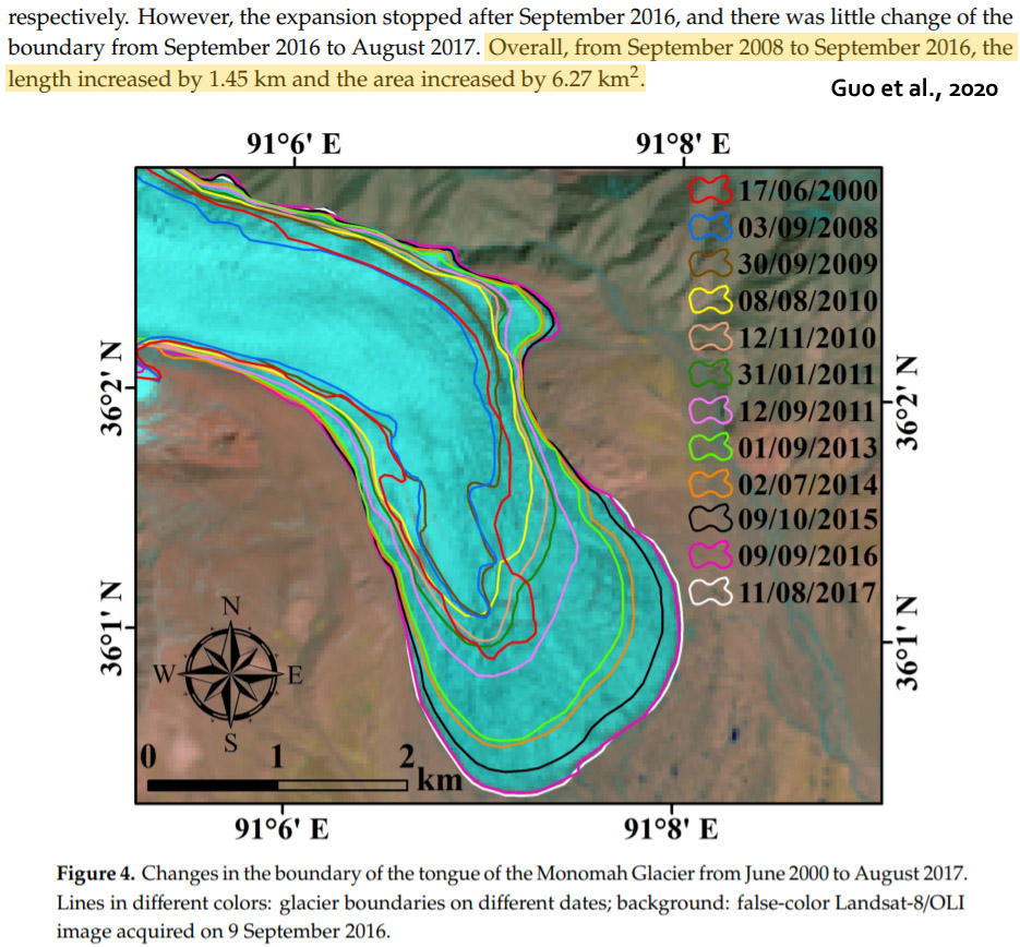
The January 2018 to September 2019 surge of Shisper Glacier, Pakistan, detected from remote sensing observations … The glacier surface velocity profiles indicate that the ablation zone of the glacier continues to be in an active surge phase resulting in advance of the snout and expansion of the ice-dammed lake. Surface glacier velocities are as high as 48 m d−1. Between 18 December 2018 and 8 May 2019, the glacier snout advanced at ~6 m d−1 with a total overall advance of 860 m. The lake formed due to damming of an outflow stream from Mochowar Glacier expanded to its maximum area (29.69 ha) in May 2019 before drainage started on 23 June 2019.
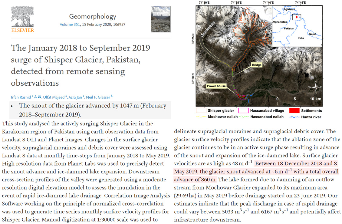
These results provide evidence that marked climate changes may not require an external trigger. The sea-temperature proxy decreased by 1.5°C during the 1300s CE, and the lower temperatures were sustained for centuries. The reconstruction described here provides strong empirical evidence in support of the provocative modeling studies (36–38) that suggest that abrupt multidecadal to century-scale cooling events can arise spontaneously. This interpretation, however, does not exclude the possibility that external forcing—volcanic and solar—may have contributed to the onset and/or development of LIA conditions, as suggested from forced modeling studies (7–11).
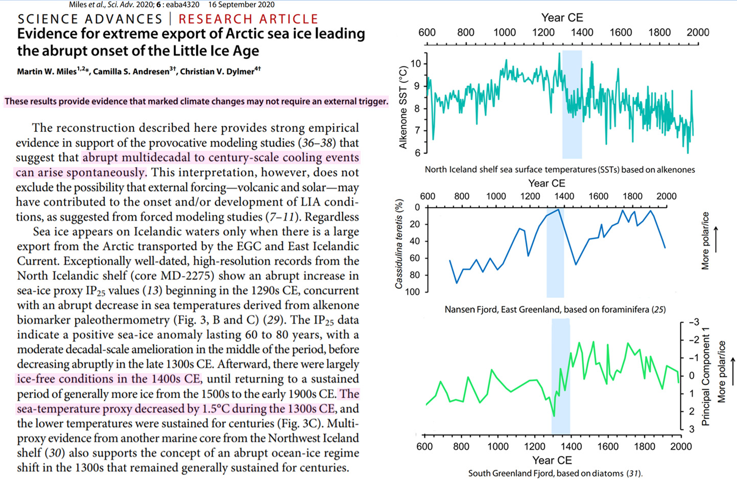
A major driver of the exceptional melting season in 2019 was the persistency of high-pressure systems over the GrIS that promoted an increase in the absorbed solar radiation as well as the flow of warm, moist air along the western portion of the ice sheet towards the north of the ice sheet. The anticyclonic conditions were also responsible for reduced cloudiness in the south and consequent below-average summer snowfall and albedo in this area. In the southwest, dry and sunny conditions dominated. This promoted positive anomalies of the incoming shortwave radiation (Fig. 5g) which, in turn, when combined with the relatively low albedo (due to reduced summer snowfall) promoted positive anomalies of the absorbed shortwave radiation (Fig. 5h) higher than 30 W m−2 … [A]s a result of a quasi permanence of exposure of low-albedo zones, the anomaly of absorbed shortwave radiation was the highest since 1948, with an anomaly integrated over the whole ice sheet of 7.9 W m−2 , 4 times the 1981–2010 standard deviation (inter-annual variability) of 1.9 W m−2 … The exceptional nature of the mass balance components in 2019 was strongly driven by albedo reduction associated with reduced summer snowfall, enhanced absorption of solar radiation, and the flow of warm, moist air along the western portion of the ice sheet.
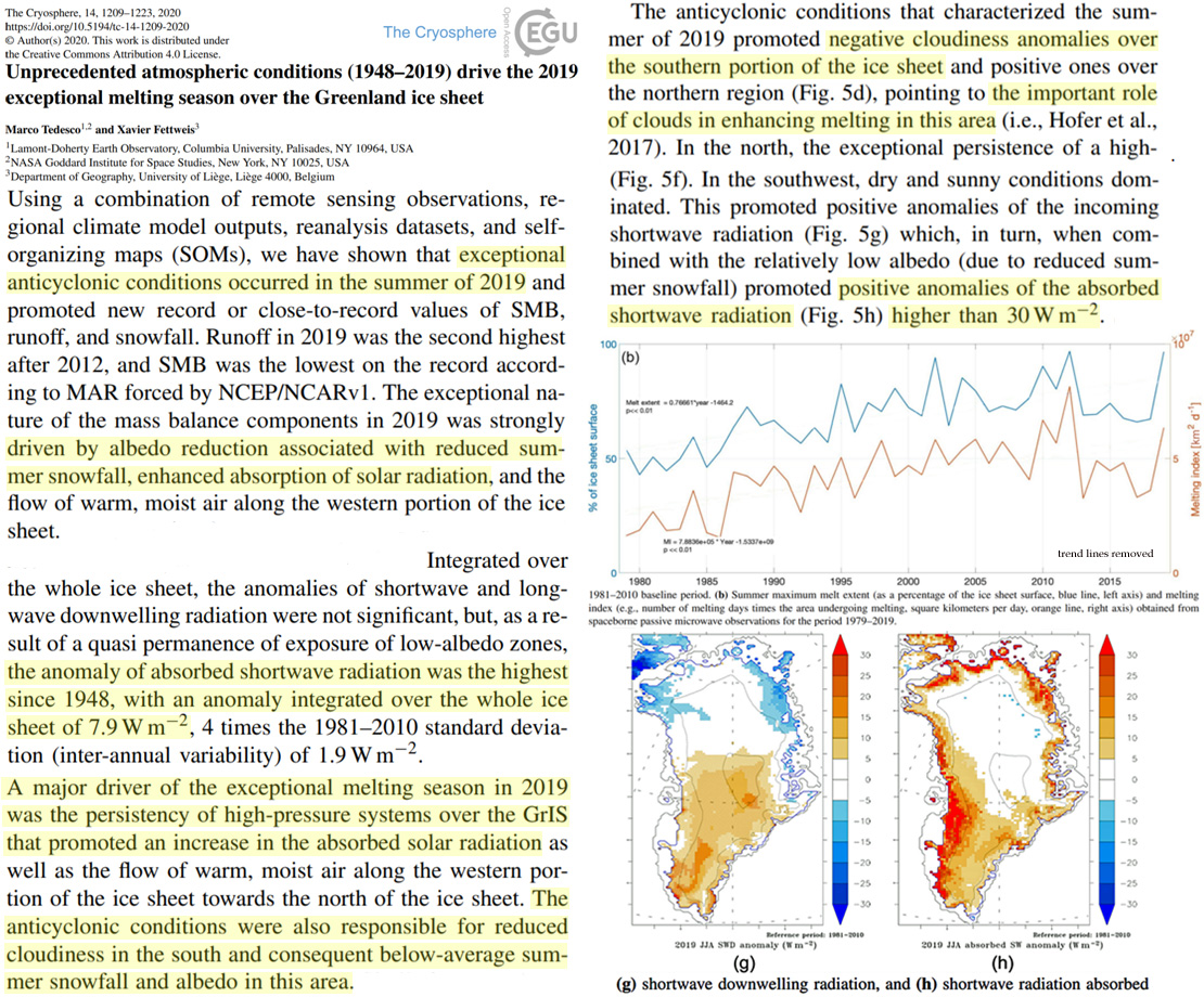
Clouds regulate the amount of radiation received by the surface, which determines surface melt, and can trigger feedback mechanisms that induce albedo changes (Bintanja & Van Den Broeke, 1996). This is the cloud radiative effect (CRE). Clouds block shortwave (SW) radiation which limits the albedo melt feedback, reducing melt. Moreover, clouds directly increase the broadband surface albedo by shifting direct solar radiation to diffuse radiation (Gardner & Sharp, 2010). Yet clouds enhance the amount of longwave (LW) radiation by reemitting the heat lost from the surface, enhancing melt.
Apart from evaluation purposes, in situ SEB data themselves also lead to discovery. For instance, AWS data revealed that occasional melt on the highest parts of the GrIS is especially sensitive to the optical thickness, emissivity, and phase (ice, water, or mixed) of clouds [3, 107] mainly enhancing incoming longwave radiation. In contrast, melt variability in the low-albedo ablation zones is mainly driven by incoming solar radiation (Box and others, 2012), highlighting the complex role of cloud changes on GrIS SMB. Recent results indicate that a decrease in summer cloud cover driven by the above-mentioned increased blocking has largely driven increased SMB losses over the last two decades.
[T]he Holocene sea-level highstand in the Laptev Sea was only reached near 5 cal. ka BP, and sea level was continuing to rise by 7.9 mm yr at c. 6.5 cal. ka BP (Bauch et al. 2001; Klemann et al. 2015). … [D]uring the LGM [Last Glacial Maximum] the Severnaya Zemlya Archipelago was not covered by the Barents-Kara Ice Sheet and that only local ice caps had developed, with sizes comparable to or slightly larger than those of today (Bolshiyanov &Makeyev 1995; Raab et al. 2003; Moller € et al. 2006, 2015). … The peat deposits were 14C-dated to c. 9.8 and 8.6 14C ka BP (11.2 and 9.6 cal. ka BP; Andreevet al. 2008). The pollen spectra in these deposits are characterized by the predominance of Poaceae and Cyperaceae pollen, with high amounts of shrub birch and willow pollen. This supports the suggestion of Bolshiyanov & Makeyev (1995) that the warmest and most humid environmental conditions occurred on the archipelago during the Early Holocene.
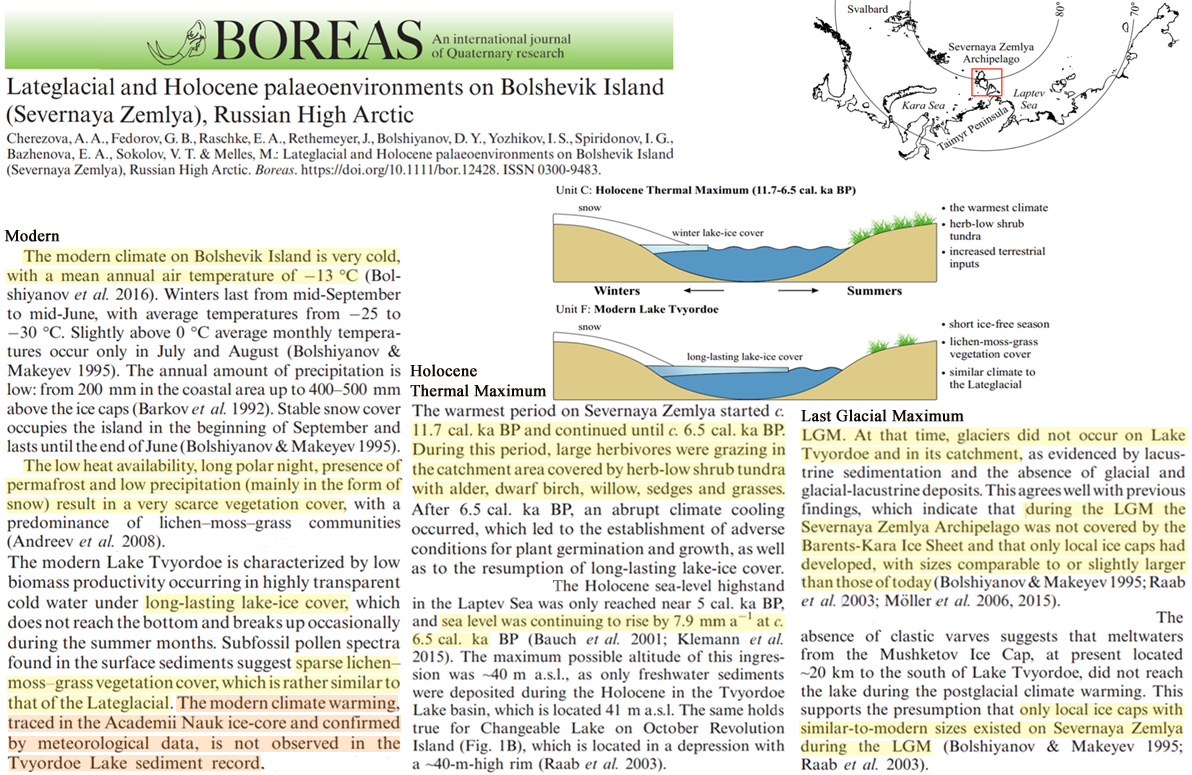
Stable water isotopes and accumulation rates in the Union Glacier region, Ellsworth Mountains, West Antarctica, over the last 35 years … Antarctica is well known to be highly susceptible to atmospheric and oceanic warming. However, due to the lack of long-term and in situ meteorological observations, little is known about the magnitude of the warming and the meteorological conditions in the intersection region between the Antarctic Peninsula (AP), the West Antarctic Ice Sheet (WAIS) and the East Antarctic Ice Sheet (EAIS). Here we present new stable water isotope data (δ18O, δD, d excess) and accumulation rates from firn cores in the Union Glacier (UG) region, located in the Ellsworth Mountains at the northern edge of the WAIS. The firn core stable oxygen isotopes and the d excess exhibit no statistically significant trend for the period 1980–2014, suggesting that regional changes in near-surface air temperature and moisture source variability have been small during the last 35 years.
Arctic sea ice is an important component of the Earth’s climate system, but prior to its recent reduction, its long-term natural instabilities need to be better documented. In this study, information on past sea-ice conditions across the Arctic Ocean demonstrates that whereas its western and central parts remained occupied by perennial sea ice throughout the present interglacial, its southeastern sector close to the Russian margin experienced, at least, sporadic seasonal sea-ice-free conditions during the warmer part of the present interglacial until ∼4,000 y ago. Sea-ice-free conditions during summer in the southeastern Arctic Ocean seem, therefore, to be a recurrent feature linked to its natural variability during warm episodes of the past. … Our new data show positive evidence for some sea-ice opening in the southeastern part of the central Arctic Ocean, during the early and middle Holocene, at least, sporadically. … Whereas these data illustrate a regional behavior of the Arctic sea ice on a decadal to the millennial timescale, they also lead to discard any scenario of its uniform response to climate and paleogeographic variations in the recent geological past.
Our data suggest that during the Early Pleistocene [1.9 million years ago, during a glacial, or ice age], northwestern Greenland was similar to today with substantial ice cover, glacial erosion below warm‐based ice, and coastal ice‐free areas that harbored vegetation. These data suggest the presence of a largely persistent, yet dynamic, ice sheet in northwestern Greenland by the Early Pleistocene (Knutz et al., 2019).
Ice Sheet Melting In High Geothermal Heat Flux Areas
In the present work, the focus is on exploring thermal consequences of melting in isolated localities and its application for determining heat flux beneath ice sheets in Antarctic. A number of parameters control basal ice-sheet temperatures. These include ice thickness, surface temperature, ice accumulation rate and heat transported by horizontal advection. The basal heat gradient is related to the geothermal heat flux, heat produced from basal sliding and heat derived from internal ice deformation.
Greenland is a stable land mass that has preserved ~4 Gyr of Earth’s history. In its vicinity, there are the Mid‐Atlantic Ridge, the Iceland and Jan Mayen hotspots, and a geothermal area in Svalbard, which indicate the complexity of this region. … Rogozhina et al. (2016) suggested that in central and northern Greenland, high GHF [geothermal heat flux] and the weight of the GrIS may cause widespread pressure melting at the bottom of the ice sheet. This idea is reinforced by direct observations of the boundary conditions beneath the GrIS from ice core drilling (Dahl-Jensen et al., 2003a) and the analysis of temporal changes in surface-wave group velocity (Toyokuni et al., 2018). … The distribution of hot springs along the eastern coast of Greenland corresponds to the area where large low-Vp amplitudes are observed. Further, the low-Vp region and the area of high GHF (Figure 8b) are spatially coincident. … The absence of the low-Vp and high GHF region beneath the western basal outcrops is supported by the maximum water temperature of hot springs. The temperature is ~60°C on the east coast, while it is ~20°C on the west coast (Hjartarson and Armannsson, 2010) (Figure 8), suggesting a possible difference in magmatism between the east and west coasts.
Our high-resolution results show that the so-called Iceland plume could be composed of two plumes. One is located directly beneath Iceland but rising from ~1500 km depth, which we call the Iceland plume. The other is rising from the core-mantle boundary beneath central Greenland, which we call the Greenland plume. The Greenland plume has the mainstream and two branches in the lower mantle, and the mainstream rises to the mantle transition zone beneath eastern Greenland. Although the Iceland plume itself is a powerful plume, it may also have three joints with other plumes: the mainstream and a branch of the Greenland plume, and a plume beneath Western Europe, resulting in many active volcanoes in Iceland. The mainstream of the Greenland plume may also supply magmas to the Jan Mayen hotspot and a geothermal area in western Svalbard.
Press release https://polarjournal.ch/en/2020/12/09/greenlands-underground-boosts-thermal-activity-in-the-arctic/
[T]he central part of the Greenland lies above this plume and they suspect that the warmth of the plume influences melting of the Greenland ice sheet.
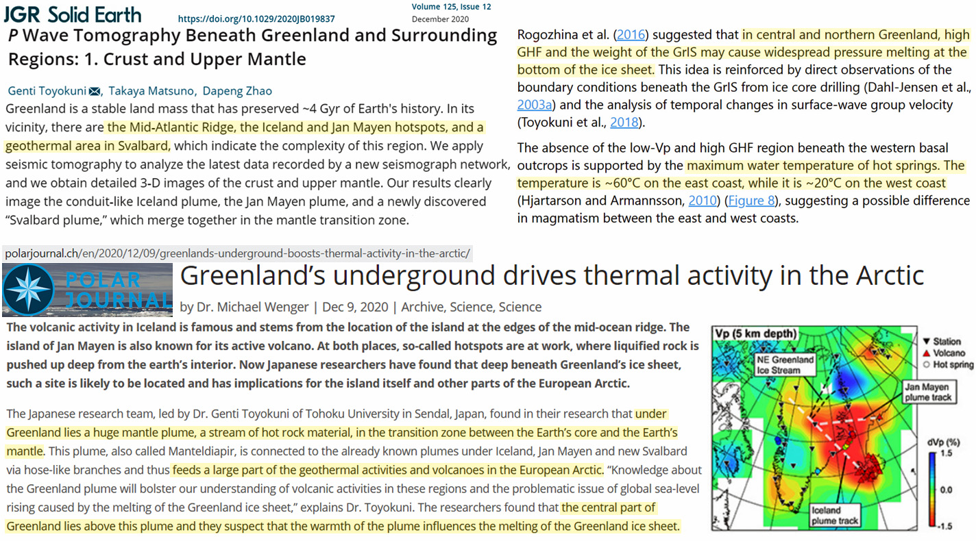
Geothermal heat flux (GHF) impacts the basal thermal regime of ice sheets (Rogozhina and others, 2012; Seroussi and others, 2017). Whether the bed reaches the pressure melting point or not determines whether surface velocities are controlled by sliding at the base or internal deformation. GHF has two main effects on ice dynamics: it affects internal flow through its impact on ice temperature altering the ice rheology (Glen, 1955) and it can increase the sliding rates by providing basal meltwater in regions otherwise not subject to surface water input. Basal meltwater lubricates the bed and thus facilitates sliding. For this reason, high GHF anomalies are thought to initiate and sustain some ice streams (Blankenship and others, 1993; Bourgeois and others, 2000; Fahnestock and others, 2001; Näslund and others, 2005; Bell, 2008; Winsborrow and others, 2010; Rogozhina and others, 2016). … Most studies agree that GHF plays an important role in determining the temperature at the bed, and hence where the bed reaches pressure melting point and how much ice melts in these regions (Greve and Hutter, 1995; Brinkerhoff and others, 2011; Seroussi and others, 2017). Rogozhina and others (2012) did a thorough analysis of the differences between existing GHF maps for the Greenland Ice Sheet and assessed their implication for the thermal regime as well as the ice geometry. They concluded that for paleoclimatic simulations (last 150 ka) the GHF has a major impact on ice topography, in agreement with Greve and Hutter (1995).
Abrupt, Degrees-Per-Decade Natural Global Warming
The Late Antique Little Ice Age, spanning the period from 536CE to roughly 560CE, saw temperatures in the Northern Hemisphere drop by a degree C in less than a decade. This rapid cooling is thought to have caused widespread famine, epidemic disease, and social disruption.
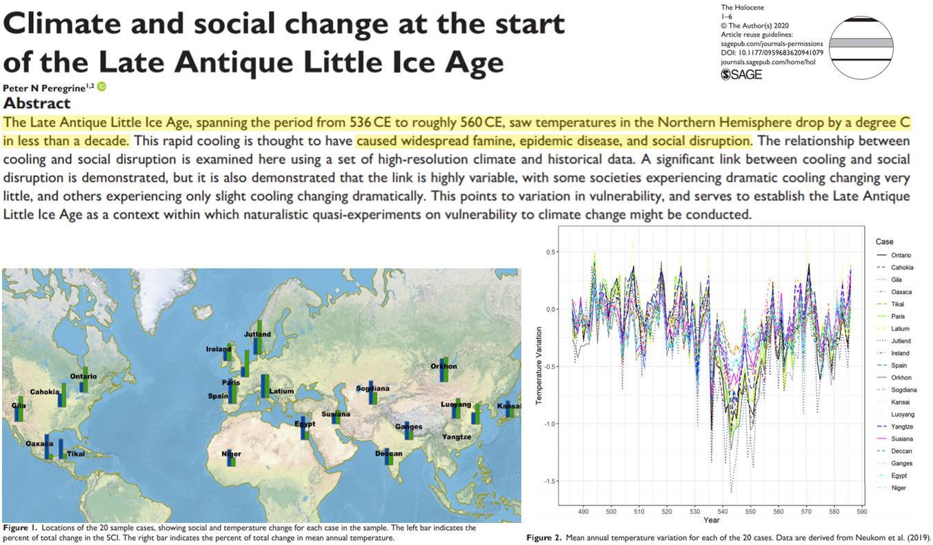


Recent Comments