A Warmer Past: Non-Hockey Stick Reconstructions
Holocene air temperatures were reconstructed from δ18O measurements from the nearby Agassiz Ice Cap. The 25-yr mean annual air temperature record shows a rapid Early Holocene warming, with temperatures being 6–8°C warmer than today at 10,000 yr b2k followed by a gradual cooling to AD 1700 (Lecavalier et al., 2017).
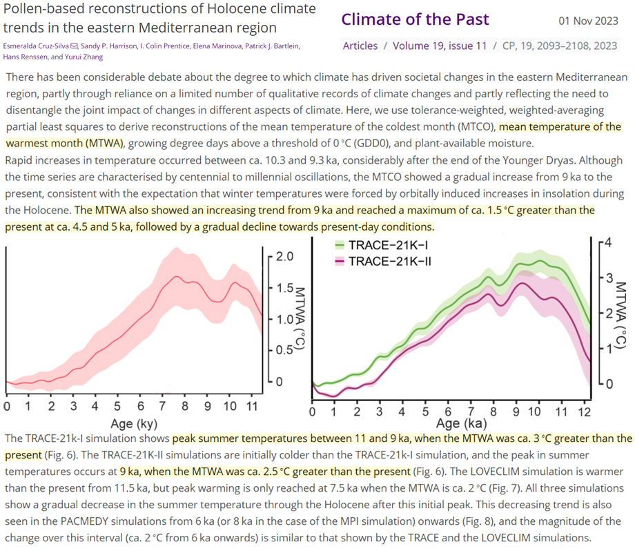
Rapid increases in temperature occurred between ca. 10.3 and 9.3 ka, considerably after the end of the Younger Dryas. Although the time series are characterised by centennial to millennial oscillations, the MTCO showed a gradual increase from 9 ka to the present, consistent with the expectation that winter temperatures were forced by orbitally induced increases in insolation during the Holocene. The MTWA also showed an increasing trend from 9 ka and reached a maximum of ca. 1.5 ∘C greater than the present at ca. 4.5 and 5 ka, followed by a gradual decline towards present-day conditions. … The TRACE-21k-I simulation shows peak summer temperatures between 11 and 9 ka, when the MTWA was ca. 3 ∘C greater than the present
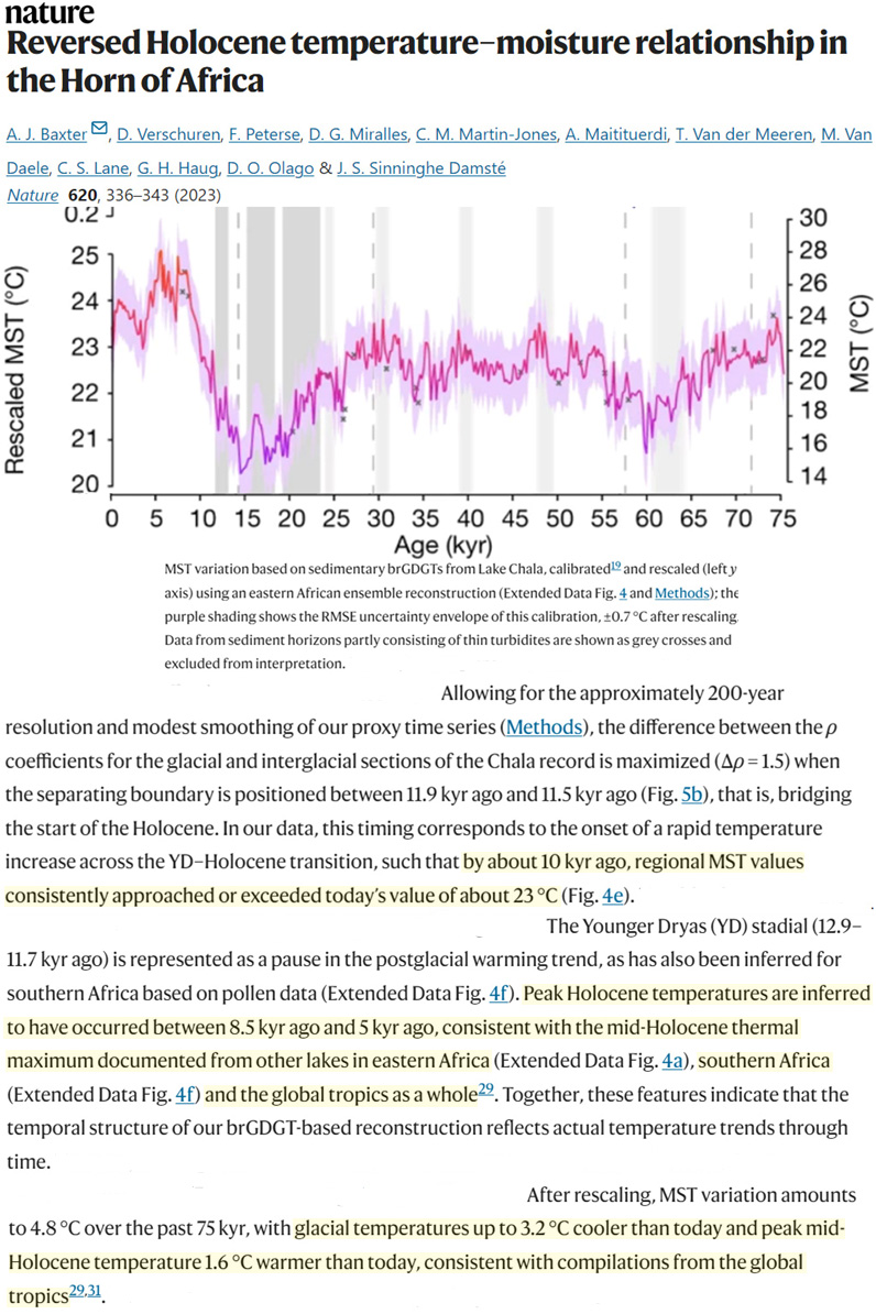
Peak Holocene temperatures are inferred to have occurred between 8.5 kyr ago and 5 kyr ago, consistent with the mid-Holocene thermal maximum documented from other lakes in eastern Africa, southern Africa and the global tropics as a whole. As the focus of this study is on the timing and relative magnitude of past temperature anomalies, we rescaled our brGDGT-based temperature estimates to a regional ensemble reconstruction covering the past 25 kyr based on 7 other currently available temperature records from eastern Africa. After rescaling, MST variation amounts to 4.8 °C over the past 75 kyr, with glacial temperatures up to 3.2 °C cooler than today and peak mid-Holocene temperature 1.6 °C warmer than today, consistent with compilations from the global tropics.
[M]id-Holocene East African temperatures were warmer than today between 8 and 5 ka
Britain and Ireland: glacial landforms during the Bølling–Allerød Interstadial … Climatic reconstructions suggest that peak summer temperatures were warmer than today although the climate was more continental with a greater annual range between winter and summer, accompanied by drier conditions than today. Overall, the interstadial was characterised by negative glacier mass balance and significant reductions in glacier extents across Britain and Ireland. However, it is unknown whether glaciers disappeared entirely. In eastern Scotland, there is evidence that marine ice retreat occurred as late as 13.5 ka, although dating evidence is limited.
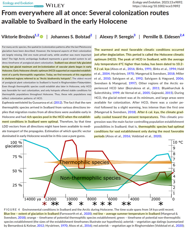
The warmest and most favorable climatic conditions occurred just after deglaciation. This period is called the Holocene climatic optimum (HCO). The peak of HCO in Svalbard, with the average July temperature 6°C higher than today, has been dated to 10.2– 9.2 cal. kya (Alsos et al., 2016; Birks, 1991; Birks et al., 1994; Hald et al., 2004; Hyvärinen, 1970; Mangerud & Svendsen, 2018; Miller et al., 2010; Salvigsen et al., 1992; Salvigsen & Høgvard, 2006; Svendsen & Mangerud, 1997). Other regions of the Arctic experienced HCO later (Bezrukova et al., 2011; Blyakharchuk & Sulerzhitsky, 1999; de Vernal et al., 2005; Gajewski, 2015). During HCO, the glacial extent was at its minimum, and large areas were available for colonization. After HCO, there was a cooler period followed by a slight warming, less intense than the first one (Mangerud & Svendsen, 2018). After 6 cal. kya, the climate gradually cooled toward the present temperatures. This climatic progression was the main factor controlling population establishment possibilities in Svalbard; that is, thermophilic species had optimal conditions for vast establishment only during the most favorable periods (Alsos et al., 2016; Voldstad et al., 2020).
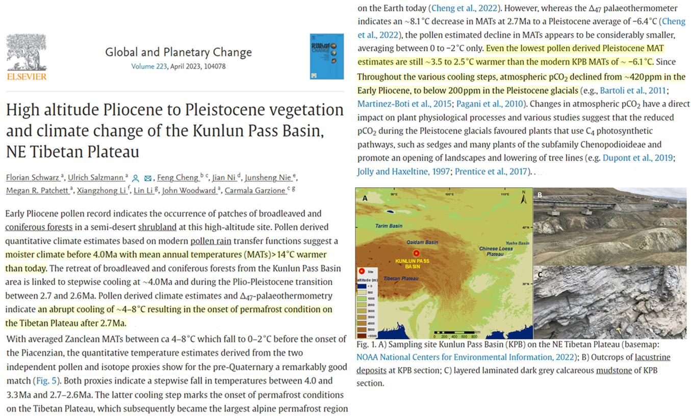
The Early Pliocene pollen record indicates the occurrence of patches of broadleaved and coniferous forests in a semi-desert shrubland at this high-altitude site. Pollen derived quantitative climate estimates based on modern pollen rain transfer functions suggest a moister climate before 4.0 Ma with mean annual temperatures (MATs) > 14 °C warmer than today. … Even the lowest pollen derived Pleistocene MAT estimates are still ∼3.5 to 2.5 °C warmer than the modern KPB MATs of ∼ −6.1 °C.
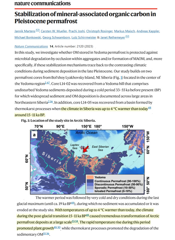
…core L14-05 was recovered from a basin formed by thermokarst processes when the climate in Siberia was up to 4 °C warmer than today around 15–11 ka BP.
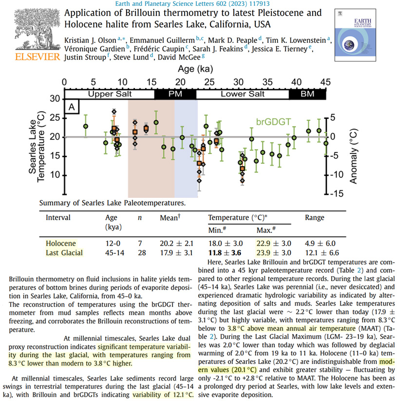
…significant temperature variability during the last glacial, with temperatures ranging from 8.3°C lower than modern to 3.8 °C higher.
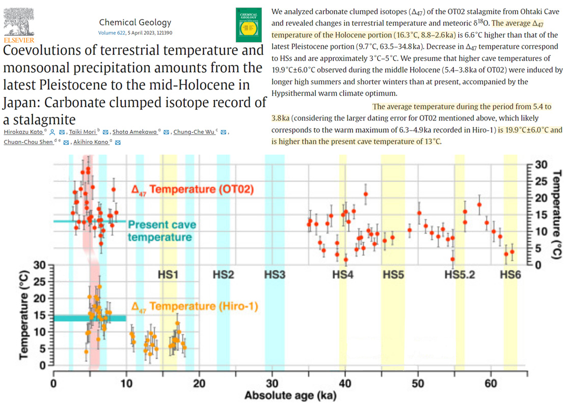
The average temperature during the period from 5.4 to 3.8 ka … is 19.9 °C ± 6.0 °C and is higher than the present cave temperature of 13 °C.
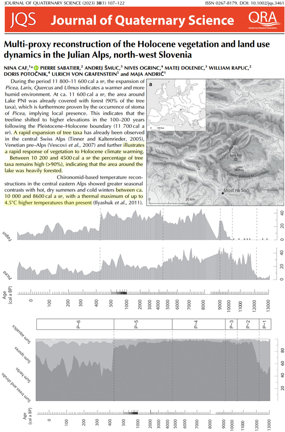
Chironomid‐based temperature reconstructions in the central eastern Alps showed greater seasonal contrasts with hot, dry summers and cold winters between ca. 10 000 and 8600 cal a BP, with a thermal maximum of up to 4.5°C higher temperatures than present (Ilyashuk et al., 2011).
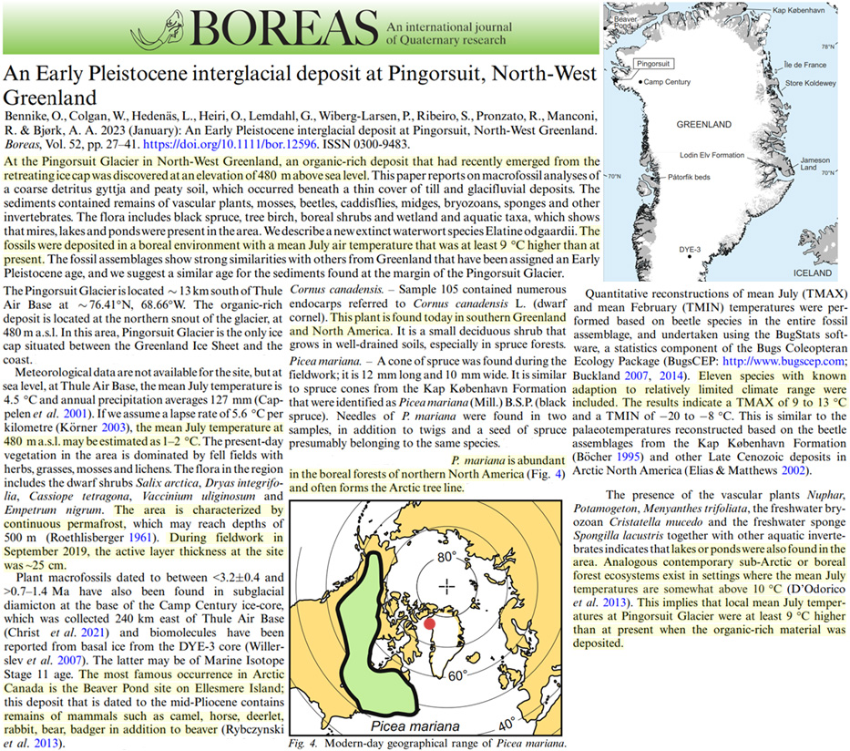
At the Pingorsuit Glacier in North-West Greenland, an organic-rich deposit was discovered at an elevation of 480 m above sea level. The sediments contained remains of vascular plants, mosses, beetles, caddisflies, midges, bryozoans, sponges and other invertebrates. The fossils were deposited in a boreal environment with a mean July air temperature that was at least 9 °C higher than at present.
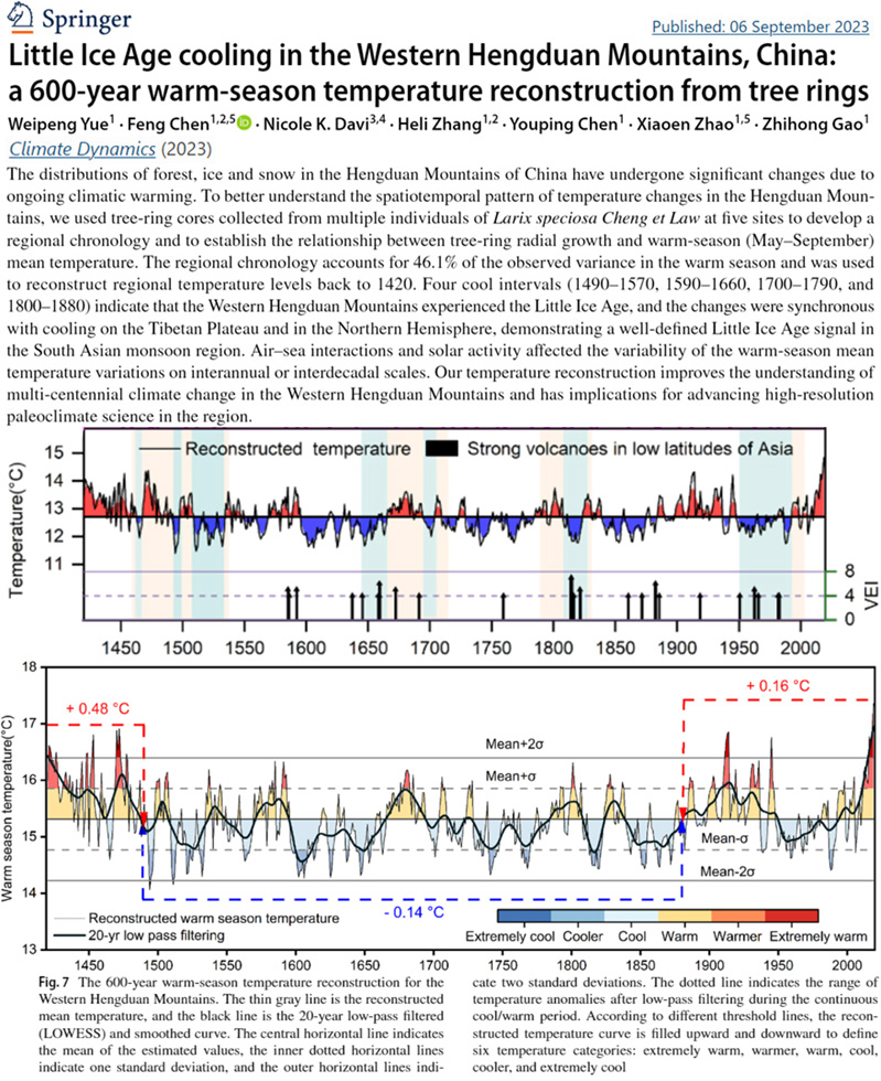
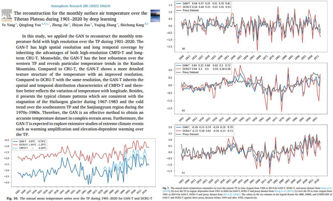
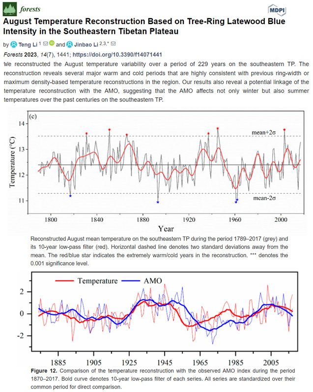
[W]e reconstructed the August temperature variability over a period of 229 years on the southeastern TP. The reconstruction reveals several major warm and cold periods that are highly consistent with previous ring-width or maximum density-based temperature reconstructions in the region. Our results also reveal a potential linkage of the temperature reconstruction with the AMO, suggesting that the AMO affects not only winter but also summer temperatures over the past centuries on the southeastern TP.
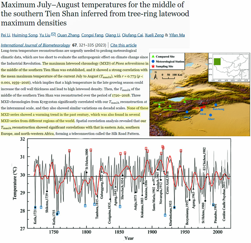
The maximum latewood chronology (MXD)…showed a strong correlation with the mean maximum temperature of the current July to August, with r = 0.77 (p < 0.001, 1959-2016). None of these MXD series [1720-2018] showed a warming trend in the past century, which was also found in several MXD series from different regions of the world.
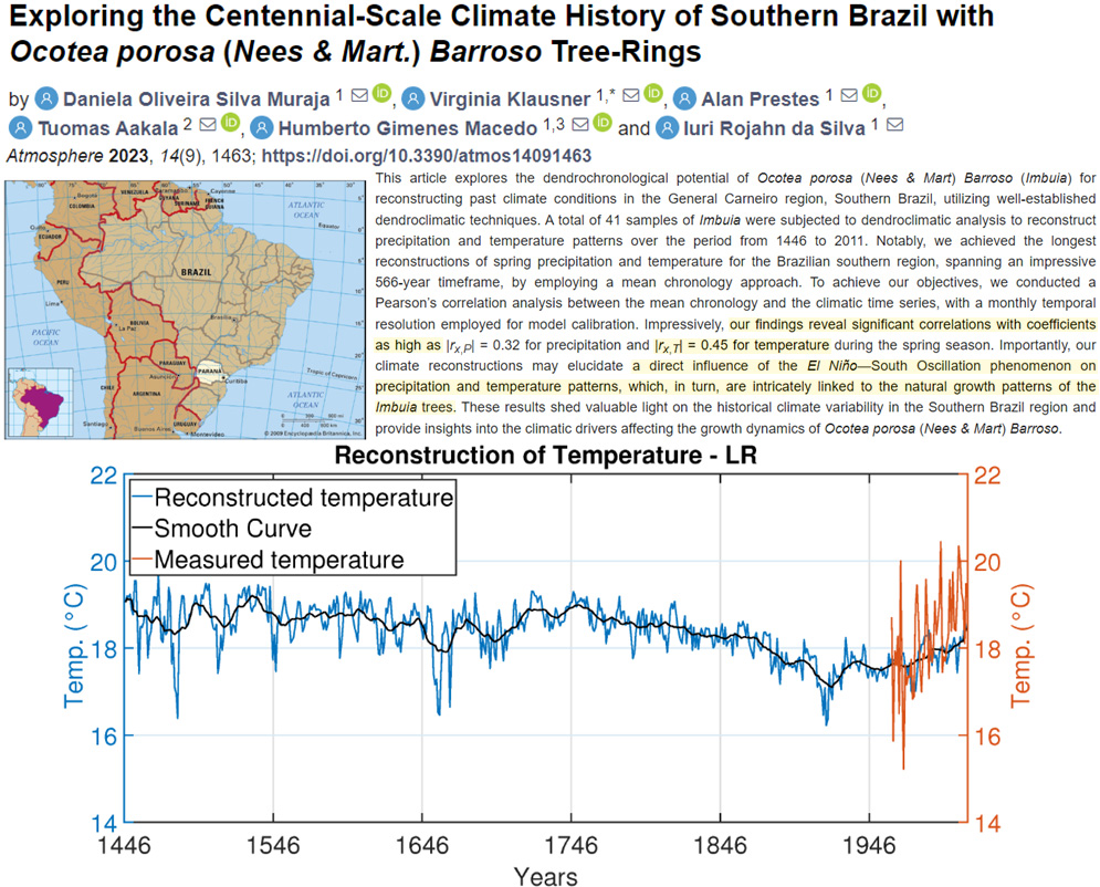
Oliveira Silva Muraja et al., 2023
Non- Global-Scale Warming In Modern Times
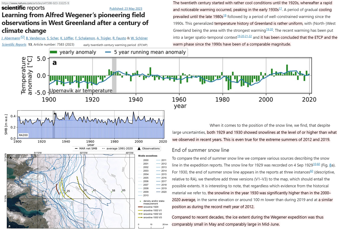
[I]t has been concluded that the early 20th century warming period and the warm phase since the 1990s have been of a comparable magnitude. … [B]oth 1929 and 1930 showed snowlines at the level or higher than what we observed in recent years. This is even true for the extreme summers of 2012 and 2019. … [T]he snowline in the year 1930 was significantly higher than the 2000-2020 average…a similar position as during the record melt year of 2012.
Greenland experienced multiple extreme weather/climate events in recent decades that led to significant melting of the ice sheet. However, how the intensity of extreme climate events over Greenland varied under recent warming has not been fully examined. Here, we collect 176 in situ observations over Greenland and demonstrate that the observed extreme temperature/precipitation events over Greenland are well captured by the RACMO2.3p2 model, in terms of climatological distribution, interannual variability, and long-term trend. Thus, we then investigate the spatiotemporal features of extreme events over Greenland during 1958–2019, using the daily model outputs at 5.5-km resolution. The simulated annual maximum temperature exhibits a significant increasing trend (∼0.13°C decade−1) during 1958–2019, whereas there is a weakening trend (−0.24°C decade−1) in annual minimum temperature over Greenland, especially after the 1990s (−1.24°C decade−1). For the interannual variability, changes in temperature extremes between warm and cold temperature years share large similarities with the distributions of long-term trends.
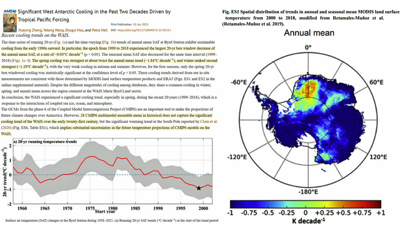
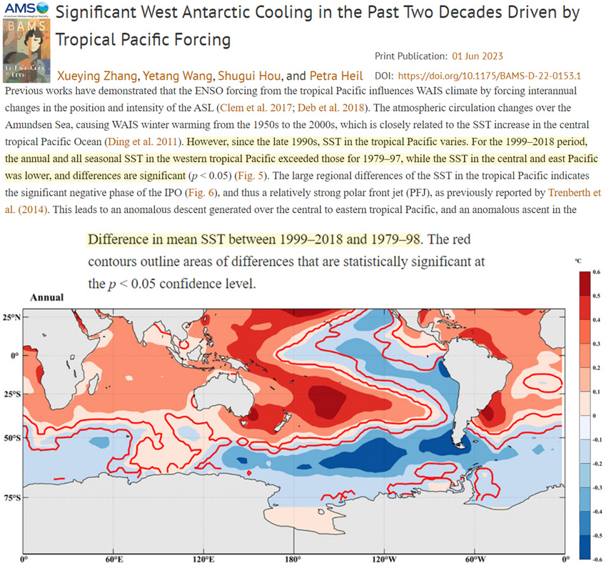
The time series of running 20-yr (Fig. 1a) and the time-varying (Fig. 1b) trends of annual mean SAT at Byrd Station exhibit sustainable cooling from the early 1990s onward. In particular, the epoch from 1999 to 2018 experienced the largest 20-yr box window decrease of the annual mean SAT, at a rate of −0.93°C decade−1 (p < 0.05). The seasonal mean SAT also decreased for the same time interval (1999–2018) (Figs. 1c–f). The spring cooling was strongest at about twice the annual mean trend (−1.84°C decade−1), and winter ranked second strongest (−1.19°C decade−1), with the very weak cooling in autumn and summer. However, for the four seasons, only the spring 20-yr box windowed cooling was statistically significant at the confidence level of p < 0.05. These cooling trends derived from our in situ measurements are consistent with those determined by MODIS land surface temperature products and ERA5 (Figs. ES1 and ES2 in the online supplemental material). Despite the different magnitudes of cooling among databases, they share a common cooling in winter, spring, and annual mean across the region centered at the WAIS Marie Byrd Land sector.
Lack Of Anthropogenic/CO2 Signal In Sea Level Rise
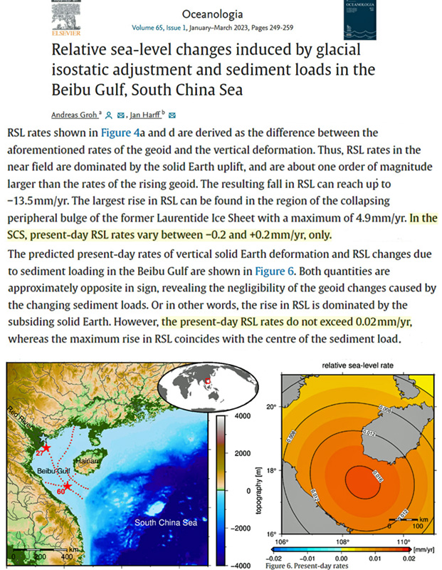
In the SCS, present-day RSL rates vary between -0.2 and +0.2 mm/yr, only. … the present-day RSL rates do not exceed 0.02 mm/yr
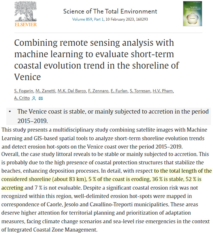
The Venice coast is stable, or mainly subjected to accretion in the period 2015–2019. … This study presents a multidisciplinary study combining satellite images with Machine Learning and GIS-based spatial tools to analyze short-term shoreline evolution trends and detect erosion hot-spots on the Venice coast over the period 2015–2019. … Overall, the case study littoral reveals to be stable or mainly subjected to accretion. This is probably due to the high presence of coastal protection structures that stabilize the beaches, enhancing deposition processes. In detail, with respect to the total length of the considered shoreline (about 83 km), 5 % of the coast is eroding, 36 % is stable, 52 % is accreting and 7 % is not evaluable.
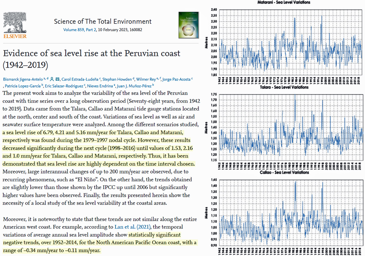
Among the different scenarios studied, a sea level rise of 6.79, 4.21 and 5.16 mm/year for Talara, Callao and Matarani, respectively was found during the 1979–1997 nodal cycle. However, these results decreased significantly during the next cycle (1998–2016) until values of 1.53, 2.16 and 1.0 mm/year for Talara, Callao and Matarani, respectively. Thus, it has been demonstrated that sea level rise are highly dependent on the time interval chosen. … Moreover, it is noteworthy to state that these trends are not similar along the entire American west coast. For example, according to Lan et al. (2021), the temporal variations of average annual sea level amplitude show statistically significant negative trends, over 1952–2014, for the North American Pacific Ocean coast, with a range of −0.34 mm/year to −0.11 mm/year.
Sea Levels Multiple Meters Higher When CO2 <280 ppm
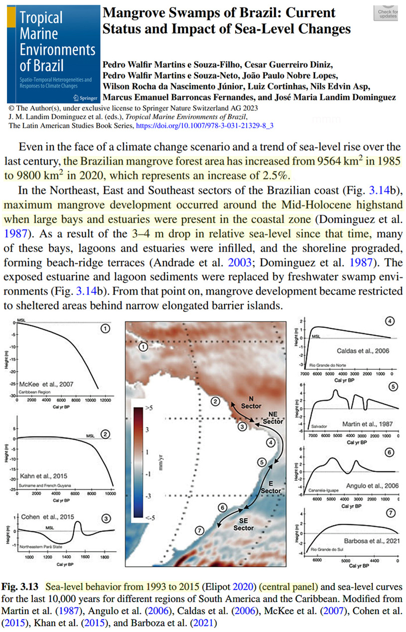
Even in the face of a climate change scenario and a trend of sea-level rise over the last century, the Brazilian mangrove forest area has increased from 9564 km2 in 1985 to 9800 km2 in 2020, which represents an increase of 2.5%. … [I]n the Northeast, East, and Southeast sectors, the sea-level trajectories were completely different, with a highstand at 6000–7000 Cal year. BP followed by a 3- to 4-m sea-level drop.
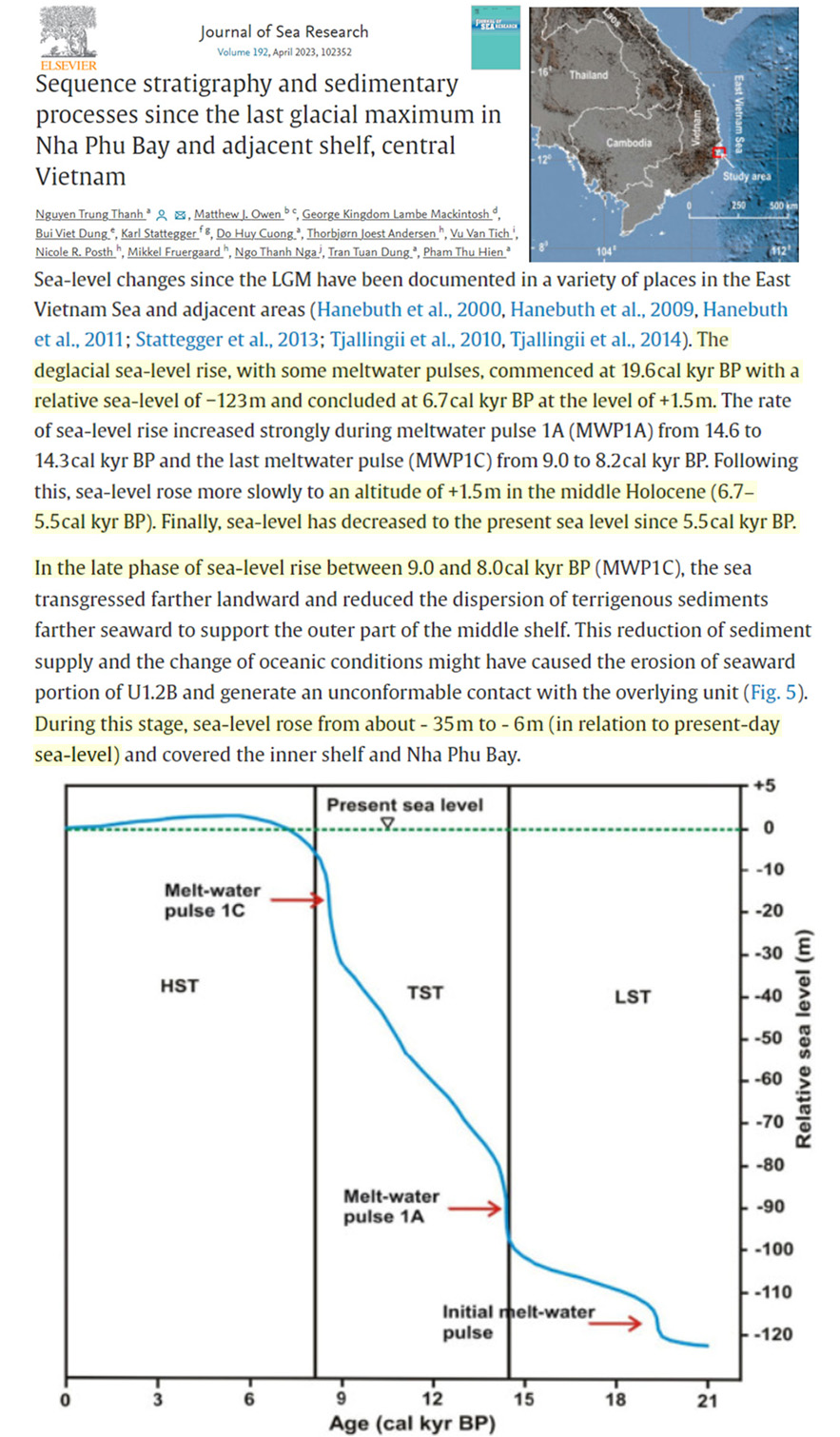
Sea-level changes since the LGM have been documented in a variety of places in the East Vietnam Sea and adjacent areas (Hanebuth et al., 2000, Hanebuth et al., 2009, Hanebuth et al., 2011; Stattegger et al., 2013; Tjallingii et al., 2010, Tjallingii et al., 2014). The deglacial sea-level rise, with some meltwater pulses, commenced at 19.6 cal kyr BP with a relative sea-level of −123 m and concluded at 6.7 cal kyr BP at the level of +1.5 m. The rate of sea-level rise increased strongly during meltwater pulse 1A (MWP1A) from 14.6 to 14.3 cal kyr BP and the last meltwater pulse (MWP1C) from 9.0 to 8.2 cal kyr BP. Following this, sea-level rose more slowly to an altitude of +1.5 m in the middle Holocene (6.7–5.5 cal kyr BP). Finally, sea-level has decreased to the present sea level since 5.5 cal kyr BP.
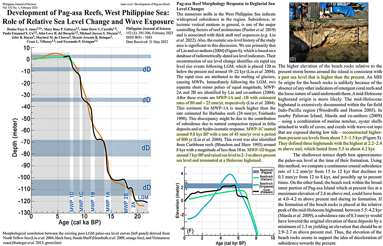
The higher elevation of the beach rocks relative to the present storm berms around the island is consistent with a past sea level that is higher than the present. … Beach rock exposures indicate the occurrence of a relative highstand that is greater than 2 m within the Pagasa area during the mid-Holocene. … On the other hand, the beach rock within the broad inner portion of Pag-asa Island which at present lies at a maximum elevation of 2.6 m above msl, could have been at 4.0–4.2 m above present msl during its formation. If the formation of the beach rocks is placed at the relative peak of the mid-Holocene highstand, between 5.5–4.2 kyr (Maeda et al. 2009), a subsidence rate of 0.3 mm/yr would have lowered the original elevation of these deposits by a minimum of 1.3 m yielding an elevation that should be at 2.9–2.7 m above present msl. … MWP-1C started around 9.8 kyr BP with a rate of 45 mm/yr over a period of 800 yr (Liu et al. 2004). This event was also identified from Caribbean reefs (Blanchon and Shaw 1995) around 8 kyr with a magnitude of less than 10 m. MWP-1D began around 7 kyr BP and raised sea level to 2–3 m above present sea level and terminated at a Holocene highstand. … [E]stimated [sea level rise] rates of 80 and ~25 mm/yr … MWP-1C started around 9.8 kyr BP with a rate of 45 mm/yr over a period of 800 yr
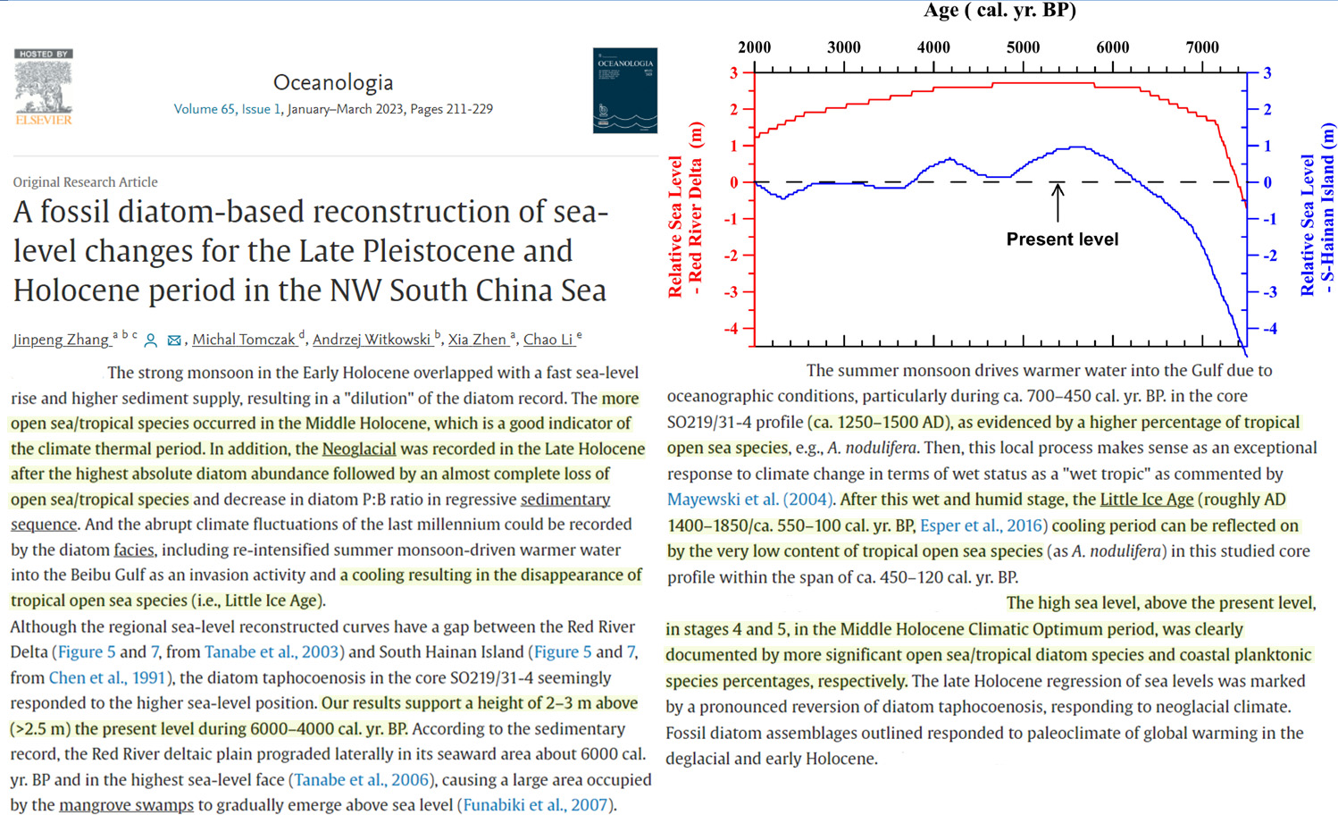
Our results support a height of 2–3 m above (>2.5 m) the present level during 6000–4000 cal. yr. BP. …. The strong monsoon in the Early Holocene overlapped with a fast sea-level rise and higher sediment supply, resulting in a “dilution” of the diatom record. The more open sea/tropical species occurred in the Middle Holocene, which is a good indicator of the climate thermal period. In addition, the Neoglacial was recorded in the Late Holocene after the highest absolute diatom abundance followed by an almost complete loss of open sea/tropical species and decrease in diatom P:B ratio in regressive sedimentary sequence. And the abrupt climate fluctuations of the last millennium could be recorded by the diatom facies, including re-intensified summer monsoon-driven warmer water into the Beibu Gulf as an invasion activity and a cooling resulting in the disappearance of tropical open sea species (i.e., Little Ice Age).
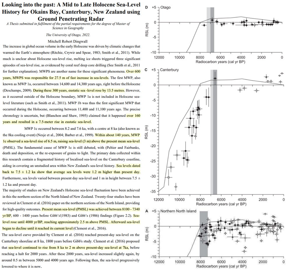
Sea levels dated back to 7.5 ± 1.2 ka show that average sea levels were 1.2 m higher than present day. Furthermore, sea levels varied between present day sea-level and 1 m in height between 7.5 ± 1.2 ka and present day.
During the last 5,000 years, the major accretion-islet episodes occurred irrespective of the course of sea level, indicating that sea-level change was not a driver of islet accretion. Periodical, marine high-energy events clearly appear to be the key controls of islet shaping. Shifts of cyclone source areas further south and increasing cyclone intensity, but lower frequency, due to enhanced enso variability throughout the 21st century, is postulated to expose the Gambier island Group to stronger, but fewer disturbance events when compared to the last millennia. .. After a rapid postglacial rise (Bard et al., 1996), sea level reached and outpassed its present position by approximately 6,000 cal yr. Sea level continued to rise up irregularly to heights of about + 1 m relative to pmsl, from 5,000 to 4,100 cal yr, then remained stable over a period of about 600 years. From about 3,400 yr BP, sea level started to fall progressively (Hallmann et al., 2020). Between 3,000 and 1,500 cal yr, sea level dropped step by step reaching its modern position during the last millennium (Pirazzoli and Montaggioni, 1986, 1987, 1988a, b; Hallmann et al., 2018, 2020). … [I]n the north-west Tuamotu, on Takapoto Atoll, motu would have developed during the sea-level drop phase from 2,500 yr BP to present (Montaggioni et al., 2018, 2019). However, there is no evidence that the position of sea level during its course has played a significant role in atoll-islet building.
…the Middle Holocene, the relative sea level peaked 1–3 m above the present level
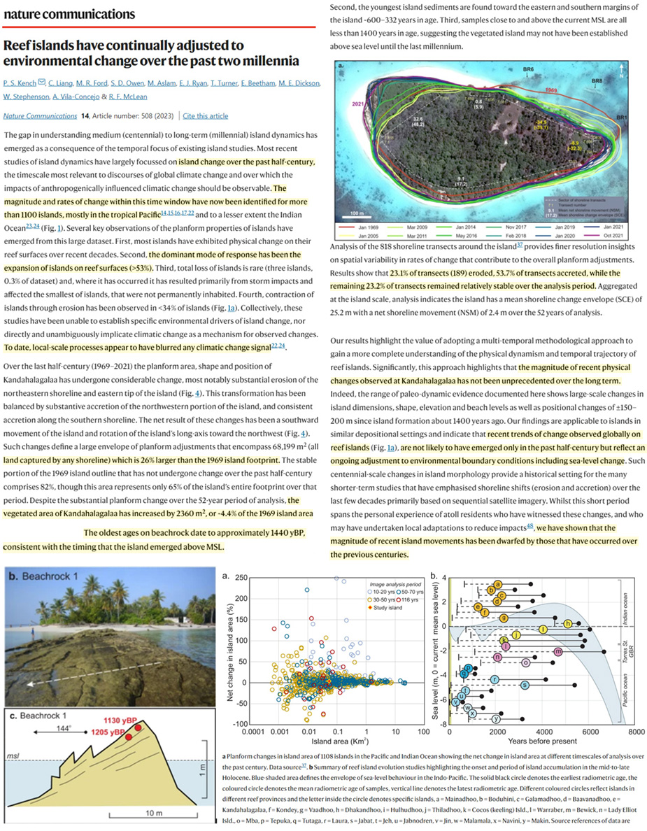
Results show the magnitude of island change over the past half-century (±40 m movement) is not unprecedented compared with paleo-dynamic evidence that reveals large-scale changes in island dimension, shape, beach levels, as well as positional changes of ±200 m since island formation ~1,500 years ago.
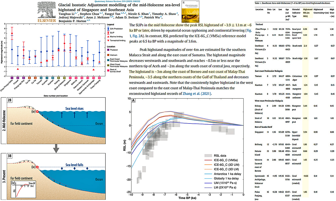
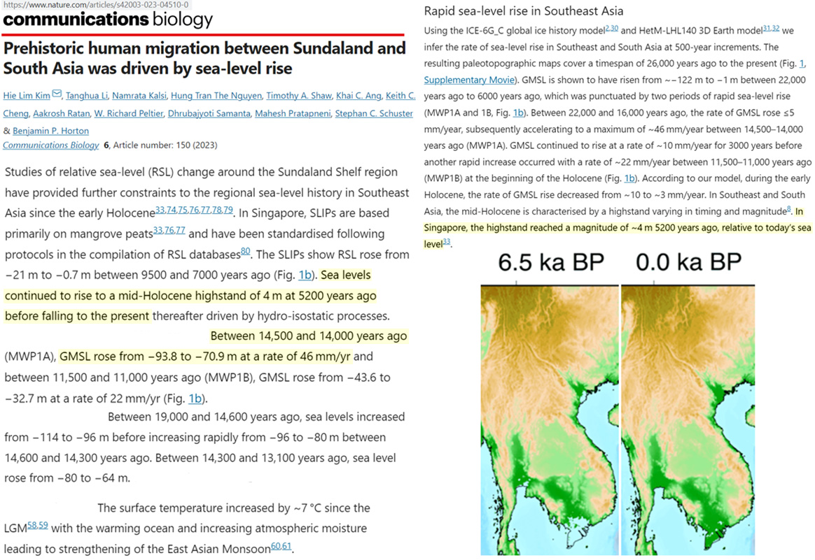
The highstand expanded outwards and reached the highest levels (~4.5 m) in Southeast Asia at 6.5 ka BP and decreased afterwards … The SLIPs in the mid Holocene show the peak RSL highstand of ~3.9 ± 1.1 m at ~6 ka BP.
In this study the Late Holocene development of the Varna Lake is compiled. It demonstrates the pulsating sea-lake connection with a maximum marine influence. The stage is marked by the presence of marine sediments and has a radiocarbon dating at 1720 cal. yr. BP (in the borehole Zv_2). … The identified three facies settings exist simultaneously and prove the oscillatory nature of the emerging Late Holocene transgression – the Nymphaean transgression, which started about 2000 years ago. The stage relates to the Subatlantic according to the Alpine stratigraphical scale, to the Dzemetinian layers (Nevesskaya, 1965) and is correlated with the New Black Sea regional substages (Shopov, 1991). As а result of the transgressive phase, the sea level rose to about 1–1.5 m above the current sea level. The coastal area on the two sides of the Varna Lake, as well as the existing ancient settlements, were gradually submerged.
Gupta and Bhoolokam Rajani, 2023
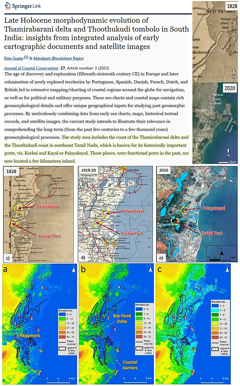
By meticulously combining data from early sea charts, maps, historical textual records, and satellite images, the current study intends to illustrate their relevance in comprehending the long-term (from the past few centuries to a few thousand years) geomorphological processes. The study area includes the coast of the Thamirabarani delta and the Thoothukudi coast in southeast Tamil Nadu, which is known for its historically important ports, viz. Korkai and Kayal or Palayakayal. These places, were functional ports in the past, are now located a few kilometres inland.
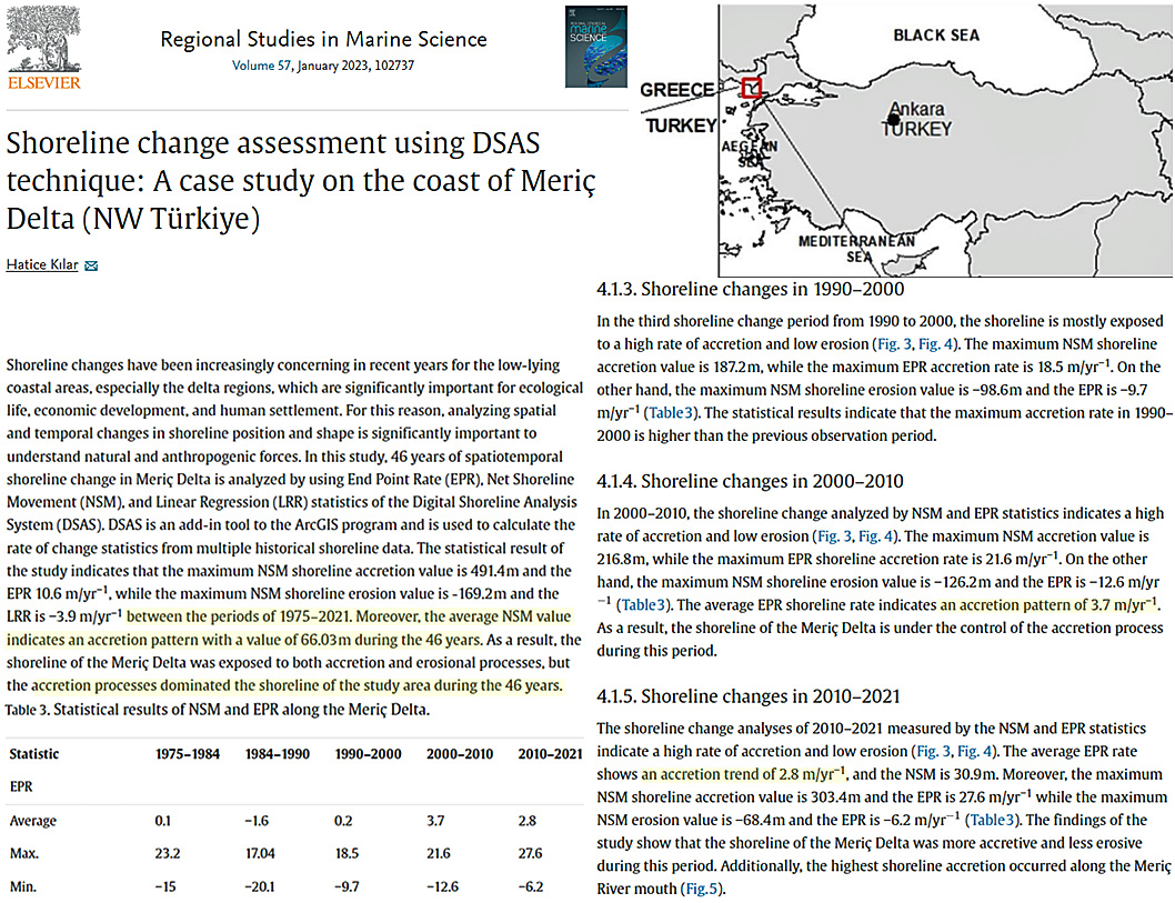
The statistical result of the study indicates that the maximum NSM shoreline accretion value is 491.4 m and the EPR 10.6 m/yr−1, while the maximum NSM shoreline erosion value is -169.2 m and the LRR is −3.9 m/yr−1 between the periods of 1975–2021. Moreover, the average NSM value indicates an accretion pattern with a value of 66.03 m during the 46 years. As a result, the shoreline of the Meriç Delta was exposed to both accretion and erosional processes, but the accretion processes dominated the shoreline of the study area during the 46 years.
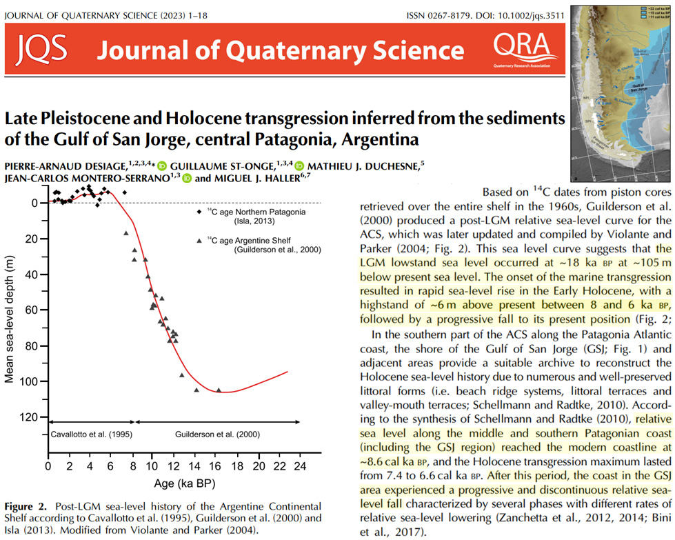
This sea level curve suggests that the LGM lowstand sea level occurred at ~18 ka BP at ~105 m below present sea level. The onset of the marine transgression resulted in rapid sea‐level rise in the Early Holocene, with a highstand of ~6 m above present between 8 and 6 ka BP, followed by a progressive fall to its present position
The eustatic sea level curve shows that sea level reached a Holocene maximum high stand approximately 2.5 m above the present level 6 000 years ago (Fig.7b). Thereafter, sea level fell to the present level without large fluctuations, being approximately ±0.5 m above/ below its present sea level 3 000 years ago (Xu et al., 2018).
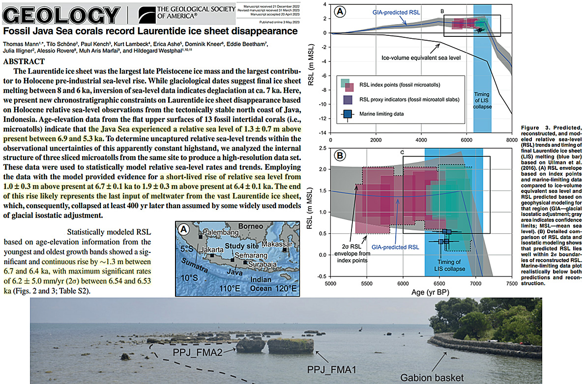
Age-elevation data from the flat upper surfaces of 13 fossil intertidal corals (i.e., microatolls) indicate that the Java Sea experienced a relative sea level of 1.3 ± 0.7 m above present between 6.9 and 5.3 ka. To determine uncaptured relative sea-level trends within the observational uncertainties of this apparently constant highstand, we analyzed the internal structure of three sliced microatolls from the same site to produce a high-resolution data set. These data were used to statistically model relative sea-level rates and trends. Employing the data with the model provided evidence for a short-lived rise of relative sea level from 1.0 ± 0.3 m above present at 6.7 ± 0.1 ka to 1.9 ± 0.3 m above present at 6.4 ± 0.1 ka. The end of this rise likely represents the last input of meltwater from the vast Laurentide ice sheet, which, consequently, collapsed at least 400 yr later than assumed by some widely used models of glacial isostatic adjustment.
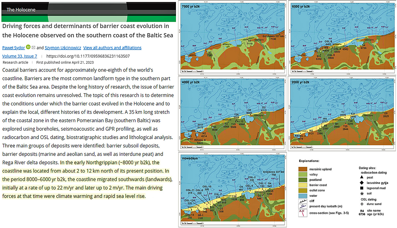
In the period 8000–6000 yr b2k, the coastline migrated southwards (landwards), initially at a rate of up to 22 m/yr and later up to 2 m/yr. The main driving forces at that time were climate warming and rapid sea level rise.
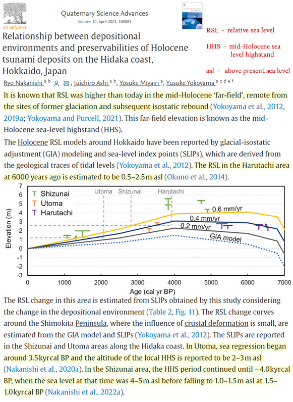
It is known that RSL was higher than today in the mid-Holocene ‘far-field’, remote from the sites of former glaciation and subsequent isostatic rebound (Yokoyama et al., 2012, 2019a; Yokoyama and Purcell, 2021). This far-field elevation is known as the mid-Holocene sea-level highstand (HHS). … The Holocene RSL models around Hokkaido have been reported by glacial-isostatic adjustment (GIA) modeling and sea-level index points (SLIPs), which are derived from the geological traces of tidal levels (Yokoyama et al., 2012). The RSL in the Harutachi area at 6000 years ago is estimated to be 0.5–2.5 m asl [above present sea level] (Okuno et al., 2014). … In Utoma, sea regression began around 3.5 kyr cal BP and the altitude of the local HHS is reported to be 2–3 m asl (Nakanishi et al., 2020a). In the Shizunai area, the HHS period continued until ∼4.0 kyr cal BP, when the sea level at that time was 4–5 m asl before falling to 1.0–1.5 m asl at 1.5–1.0 kyr cal BP (Nakanishi et al., 2022a).
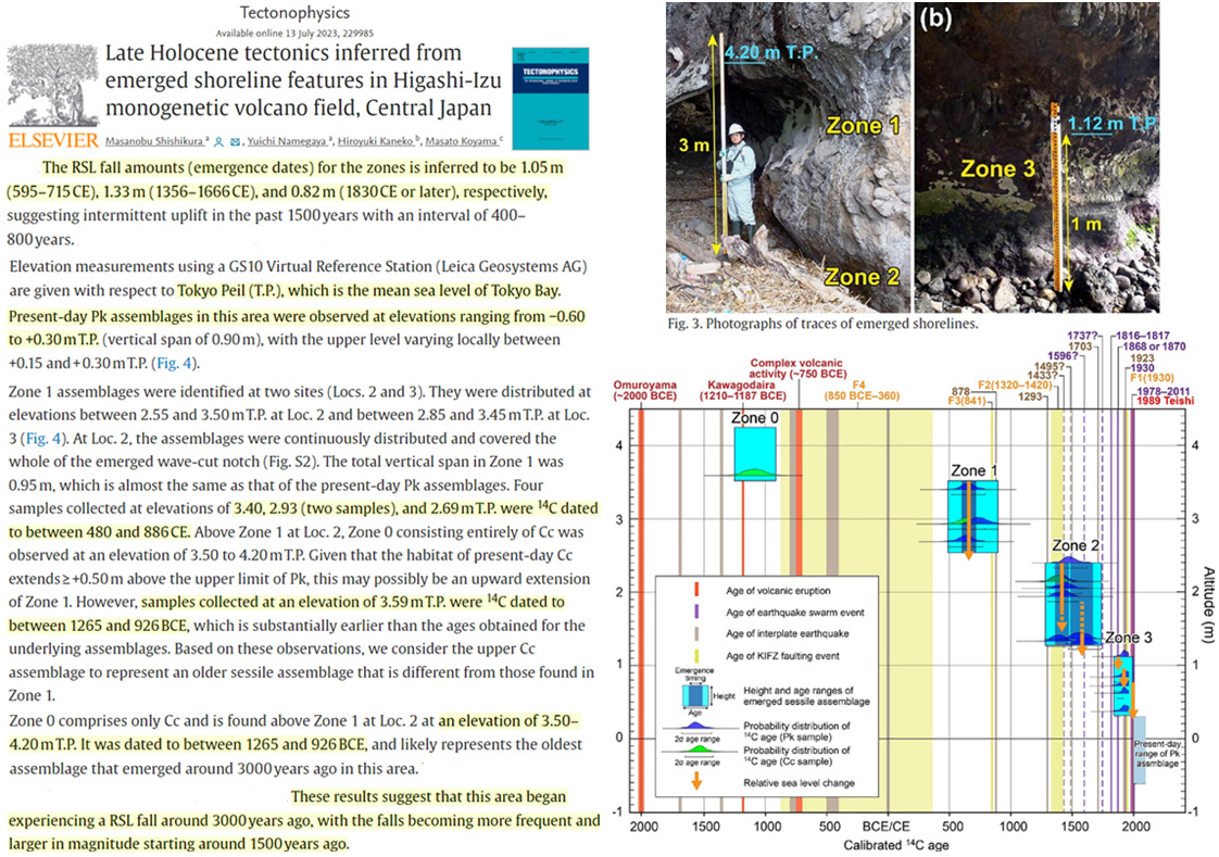
[S]amples collected at an elevation of 3.59 m T.P. [above present Tokyo Peil sea level] were [carbon dated] to between 1265 and 926 BCE. … These results suggest that this area began experiencing a RSL [relative sea level] fall around 3000 years ago, with the falls becoming more frequent and larger in magnitude starting around 1500 years ago.
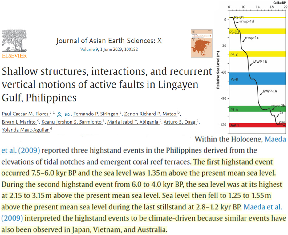
Within the Holocene, Maeda et al. (2009) reported three highstand events in the Philippines derived from the elevations of tidal notches and emergent coral reef terraces. The first highstand event occurred 7.5–6.0 kyr BP and the sea level was 1.35 m above the present mean sea level. During the second highstand event from 6.0 to 4.0 kyr BP, the sea level was at its highest at 2.15 to 3.15 m above the present mean sea level. Sea level then fell to 1.25 to 1.55 m above the present mean sea level during the last stillstand at 2.8–1.2 kyr BP. Maeda et al. (2009) interpreted the highstand events to be climate-driven because similar events have also been observed in Japan, Vietnam, and Australia.
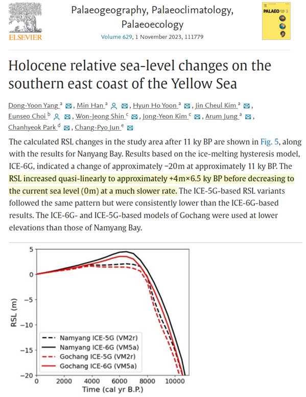
The RSL increased quasi-linearly to approximately +4 m × 6.5 ky BP before decreasing to the current sea level (0 m) at a much slower rate.
Using the ICE-6G_C global ice history model2,30 and HetM-LHL140 3D Earth model31,32 we infer the rate of sea-level rise in Southeast and South Asia at 500-year increments. The resulting paleotopographic maps cover a timespan of 26,000 years ago to the present (Fig. 1, Supplementary Movie). GMSL is shown to have risen from ~−122 m to −1 m between 22,000 years ago to 6000 years ago, which was punctuated by two periods of rapid sea-level rise (MWP1A and 1B, Fig. 1b). Between 22,000 and 16,000 years ago, the rate of GMSL rose ≤5 mm/year, subsequently accelerating to a maximum of ~46 mm/year between 14,500–14,000 years ago (MWP1A). GMSL continued to rise at a rate of ~10 mm/year for 3000 years before another rapid increase occurred with a rate of ~22 mm/year between 11,500–11,000 years ago (MWP1B) at the beginning of the Holocene (Fig. 1b). According to our model, during the early Holocene, the rate of GMSL rise decreased from ~10 to ~3 mm/year. In Southeast and South Asia, the mid-Holocene is characterised by a highstand varying in timing and magnitude. In Singapore, the highstand reached a magnitude of ~4 m 5200 years ago, relative to today’s sea level.
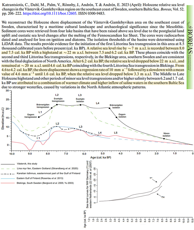
Our results indicate that the initiation of the Littorina Sea transgression (L1) took place at c. 8.5 cal. ka BP followed by a 7-m rise in relative sea level reaching an altitude of 22 m a.s.l. after 7.7 cal. ka BP. A maximum highstand at this altitude is evident from 7.5 to 6.2 cal. ka BP. These phases coincide with the second and third Littorina Sea transgressions, respectively, in the Lina Myr, eastern Gotland and the Blekinge area, southern Sweden. Higher primary productivity mainly between 6.9 and 6.2 cal. ka BP can likely be attributed to more saline and warm conditions associated with the sea level transgression and the Holocene optimum. After 6.2 cal. kaBP, the relative sea level dropped below 22 m a.s.l., although it remained at an altitude of 20 m a.s.l. until 4.6 cal. ka BP.The maximum transgression after 8.0 cal. ka BP and the highstand between 7.5 and 6.2 cal. ka BP are associated with eustatic sea level rise and are consistent with the final phase of North American deglaciation. During the Late Holocene, the highstand until c. 4.6 cal. ka BP and periods of minor transgressions and/or higher salinity are attributed to warmer climate and the high inflow of saline water in the southern Baltic Sea
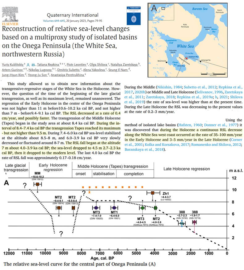
This study allowed us to obtain new information about the transgressive-regressive stages of the White Sea in the Holocene. However, the question of the time of the beginning of the late glacial transgression, as well as its maximum level, remained unanswered. The regression of the Early Holocene in the center of the Onega Peninsula was not higher than 11 m before10.6–10.2 ka cal BP, and not higher than 7 m – before9.4–9.1 ka cal BP. The RSL decreased at a rate of 0.4 cm/year, and possibly faster. The transgression of the Middle Holocene (Tapes) began in the study area at about 8.4 ka cal BP. During the interval of 8.4–7.4 ka cal BP the transgression Tapes reached its maximum – but not higher than 9.5 m. During 7.4–6.0 ka cal BP sea-level stabilized at the altitude about 8.5–8 m, and 6.0–3.9 ka cal BP very slowly decreased or fluctuated around 8-7 m. The RSL fall began at the altitude 7 m about 4.0–3.9 ka cal BP; the sea-level dropped to 4.5 m 2.7–2.3 ka cal BP, then it dropped to the modern level. The last 4.0 ka cal BP the rate of RSL fall was approximately 0.17–0.18 cm/year. Since the Middle Holocene transgression, the relief and sediments of the coast have been affected by fluctuations in the level during storm surges. They also have a destructive effect on indicators of long-term sea-level rise.
Geothermal Heat Flow Melts Ice Sheets From Below
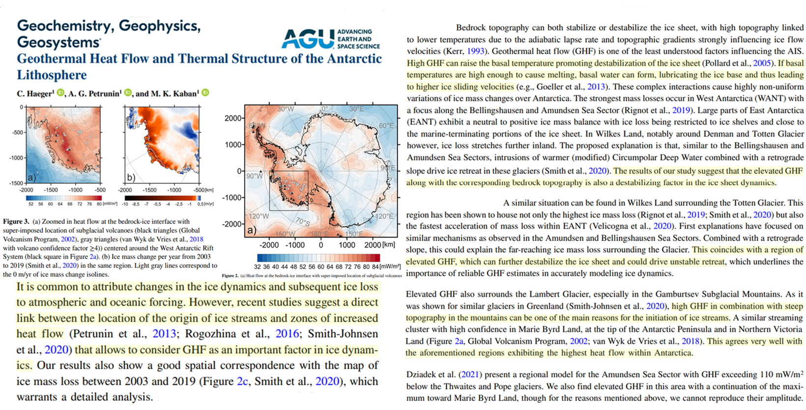
Anomalously High Heat Flow Regions Beneath the Transantarctic Mountains and Wilkes Subglacial Basin in East Antarctica Inferred From Curie Depth … The Transantarctic Mountains (TAMs) separate the warmer lithosphere of the Cretaceous-Tertiary West Antarctic rift system and the colder and older provinces of East Antarctica. Low velocity zones beneath the TAM imaged in recent seismological studies have been interpreted as warm low-density mantle material, suggesting a strong contribution of thermal support to the uplift of the TAM. We present new Curie Point Depth (CPD) and geothermal heat flow (GHF) maps of the northern TAM and adjacent Wilkes Subglacial Basin (WSB) based exclusively on high resolution magnetic airborne measurements. We find shallow CPD and high GHF beneath the northern TAM, reinforcing the hypothesis of thermal support of the topography of the mountain range. Additionally, this study demonstrates, that limiting spectral analysis to areas with a high density of aeromagnetic measurements increases the resolution of CPD estimates revealing localized shallow CPD and associated high heat flow in the Central Basin of the WSB and the Rennick Graben (RG).
It is common to attribute changes in the ice dynamics and subsequent ice loss to atmospheric and oceanic forcing. However, recent studies suggest a direct link between the location of the origin of ice streams and zones of increased heat flow (Petrunin et al., 2013; Rogozhina et al., 2016; Smith-Johnsen et al., 2020) that allows to consider GHF as an important factor in ice dynamics. Our results also show a good spatial correspondence with the map of ice mass loss between 2003 and 2019.
Glaciers, Ice Sheets, Sea Ice
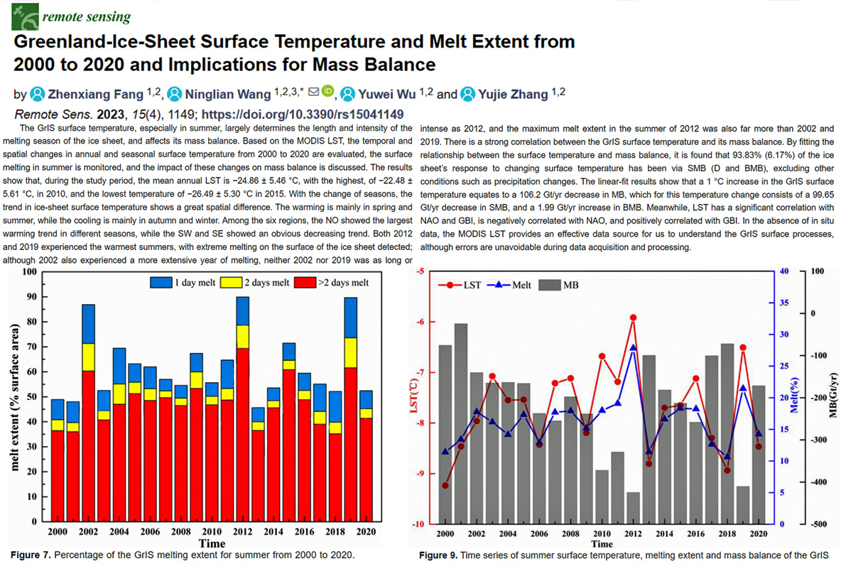
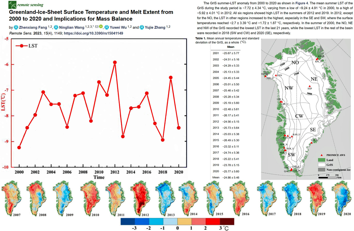
The GrIS surface temperature, especially in summer, largely determines the length and intensity of the melting season of the ice sheet, and affects its mass balance. Based on the MODIS LST, the temporal and spatial changes in annual and seasonal surface temperature from 2000 to 2020 are evaluated, the surface melting in summer is monitored, and the impact of these changes on mass balance is discussed. The results show that, during the study period, the mean annual LST is −24.86 ± 5.46 °C, with the highest, of −22.48 ± 5.61 °C, in 2010, and the lowest temperature of −26.49 ± 5.30 °C in 2015. With the change of seasons, the trend in ice-sheet surface temperature shows a great spatial difference. The warming is mainly in spring and summer, while the cooling is mainly in autumn and winter. Among the six regions, the NO showed the largest warming trend in different seasons, while the SW and SE showed an obvious decreasing trend.
The centennial response of land-terminating glaciers in Greenland to climate change is largely unknown. Yet, such information is important to understand ongoing changes and for projecting the future evolution of Arctic subpolar glaciers, meltwater runoff, and sediment fluxes. This paper analyses the topography, geomorphology, and sedimentology of prominent moraine ridges and the proglacial areas of ice cap outlet glaciers on the Qaanaaq peninsula (Piulip Nunaa). We determine geometric changes of glaciers since the neoglacial maximum; the Little Ice Age (LIA), and we compare glacier behaviour during the LIA with that of the present day. There has been very little change in the rate of volume loss of each outlet glacier since the LIA compared with the rate between 2000 and 2019.
During the warmest part of the Holocene, roughly 9–5 ka (Holocene Thermal Maximum, HTM), temperatures in the high latitudes were 1.5–2.5 °C higher, and Arctic sea ice area likely smaller than at present.
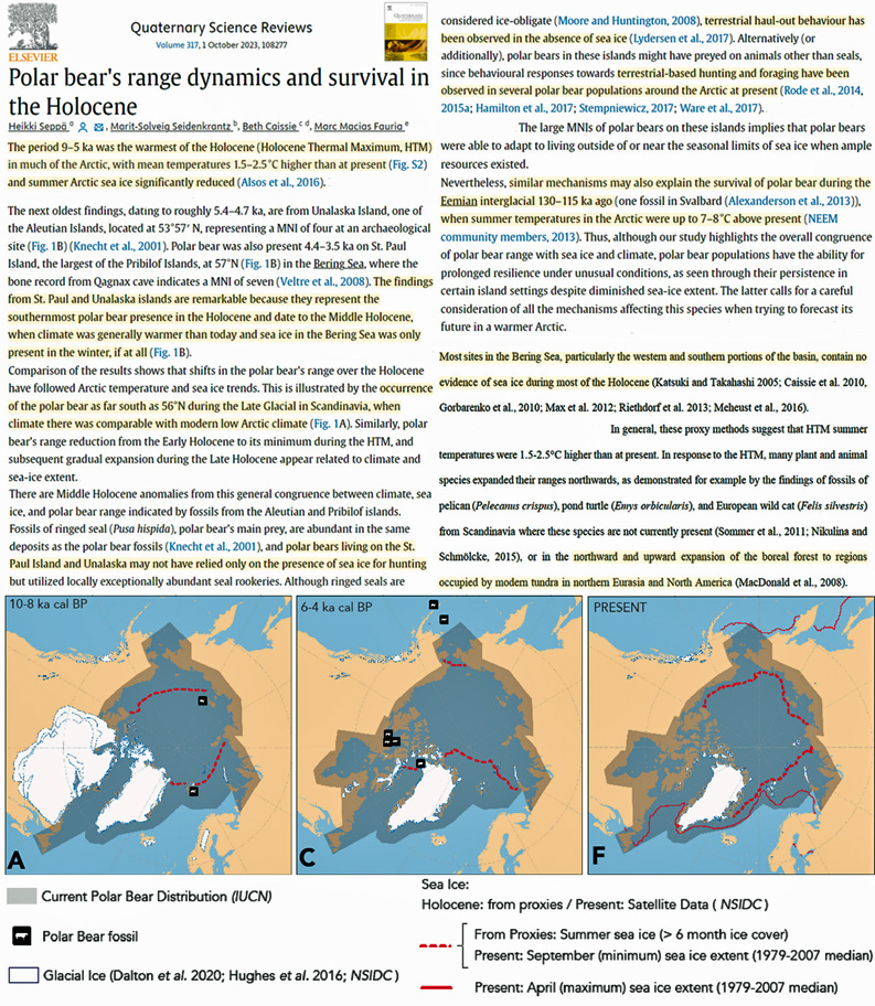
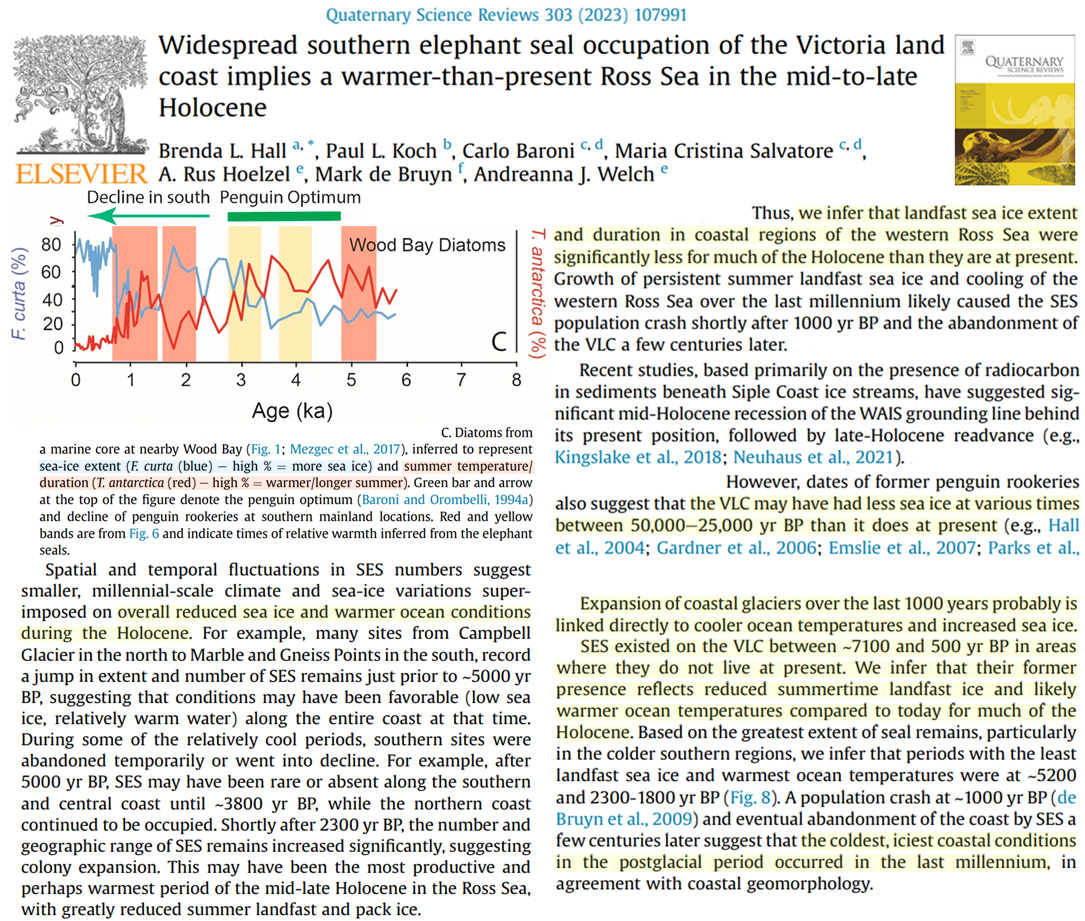
SES [southern elephant seals] existed on the VLC [Victoria Land Coast] between ~7100 and 500 yr BP in areas where they do not live at present. We infer that their former presence reflects reduced summertime landfast ice and likely warmer ocean temperatures compared to today for much of the Holocene. Based on the greatest extent of seal remains, particularly in the colder southern regions, we infer that periods with the least landfast sea ice and warmest ocean temperatures were at ~5200 and 2300-1800 yr BP (Fig. 8). A population crash at ~1000 yr BP (de Bruyn et al., 2009) and eventual abandonment of the coast by SES a few centuries later suggest that the coldest, iciest coastal conditions in the postglacial period occurred in the last millennium, in agreement with coastal geomorphology. … Expansion of coastal glaciers over the last 1000 years probably is linked directly to cooler ocean temperatures and increased sea ice. … [W]e infer that landfast sea ice extent and duration in coastal regions of the western Ross Sea were significantly less for much of the Holocene than they are at present. Growth of persistent summer landfast sea ice and cooling of the western Ross Sea over the last millennium likely caused the SES population crash shortly after 1000 yr BP and the abandonment of the VLC a few centuries later. … We infer that the documented population crash and abandonment of the entire coast by SES after ~1000-500 yr BP was due to return of heavy sea ice (particularly summer landfast ice), the greatest of the postglacial period, and likely cold ocean temperatures. We speculate that these conditions also may have resulted in contraction of the Cape Adare Adelie penguin “super colony” (Emslie et al., 2018), as well as the disappearance of this species at Cape Irizar (Emslie, 2021).
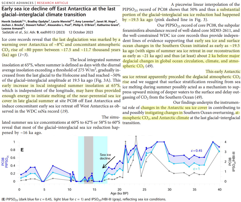
The local integrated summer insolation at 65°S, where summer is defined as days with the diurnal average insolation exceeding a threshold of 275 W/m2 , gradually increased from the last glacial to the Holocene and had reached ~50% of the glacial–interglacial amplitude at 19.5 ka ago (Fig. 3A). This early increase in local integrated summer insolation at 65°S, which is independent of the longitude, may have thus provided enough energy to initiate melting of the near-perennial sea ice cover in late glacial summer at site PC08 off East Antarctica and induce concomitant early sea ice retreat off West Antarctica as observed in the WDC ssNa record (19). … Our PIPSO25 record of core PC08, the subpolar foraminifera abundance record of well-dated core MD03-2611, and the well-constrained WDC ice core records thus provide independent lines of evidence supporting that early sea ice and surface ocean changes in the Southern Ocean initiated as early as ~19.5 ka ago (with signs of summer sea ice retreat in our reconstruction as early as ~21 ka ago) and thus (at least) about 2 ka before major deglacial changes in global ocean circulation, climate, and atmospheric CO2 … This early Antarctic sea ice retreat apparently preceded the deglacial atmospheric CO2 rise … Our findings underpin the instrumental role of changes in the Antarctic sea ice cover in contributing to and possibly instigating changes in Southern Ocean overturning, atmospheric CO2, and Antarctic climate at the last glacial–interglacial transition.
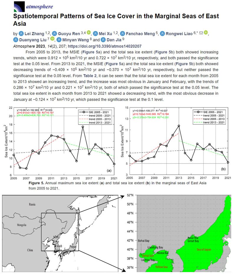
Over the past 17 years, the maximum sea ice extent in the marginal seas of East Asia reached a maximum value of 17.4 × 10⁴ km2 in 2016 and a minimum value of 7.6 × 10⁴ km2 in 2007. The sea ice extent of the marginal seas of East Asia from the 6th pentad in January to the 1st pentad in March was relatively large, resulting in the maximum of the total sea ice extent in 2013. The maximum sea ice extent and the total sea ice extent over the past 17 years had obvious differences in the change trend for the first and second halves of the period, and they all showed the change characteristics of first increasing and then decreasing. From 2005 to 2013, the trends in the maximum sea ice extent and the total sea ice extent were, respectively, 0.912 × 10⁵ km2/10 yr and 0.722 × 10⁷ km2/10 yr, which passed the significance test at the 0.05 level.
During the colder parts of the Holocene, temperature conditions likely were still warmer than at the Tron site today, which suggests persistently permafrost-free conditions
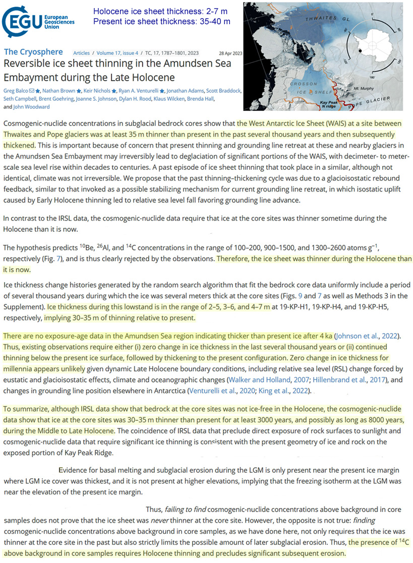
Cosmogenic-nuclide concentrations in subglacial bedrock cores show that the West Antarctic Ice Sheet (WAIS) at a site between Thwaites and Pope glaciers was at least 35 m thinner than present in the past several thousand years and then subsequently thickened. This is important because of concern that present thinning and grounding line retreat at these and nearby glaciers in the Amundsen Sea Embayment may irreversibly lead to deglaciation of significant portions of the WAIS, with decimeter- to meter-scale sea level rise within decades to centuries. A past episode of ice sheet thinning that took place in a similar, although not identical, climate was not irreversible. We propose that the past thinning–thickening cycle was due to a glacioisostatic rebound feedback, similar to that invoked as a possible stabilizing mechanism for current grounding line retreat, in which isostatic uplift caused by Early Holocene thinning led to relative sea level fall favoring grounding line advance. … There are no exposure-age data in the Amundsen Sea region indicating thicker than present ice after 4 ka
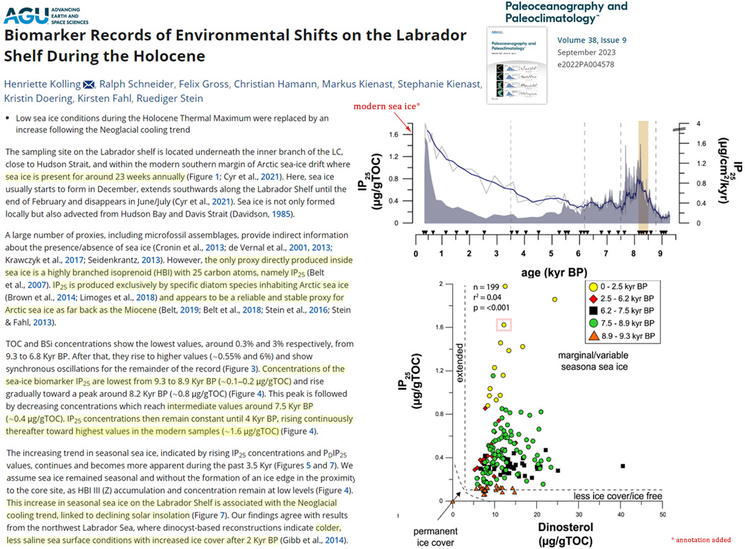
[Per a reliable sea ice biomarker proxy (IP25), the Labrador Sea ice was lowest (~0.1 μg/gTOC) 9.3-8.9k yrs ago and low (~0.4 μg/gTOC) 7.5-4k yrs ago. In contrast, modern sea ice lasts 23 weeks/yr and is the highest in 10k yrs (~1.6 μg/gTOC).]
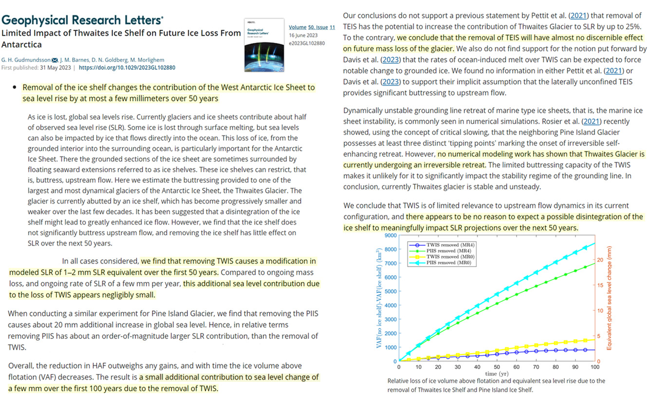
Here we estimate the buttressing provided to one of the largest and most dynamical glaciers of the Antarctic Ice Sheet, the Thwaites Glacier. The glacier is currently abutted by an ice shelf, which has become progressively smaller and weaker over the last few decades. It has been suggested that a disintegration of the ice shelf might lead to greatly enhanced ice flow. However, we find that the ice shelf does not significantly buttress upstream flow, and removing the ice shelf has little effect on SLR over the next 50 years. … Removal of the ice shelf changes the contribution of the West Antarctic Ice Sheet to sea level rise by at most a few millimeters over 50 years … In all cases considered, we find that removing TWIS causes a modification in modeled SLR of 1–2 mm SLR equivalent over the first 50 years. Compared to ongoing mass loss, and ongoing rate of SLR of a few mm per year, this additional sea level contribution due to the loss of TWIS appears negligibly small. … Directly upstream of the eastern sector of Thwaites’ grounding line, and approximately upstream of TEIS, removing TWIS causes an increase in ice thickness. Hence, over this area (shown in blue Figure 4a), removing TWIS causes, at least initially, a decrease in global sea level. … Overall, the reduction in HAF outweighs any gains, and with time the ice volume above flotation (VAF) decreases. The result is a small additional contribution to sea level change of a few mm over the first 100 years due to the removal of TWIS. … Our conclusions do not support a previous statement by Pettit et al. (2021) that removal of TEIS has the potential to increase the contribution of Thwaites Glacier to SLR by up to 25%. To the contrary, we conclude that the removal of TEIS will have almost no discernible effect on future mass loss of the glacier. We also do not find support for the notion put forward by Davis et al. (2023) that the rates of ocean-induced melt over TWIS can be expected to force notable change to grounded ice. We found no information in either Pettit et al. (2021) or Davis et al. (2023) to support their implicit assumption that the laterally unconfined TEIS provides significant buttressing to upstream flow. … [N]o numerical modeling work has shown that Thwaites Glacier is currently undergoing an irreversible retreat. … We conclude that TWIS is of limited relevance to upstream flow dynamics in its current configuration, and there appears to be no reason to expect a possible disintegration of the ice shelf to meaningfully impact SLR projections over the next 50 years.
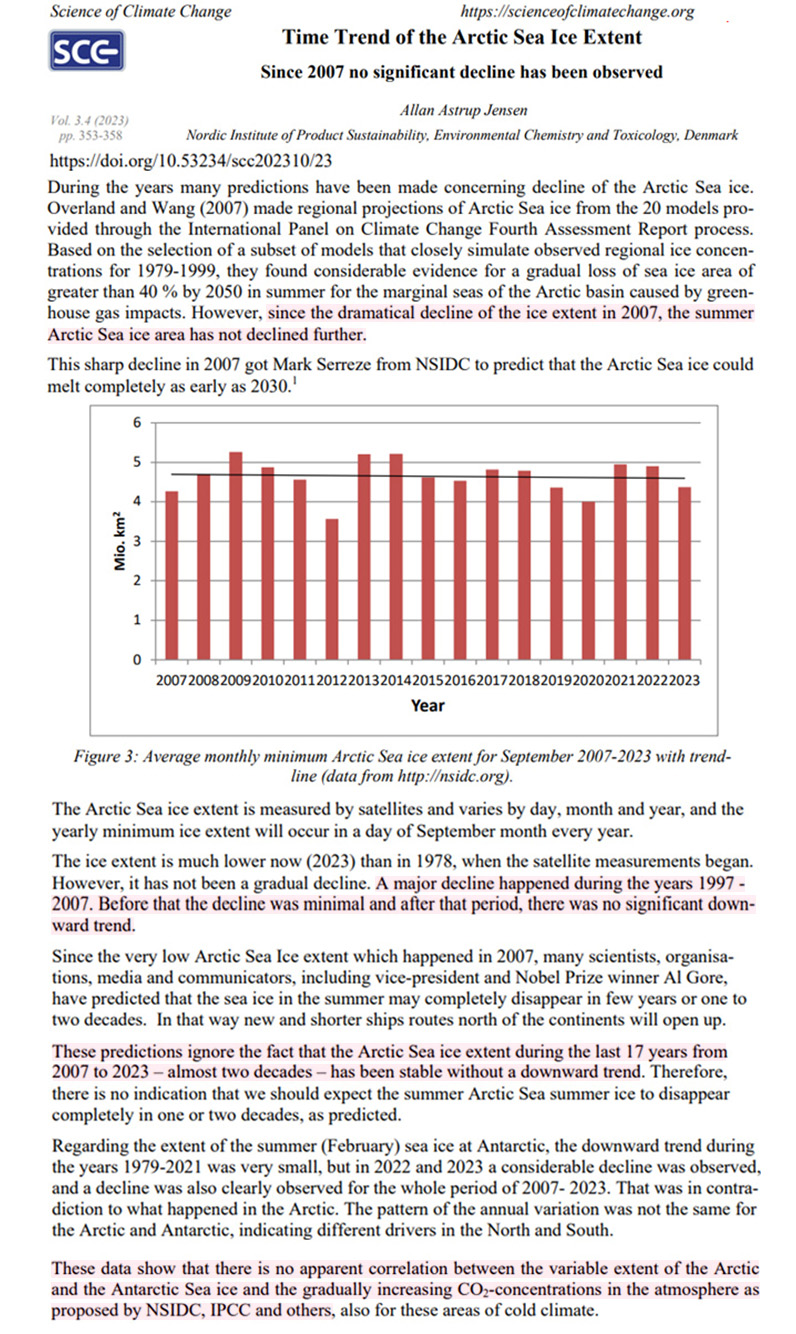
The Arctic Sea ice extent is measured by satellites and varies by day, month and year, and the yearly minimum ice extent will occur in a day of September month every year. The ice extent is much lower now (2023) than in 1978, when the satellite measurements began. However, it has not been a gradual decline. A major decline happened during the years 1997 – 2007. Before that the decline was minimal and after that period, there was no significant downward trend. … These data show that there is no apparent correlation between the variable extent of the Arctic and the Antarctic Sea ice and the gradually increasing CO2-concentrations in the atmosphere as proposed by NSIDC, IPCC and others, also for these areas of cold climate.
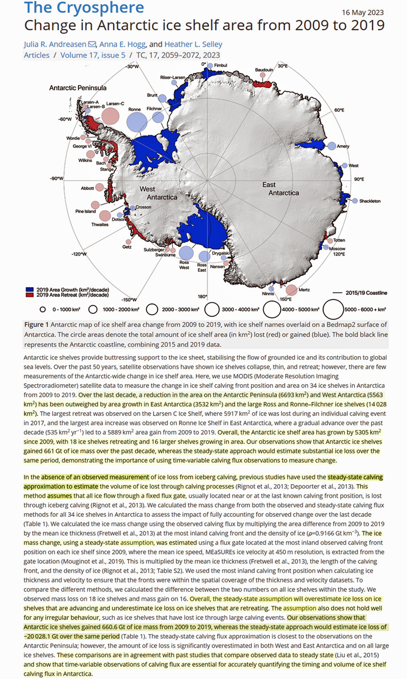
Here, we use MODIS (Moderate Resolution Imaging Spectroradiometer) satellite data to measure the change in ice shelf calving front position and area on 34 ice shelves in Antarctica from 2009 to 2019. Over the last decade, a reduction in the area on the Antarctic Peninsula (6693 km2) and West Antarctica (5563 km2) has been outweighed by area growth in East Antarctica (3532 km2) and the large Ross and Ronne–Filchner ice shelves (14 028 km2). The largest retreat was observed on the Larsen C Ice Shelf, where 5917 km2 of ice was lost during an individual calving event in 2017, and the largest area increase was observed on Ronne Ice Shelf in East Antarctica, where a gradual advance over the past decade (535 km2 yr−1) led to a 5889 km2 area gain from 2009 to 2019. Overall, the Antarctic ice shelf area has grown by 5305 km2 since 2009, with 18 ice shelves retreating and 16 larger shelves growing in area. Our observations show that Antarctic ice shelves gained 661 Gt of ice mass over the past decade, whereas the steady-state approach would estimate substantial ice loss over the same period, demonstrating the importance of using time-variable calving flux observations to measure change. … Overall, the steady-state assumption will overestimate ice loss on ice shelves that are advancing and underestimate ice loss on ice shelves that are retreating. The assumption also does not hold well for any irregular behaviour, such as ice shelves that have lost ice through large calving events. Our observations show that Antarctic ice shelves gained 660.6 Gt of ice mass from 2009 to 2019, whereas the steady-state approach would estimate ice loss of −20 028.1 Gt over the same period.
It seems clear that all glaciers in the Polar Urals must have melted away soon after the onset of the Holocene when the climate suddenly became significantly warmer than today, suggesting that it was impossible for glaciers to exist even in shady high-elevation locations.
Solar Influence On Climate
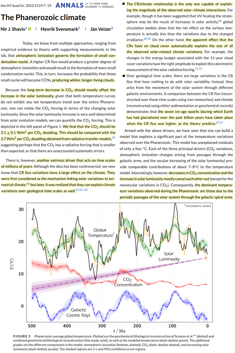
The CR/climate relationship is the only one capable of explaining the magnitude of the observed solar-climate interactions. … The apparent effect that the CRs have on cloud cover automatically explains the size of all the observed solar-related climate variations. … The seven ice-age epochs…over the past billion years have taken place when the CR flux was higher, as the theory predicts. … Decreases in CO2 concentration and the increase in solar luminosity mostly cancel each other out.
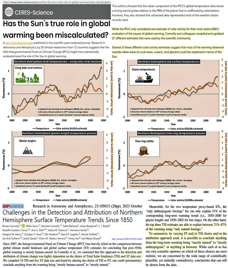
The rural and urban blend indicates a long-term warming of 0.89°C/century since 1850, while the rural-only temperature indicates 0.55°C/century. This contradicts the common assumption that current thermometer based global temperature indices are relatively unaffected by urban warming biases. … The other TSI time series was apparently overlooked by IPCC AR6. It was found that altering the temperature estimate and/or the choice of solar forcing dataset resulted in very different conclusions as to the primary drivers of the observed warming. … Meanwhile, we found that simply substituting an alternative solar forcing dataset to that considered by AR6’s climate model hindcasts can substantially increase the amount of the 1850-2018 warming that can be explained in terms of natural forcing…87% of the “rural-only” temperature series.
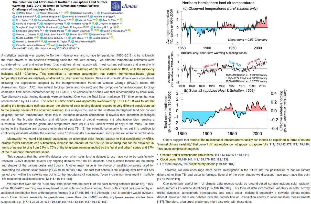
To summarize, by varying ST and/or TSI choice and/or the attribution approach used, it is possible to conclude anything from the long-term warming being “mostly natural” to “mostly anthropogenic” or anything in between. While each of us has our own scientific opinions on which of these choices are most realistic, we are concerned by the wide range of scientifically plausible, yet mutually contradictory, conclusions that can still be drawn from the data.
Several of these different solar activity estimates suggest that most of the warming observed outside urban areas (in rural areas, oceans, and glaciers) could be explained in terms of the Sun.
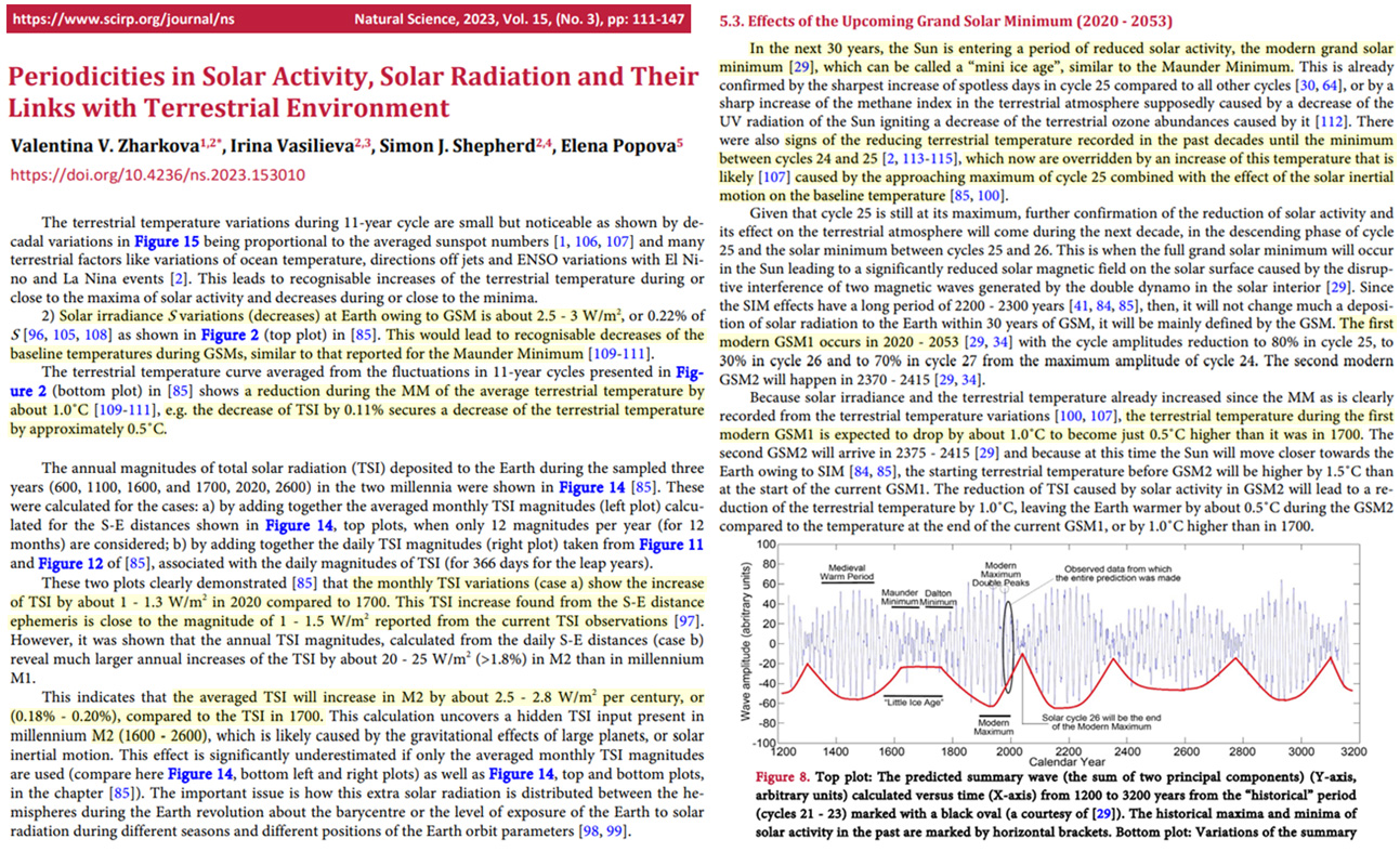
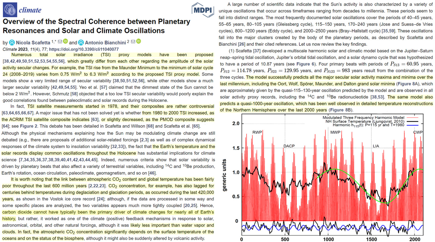
Given that cycle 25 is still at its maximum, further confirmation of the reduction of solar activity and its effect on the terrestrial atmosphere will come during the next decade, in the descending phase of cycle 25 and the solar minimum between cycles 25 and 26. This is when the full grand solar minimum will occur in the Sun leading to a significantly reduced solar magnetic field on the solar surface caused by the disruptive interference of two magnetic waves generated by the double dynamo in the solar interior [29]. Since the SIM effects have a long period of 2200 – 2300 years [41 , 84 , 85], then, it will not change much a deposition of solar radiation to the Earth within 30 years of GSM, it will be mainly defined by the GSM. The first modern GSM1 occurs in 2020 – 2053 [29 , 34] with the cycle amplitudes reduction to 80% in cycle 25, to 30% in cycle 26 and to 70% in cycle 27 from the maximum amplitude of cycle 24. The second modern GSM2 will happen in 2370 – 2415 [29 , 34]. … Because solar irradiance and the terrestrial temperature already increased since the MM as is clearly recorded from the terrestrial temperature variations [100 , 107], the terrestrial temperature during the first modern GSM1 is expected to drop by about 1.0˚C to become just 0.5˚C higher than it was in 1700. The second GSM2 will arrive in 2375 – 2415 [29] and because at this time the Sun will move closer towards the Earth owing to SIM [84 , 85], the starting terrestrial temperature before GSM2 will be higher by 1.5˚C than at the start of the current GSM1. The reduction of TSI caused by solar activity in GSM2 will lead to a reduction of the terrestrial temperature by 1.0˚C, leaving the Earth warmer by about 0.5˚C during the GSM2 compared to the temperature at the end of the current GSM1, or by 1.0˚C higher than in 1700.
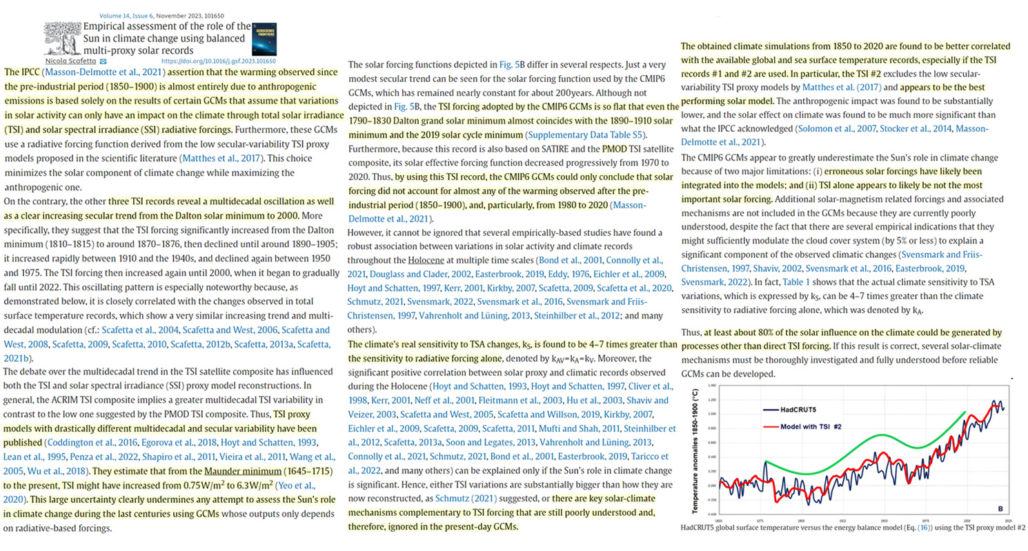
If the solar record by Matthes et al. (2017) is replaced with the three proposed balanced TSI forcing functions (see Fig. 4), and these functions are assumed to be proxies for TSA changes that can influence the climate in various (known and unknown) ways, the proposed modeling suggests that the solar total impact on the climate could be 4–7 times greater than its TSI effect alone. … Thus, at least about 80% of the solar influence on the climate could be generated by processes other than direct TSI forcing. If this result is correct, several solar-climate mechanisms must be thoroughly investigated and fully understood before reliable GCMs can be developed.
Climate/Precipitation Natural Variability
In recent years, the Southern Ocean has experienced unprecedented surface warming and sea ice loss—a stark reversal of the sea ice expansion and surface cooling that prevailed over the preceding decades. Here, we examine the mechanisms that led to the abrupt circumpolar surface warming events that occurred in late 2016 and 2019 and assess the role of internal climate variability. A mixed layer heat budget analysis reveals that these recent circumpolar surface warming events were triggered by a weakening of the circumpolar westerlies, which decreased northward Ekman transport and accelerated the seasonal shoaling of the mixed layer. We emphasize the underappreciated effect of the latter mechanism, which played a dominant role and amplified the warming effect of air–sea heat fluxes during months of peak solar insolation. An examination of the CESM1 large ensemble demonstrates that these recent circumpolar warming events are consistent with the internal variability associated with the Southern Annular Mode (SAM), whereby negative SAM in austral spring favors shallower mixed layers and anomalously high summertime SST. A key insight from this analysis is that the seasonal phasing of springtime mixed layer depth shoaling is an important contributor to summertime SST variability in the Southern Ocean. Thus, future Southern Ocean summertime SST extremes will depend on the coevolution of mixed layer depth and surface wind variability.
The composite time series of daily rainfall for Brisbane from 1860 to 2022 shows evidence of natural oscillations and the absence of any growing or reducing trend. The linear trend has a slope of only -2 μm/year, which is statistically insignificant. Similarly insignificant is the acceleration, calculated as double the 2nd order coefficient of the parabolic trend, at +0.02 μm/year2. Higher than February 2022 single-day rainfall, three-day consecutive rainfall, or single-month rainfall, were measured in the past. The natural oscillations have, amongst others, clear inter-annual, decadal, and multi-decadal cycles, of lengths slightly less than 10, about 20, about 40, and 65-80 years (quasi-60 years). We conclude that the climate for south-eastern Queensland is characterised by a fairly stable rainfall pattern, dominated by wet and dry cycles.
The analysis showed that the annual variability of temperature over Europe was mainly influenced by natural processes, the variability of which explains ~65% of its variance. Radiative forcing, which is a function of anthropogenic increase in CO2 concentration in the atmosphere, explains only 7–8% of the variability of the average annual temperature over Europe, being a secondary or tertiary factor in shaping its changes.
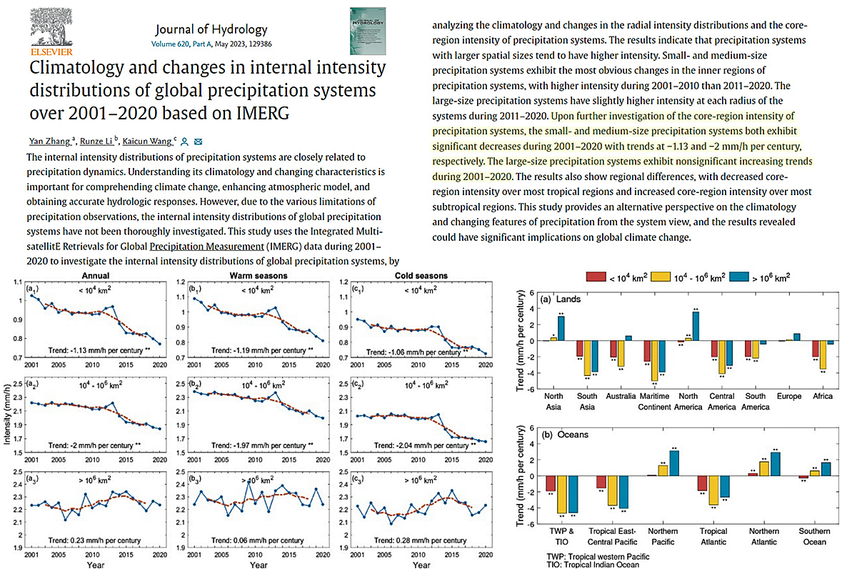
The internal intensity distributions of precipitation systems are closely related to precipitation dynamics. Understanding its climatology and changing characteristics is important for comprehending climate change, enhancing atmospheric model, and obtaining accurate hydrologic responses. However, due to the various limitations of precipitation observations, the internal intensity distributions of global precipitation systems have not been thoroughly investigated. This study uses the Integrated Multi-satellitE Retrievals for Global Precipitation Measurement (IMERG) data during 2001–2020 to investigate the internal intensity distributions of global precipitation systems, by analyzing the climatology and changes in the radial intensity distributions and the core-region intensity of precipitation systems. The results indicate that precipitation systems with larger spatial sizes tend to have higher intensity. Small- and medium-size precipitation systems exhibit the most obvious changes in the inner regions of precipitation systems, with higher intensity during 2001–2010 than 2011–2020. The large-size precipitation systems have slightly higher intensity at each radius of the systems during 2011–2020. Upon further investigation of the core-region intensity of precipitation systems, the small- and medium-size precipitation systems both exhibit significant decreases during 2001–2020 with trends at −1.13 and −2 mm/h per century, respectively. The large-size precipitation systems exhibit nonsignificant increasing trends during 2001–2020. The results also show regional differences, with decreased core-region intensity over most tropical regions and increased core-region intensity over most subtropical regions.
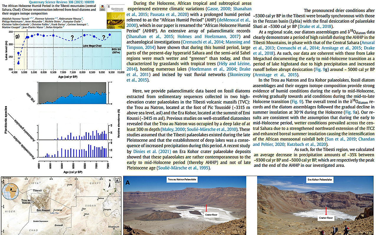
During the Holocene, African tropical and subtropical areas experienced extreme climate variations. … [L]arge parts of the present-day hyperarid Sahara…were much wetter and “greener” than today. … Here, we provide palaeoclimatic data based on fossil diatoms extracted from sedimentary sequences collected in two high-elevation crater palaeolakes in the Tibesti volcanic massifs (TVC): the Trou au Natron, located at the foot of Pic Toussidé (∼3315 m above sea level, asl) and the Era Kohor, located at the summit of Emi Koussi (∼3415 m asl). Previous studies on well-stratified diatomites revealed that the Trou au Natron was occupied by a deep lake of at least 300 m depth (Maley, 2000; Soulié-Märsche et al., 2010). These studies assumed that the Tibesti palaeolakes existed during the late Pleistocene and that the establishment of deep lakes was a consequence of increased precipitation during this period. A recent study by Dinies et al. (2021) on Era Kohor crater palaeolake deposits showed that these palaeolakes are rather contemporaneous to the early to mid-Holocene period (thereby AHHP) and not of late Pleistocene age (Soulié-Märsche et al., 1995).
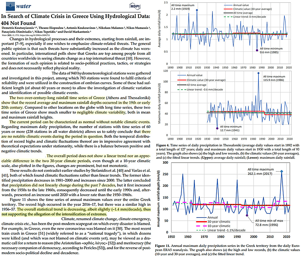
The two over-century-long rainfall time series of Greece (Athens and Thessaloniki) show that the record average and maximum rainfall depths occurred in the 19th or early 20th century. Compared to other locations on the globe with long time series, these two time series of Greece show much smaller to negligible climate variability, both in mean and maximum rainfall heights. … The overall statistical trend is decreasing, albeit slightly (–1.4 mm/decade), thus not supporting the allegation of the intensification of extremes. … Climate, renamed climate change, climate emergency, climate crisis etc., has been the post-modern scapegoat on which every disaster is blamed. For example, in Greece, even the new coronavirus was blamed on it [50]. The most recent train crash in Greece [51] (widely referred to as a “national tragedy”), in which dozens were killed (and which was not blamed on climatic events yet), may be viewed as a dramatic call for a return to reason (the Aristotelian «ορθός λόγος» [52]) and meritocracy (the necessary companion of democracy, according to Pericles [53]), and for the reverse of postmodern socio-political decline and decadence. … Changes in hydrological processes and their extremes, starting from rainfall, are important [7–9], especially if one wishes to emphasize climate-related threats. The general public opinion is that such threats have substantially increased as the climate has worsened. In particular, international polls show that Greeks are top among people from all countries worldwide in seeing climate change as a top international threat [10]. However, the formation of such opinion is related to socio-political practices, tactics, or strategies and does not necessarily reflect physical reality.
Cloud/Aerosol Climate Influence
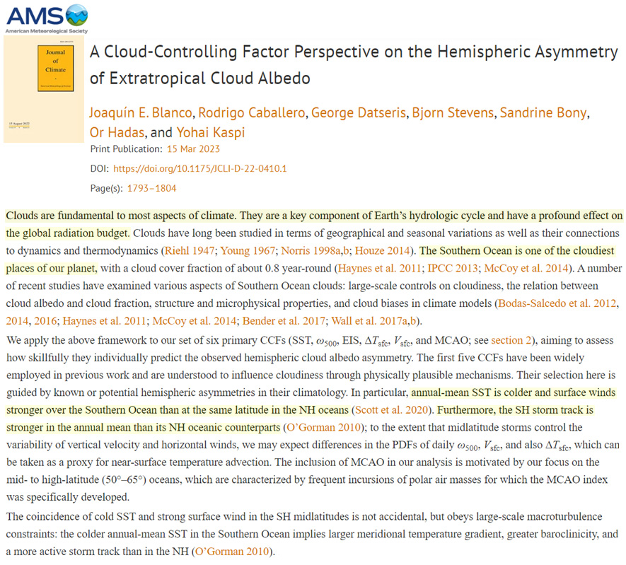
Clouds are fundamental to most aspects of climate. They are a key component of Earth’s hydrologic cycle and have a profound effect on the global radiation budget. … [T]he colder annual-mean SST in the Southern Ocean implies…a more active storm track than in the NH (O’Gorman 2010).
Clouds are a critical atmospheric constituent in regulating earth’s energy budget (controlling the global temperature) by reflecting incident sunlight (a cooling effect), and emitting radiation to the ground (warming below clouds) and to space. The net warming or cooling effect of these factors is called the cloud radiative effect (CRE). The CRE varies with ordinary climate oscillations such as the well-known El Niño-Southern Oscillation (ENSO), and may amplify or partly suppress long-term global warming depending on whether cloud cover diminishes or increases. This study tests a way to summarize global cloud property variations, observed in great detail by satellites, in terms of various two-dimensional characteristic patterns defined by the spherical harmonic functions. For example, ENSO variations can be clearly observed in one of the characteristic patterns of CRE changes.
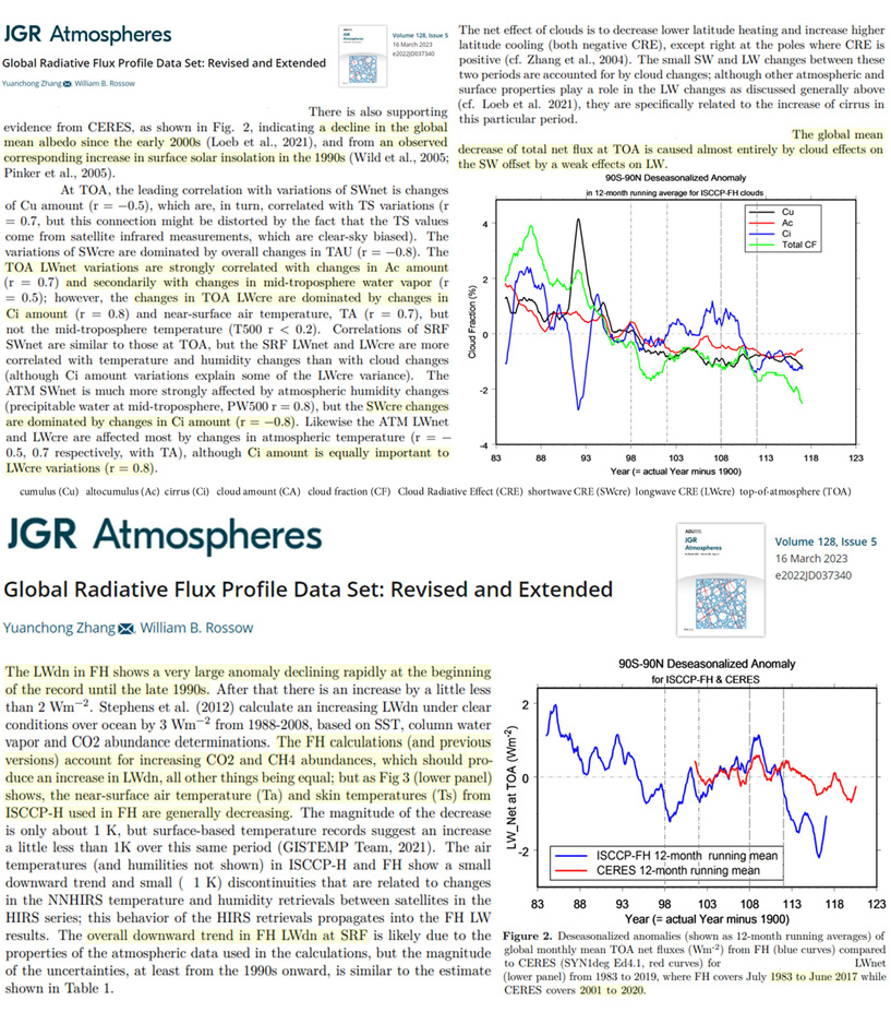
The LWdn [longwave net at TOA (W/m²)] shows a very large anomaly declining rapidly at the beginning of the record until the late 1990s. … The FH calculations (and previous versions) account for increasing CO2 and CH4 abundances, which should produce an increase in LWdn, all other things being equal; but as Fig 3…shows, the near surface air temperature (Ta) and skin temperatures (Ts) from ISCCP-H used in FH are generally decreasing. … [July 1983 to June 2017] overall downward trend in FH LWdn [longwave net at TOA (W/m²)]
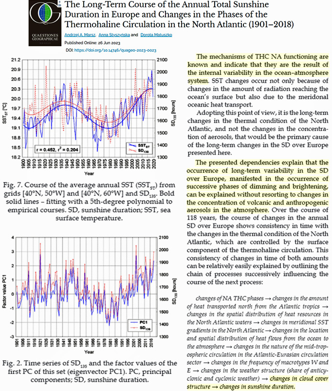
The mechanisms of the THC NA functioning are known and indicate that they are the result of the internal variability in the ocean-atmosphere system. … SST changes occur not only because of changes in the amount of radiation reaching the ocean’s surface but also due to the meridonal oceanic heat transport. … [I]t is the long-term changes in the thermal condition of the North Atlantic, and not changes in the concentration of aerosols, that would be the primary cause of the long-term change in the SD over Europe. … [T]he occurrence of long-term variability in the SD over Europe, manifested in the occurrence of successive phases of dimming and brightening, can be explained without resorting to changes in the concentration of volcanic and anthropogenic aerosols in the atmosphere.
In summary, demasking the aerosol-induced surface cooling through climate mitigation actions will unveil the actual magnitude and effect of GHG-induced global warming; we shall anticipate a decades-long transitory increase in surface temperatures from planned mitigations. … The major surprise from the study is the magnitude of the COVID shutdown-induced increase in surface-reaching solar radiation, the surface brightening, of the order of 15–20 W m−2. This surface brightening has major implications for the regional climate, especially the monsoonal circulation39, atmospheric circulation, and precipitation over SA, and likely also for East Asia and all tropical regions. Other recent studies also reported weakening of the aerosol cooling effect due to the Covid-19 lockdown and a subsequent short-term warming effect. … Mitigation strategies focusing on the phase-out of fossil fuels will lead to quick removal of the short-lived aerosols while the longer-lived major greenhouse gases decrease much more slowly, likely resulting in undesired net warming of the climate during a decades-long transition period.

The CO2 Greenhouse Effect – Climate Driver?
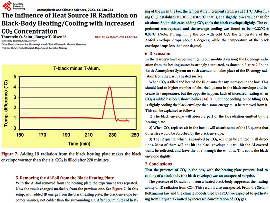
This study deals with interactions between thermal and radiative energy flow in experimental situations of varying complexity. Of special interest is how IR energy, re-emitted from CO2 gas, behaves in an earth/atmosphere simulated setup. Such an experiment was performed by Hermann Harde and Michael Schnell where they show that IR radiation emitted from CO2 can warm a small black-body metal plate. In a control experiment, we verified this result. However, in their experiment, the amount of IR radiation from the heating element was strongly attenuated. In a modified experiment, where IR emission from the heating source is present, no heating but a slight cooling of a black object is found when air is replaced by CO2. The modified experimental situation is also more like the earth/atmosphere situation.
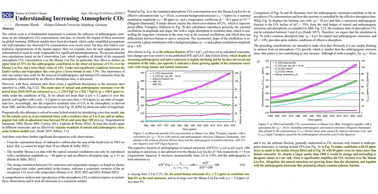
The carbon cycle is of fundamental importance to estimate the influence of anthropogenic emissions on the atmospheric CO2 concentration, and thus, to classify the impact of these emissions on global warming. Different models have been developed, which under simplified assumptions can well reproduce the observed CO2 concentration over recent years, but they also lead to contradictory interpretations of the human impact. Here we consider, how far such suppositions are substantiated or must be made responsible for significant misinterpretations. We present detailed own calculations based on the Conservation Law, which reproduce all details of the measured atmospheric CO2 concentration over the Mauna Loa Era. In particular, they allow to deduce an upper limit of 35% for the anthropogenic contribution to the observed increase of CO2 over the Mauna Loa Era, and a more likely value of 14%. Under non-equilibrium conditions between the Earth’s surface and troposphere this even gives a lower bound of only 3.5%.
All these categories are distinguished by focusing exclusively on changing anthropogenic emissions, while natural emissions in advance are excluded or are supposed to form a closed cycle. Under these conditions is the right-hand side of (2) not really the net of all natural fluxes, but represents the anthropogenic absorption rate. It is obvious that under such assumptions native emissions cannot have any impact. A conclusion that there is zero contribution from natural sources and sinks to the increase in the atmosphere, is no more and no less circular reasoning. … As elaborately discussed in Harde (2023), a realistic absorption rate, which is in agreement with all observations and physical principles, is scaling proportional to the instantaneous CO2 concentration and does not discriminate between native or anthropogenic emissions. … [Natural emissions rates can be calculated to add] 31.2 ppmv/yr to the increase, which is almost 6 times more than the human emissions.
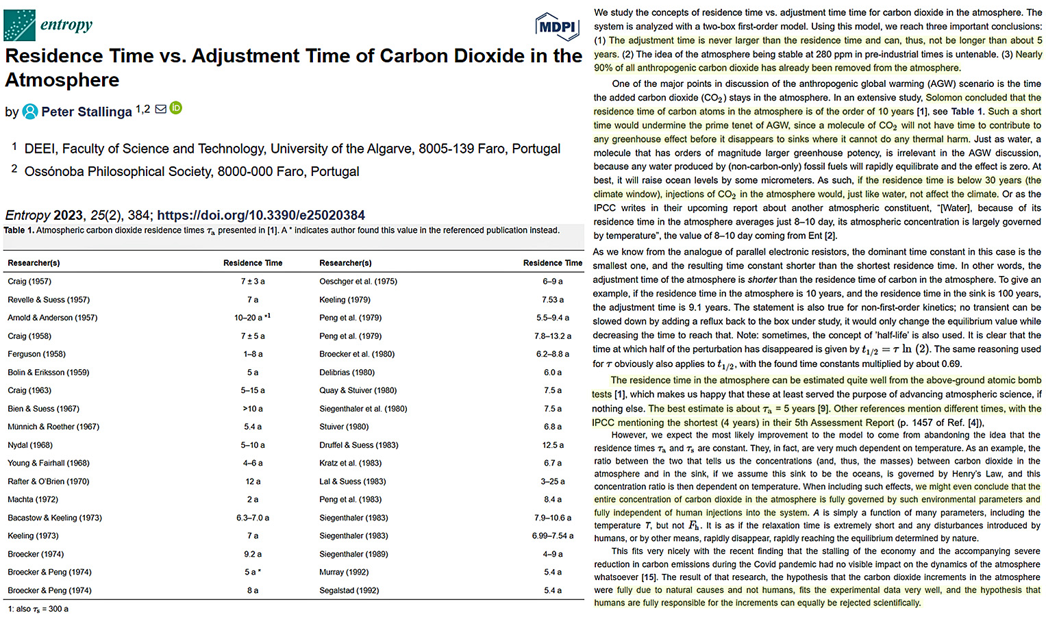
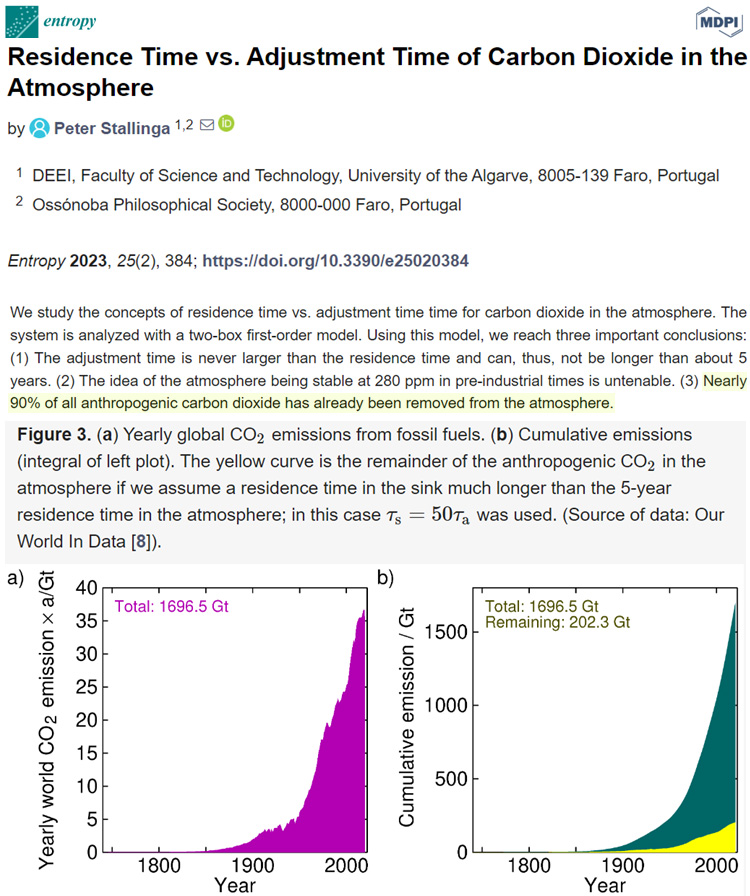
We study the concepts of residence time vs. adjustment time time for carbon dioxide in the atmosphere. The system is analyzed with a two-box first-order model. Using this model, we reach three important conclusions: (1) The adjustment time is never larger than the residence time and can, thus, not be longer than about 5 years. (2) The idea of the atmosphere being stable at 280 ppm in pre-industrial times is untenable. (3) Nearly 90% of all anthropogenic carbon dioxide has already been removed from the atmosphere.
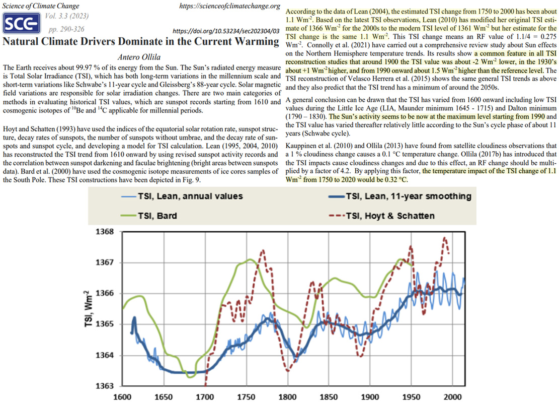
It is worth noting that the link between atmospheric CO2 content and global temperature has been fairly poor throughout the last 600 million years [2,22,23]. CO2 concentration, for example, has also lagged for centuries behind temperatures during deglaciation and glaciation periods, as occurred during the last 420,000 years, as shown in the Vostok ice core record [24]; although, if the data are processed in some way and some specific places are analyzed, the two variables appears much more tightly coupled [20,25]. Hence, carbon dioxide cannot have typically been the primary driver of climate changes for nearly all of Earth’s history, but rather, it worked as one of the climate (positive) feedback mechanisms in response to solar, astronomical, orbital, and other natural forcings, although it was likely less important than water vapor and clouds. In fact, the atmospheric CO2 concentration significantly depends on the surface temperature of the oceans and on the status of the biosphere, although it might also be suddenly altered by volcanic activity. … Indeed, numerous criteria show that solar variability is driven by planetary beats that also affect a variety of terrestrial variables, including 14C and 10Be production, Earth’s rotation, ocean circulation, paleoclimate, geomagnetism, and so on … Numerous total solar irradiance (TSI) proxy models have been proposed [38,42,49,50,51,52,53,54,55,56], which greatly differ from each other regarding the amplitude of the solar activity secular changes. For example, the TSI rise from the Maunder Minimum to the minimum of solar cycle 24 (2008–2019) varies from 0.75 W/m2 to 6.3 W/m2 according to the proposed TSI proxy model.
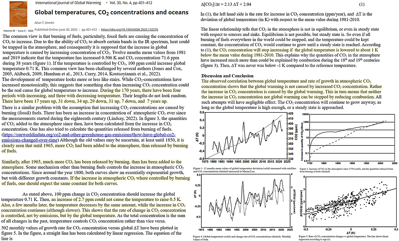
The observed correlation between global temperature and rate of growth in atmospheric CO2 concentration shows that the global warming is not caused by increased CO2 concentration. Rather the increase in CO2 concentration is caused by the global warming. This in turn means that neither the increase in CO2 concentration nor global warming can be stopped by reducing combustion. …the rate of change in CO2 concentration is controlled, not by emissions, but by the global temperature.
Incidents deemed examples of “climate change” such as forest fires, cyclones, floods, droughts, rising sea levels, coral bleaching, or variations polar ice coverage have no direct link with coal. They are all the result of variations in temperature. Coal is seen as a major contributor to the growth of carbon dioxide in the Earth’s atmosphere and, as carbon dioxide is a greenhouse gas which contributes to keeping the planet warm, the growing use of coal is blamed as a primary cause for the rise in global temperatures since the start of the Industrial Age around 1850. This chapter discusses various scientific facts which show that this supposed causal link between increasing levels of carbon dioxide and growing temperature is not correct at the current levels of atmospheric carbon dioxide. Furthermore, history has shown that the cyclic behavior in temperature over the past 170 years, over the past 10,000 years of the current Holocene interglacial, or over the millions of years of geological time, is not due to any such behavior of atmospheric carbon dioxide. The evidence shows that current rise in temperature is simply the result of a repeat of the millennial warm period cycle and thus has nothing to do with the use of coal.
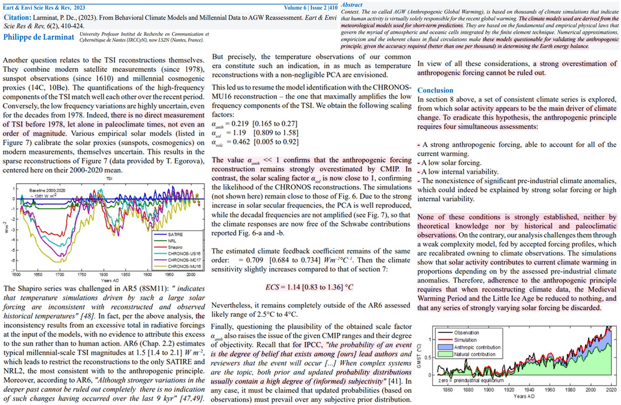
The estimated climate feedback coefficient remains of the same order: = 0.709 [0.684 to 0.734] Wm–2°C–1. Then the climate sensitivity [to doubled CO2] slightly increases compared to that of section 7: ECS = 1.14 [0.83 to 1.36] °C. Nevertheless, it remains completely outside of the AR6 assessed likely range of 2.5°C to 4°C.
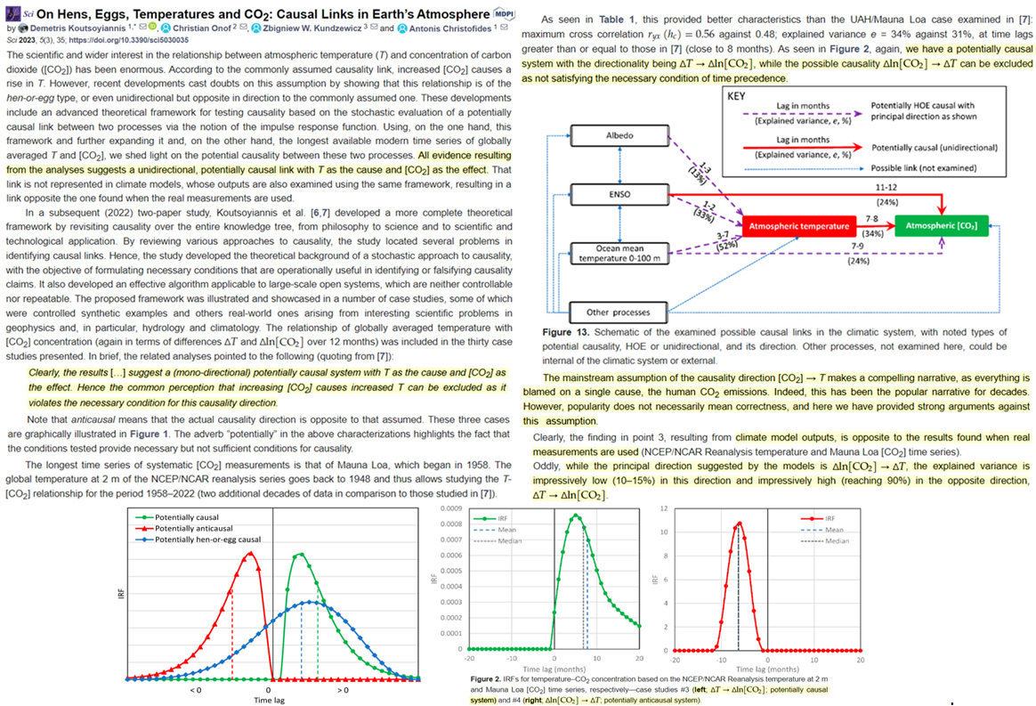
The mainstream assumption of the causality direction [CO2] → T makes a compelling narrative, as everything is blamed on a single cause, the human CO2 emissions. Indeed, this has been the popular narrative for decades. However, popularity does not necessarily mean correctness, and here we have provided strong arguments against this assumption. … Clearly the results […] suggest a (mono-directional) potentially causal system with T as the cause and [CO₂] as the effect. Hence the common perception that increasing [CO₂] causes increased T can be excluded as it violates the necessary condition for this causality direction. … All evidence resulting from the analyses suggests a unidirectional, potentially causal link with T [temperature] as the cause and [CO₂] as the effect.
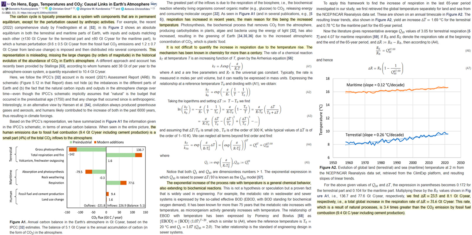
Beck’s historical data compilation consists of 97,404 samples of atmospheric CO2 mixing ratios,which were derived from 901 stations and cover a period from 1826 to 2008. The data show a pronounced maximum between 1939 and 1943 with a concentration up to 383 ppm, this in contrast to the monotonically rising CO2-levels reconstructed from ice cores. Alone the data aroundthis maximum from 1930 to 1950 represent about 60,000 samples and are based on the work of more than 25 different authors and locations. … Comparison with the historical CO2 data(Dark Dots) shows that the calculation confirms an increased emission and mixing ratio over the 30s to 50s, only with a broader and reduced maximum than the CO2 observations. Also the observed increasing concentration over the Mauna Loa Era (Light Blue Dots) can well be reproduced by the thermally induced emissions, while the anthropogenic emissions over this period will not contribute more than […] 12 ppmv (assuming equilibrium).
This study develops a very simple climate model, based on the standard lagging formula. The mathematical function is derived in detail. The main purpose is to estimate the e-time of carbon dioxide in the atmosphere. Many models evaluate the inflow to the atmospheric CO2 reservoir by rate equations describing the flow from e.g. sea to atmosphere with the weakness that not all parameters describing that flow are well known. This paper calculates the inflow and outflow to the atmosphere from the best data material that could be obtained. The conclusions are based on data rather than estimated flow parameters. I obtain as a result for each individual year an e-time. The average over 270 years is 3.96 years and it is fairly constant over this time period. A challenge in the compilation of the annual mass balance of CO2 in the atmosphere is the unknown amount of additional natural CO2 emission beyond the 1750 level. I used the amount determined by Skrable, and I add the increased emissions of the oceans due to temperature increase and the massive increase in wood burning to obtain a diagram that corresponds to the measured values of the CO2 increase. The conclusion is, that the anthropogenic contribution to atmospheric carbon dioxide in 2020 is only 28.9 ppmv. Including the anthropogenic burning of wood gives a total of 50.5 ppmv. I have estimated the Revelle factor (R) per year over 120 years. With an average value of 1.44, it is significantly lower than the value assumed by the IPCC. Thus, the absorptive capacity of the ocean is significantly higher than assumed in most IPCC models, where they use a Revelle factor (R) greater than 10. Also, the extent of biomass growth can be verified. All necessary data to falsify this are available in extensive databases.
Khmelinskii and Woodcock, 2023
The greenhouse gas hypothesis is based upon conjectures regarding the molecular spectroscopic properties of the CO2 molecule that may have never been validated. Here, we summarise some essential experimental facts regarding molecular physics of CO2 spectroscopy. The rate of emission of the photonic energy from the Earth’s surface as black body radiation by Stefan-Boltzmann law in the absorption bands of CO2 is limited compared to the [CO2] concentration capacity to absorb it [16,17]. In the IR spectra of CO2, the lines in the rotational structure of CO2 vibrational bands efficiently absorb about 10% of all IR in the specific IR bands where these lines appear, letting through the remaining 90%, and evidently absorbing absolutely nothing at all other IR wavelengths. Therefore, CO2 can affect no more than 10% of the surface-emitted IR radiation, and this absorption is already strongly saturated, as the absorption length does not exceed 300 meters for the relevant lines considered, whereas the troposphere, that determines climates, is 10 km thick.
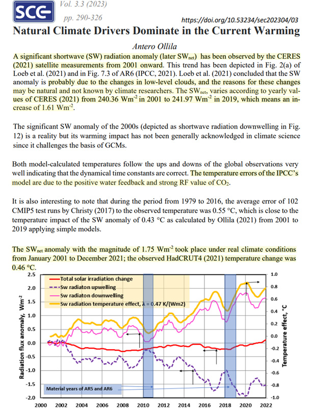
The alternative climate model NAGW including natural and anthropogenic drivers can explain the long-term global warming from 1750 onward as well the short-term warming during the 2000s. … The warming mechanisms of TSI and AHR include cloudiness changes and these quantitative effects are based on empirical temperature changes. This review concludes that the NAGW has a solid theoretical background, and its warming value has better conformity with the observed temperature than the AGW. … A significant shortwave (SW) radiation anomaly (later SWnet) has been observed by the CERES (2021) satellite measurements from 2001 onward. This trend has been depicted in Fig. 2(a) of Loeb et al. (2021) and in Fig. 7.3 of AR6 (IPCC, 2021). Loeb et al. (2021) concluded that the SW anomaly is probably due to the changes in low-level clouds, and the reasons for these changes may be natural and not known by climate researchers. The SWnet, varies according to yearly values of CERES (2021) from 240.36 Wm-2 in 2001 to 241.97 Wm-2 in 2019, which means an increase of 1.61 Wm-2. The significant SW anomaly of the 2000s (depicted as shortwave radiation downwelling in Fig. 12) is a reality but its warming impact has not been generally acknowledged in climate science since it challenges the basis of GCMs. … The SWnet anomaly with the magnitude of 1.75 Wm-2 took place under real climate conditions from January 2001 to December 2021; the observed HadCRUT4 (2021) temperature change was 0.46 °C.
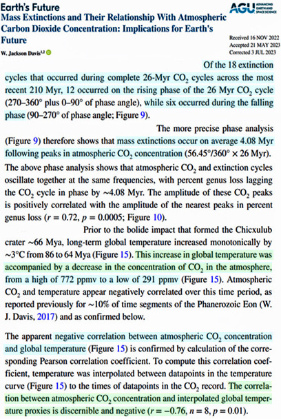
[M]ass extinctions occur on average 4.08 Myr following peaks in atmospheric CO2 concentration … These results collectively require rejection of the hypothesis that long-term (Myr timescale) global temperature change caused extinction of biodiversity across the most highly resolved portion of the fossil record, the last 210 Myr. Prior to the bolide impact that formed the Chicxulub crater ∼66 Mya, long-term global temperature increased monotonically by ∼3°C from 86 to 64 Mya (Figure 15). This increase in global temperature was accompanied by a decrease in the concentration of CO2 in the atmosphere, from a high of 772 ppmv to a low of 291 ppmv (Figure 15). Atmospheric CO2 and temperature appear negatively correlated over this time period, as reported previously for ∼10% of time segments of the Phanerozoic Eon (W. J. Davis, 2017) and as confirmed below. The apparent negative correlation between atmospheric CO2 concentration and global temperature (Figure 15) is confirmed by calculation of the corresponding Pearson correlation coefficient. To compute this correlation coefficient, temperature was interpolated between datapoints in the temperature curve (Figure 15) to the times of datapoints in the CO2 record. The correlation between atmospheric CO2 concentration and interpolated global temperature proxies is discernible and negative (r = −0.76, n = 8, p = 0.01).
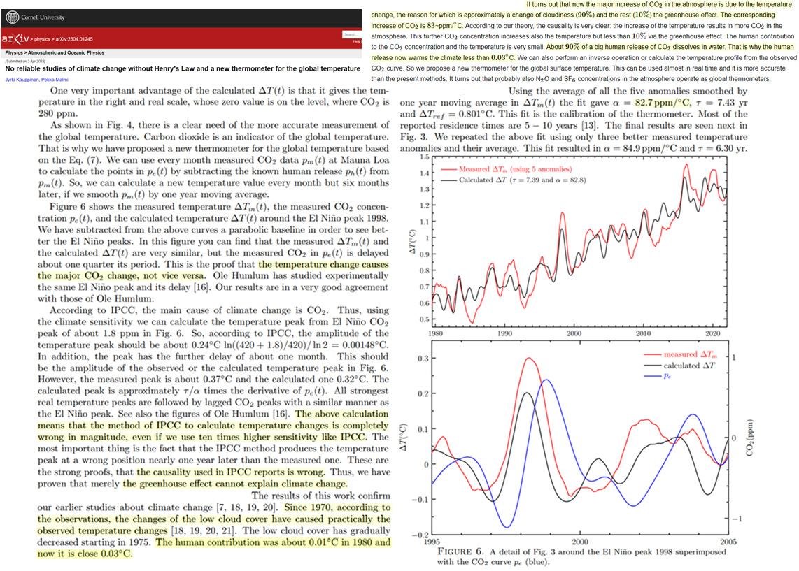
Since 1970, according to the observations, the changes of the low cloud cover have caused practically the observed temperature changes [18, 19, 20, 21]. The low cloud cover has gradually decreased starting in 1975. The human contribution was about 0.01◦C in 1980 and now it is close 0.03◦C.
Koutsoyiannis and Vournas, 2023
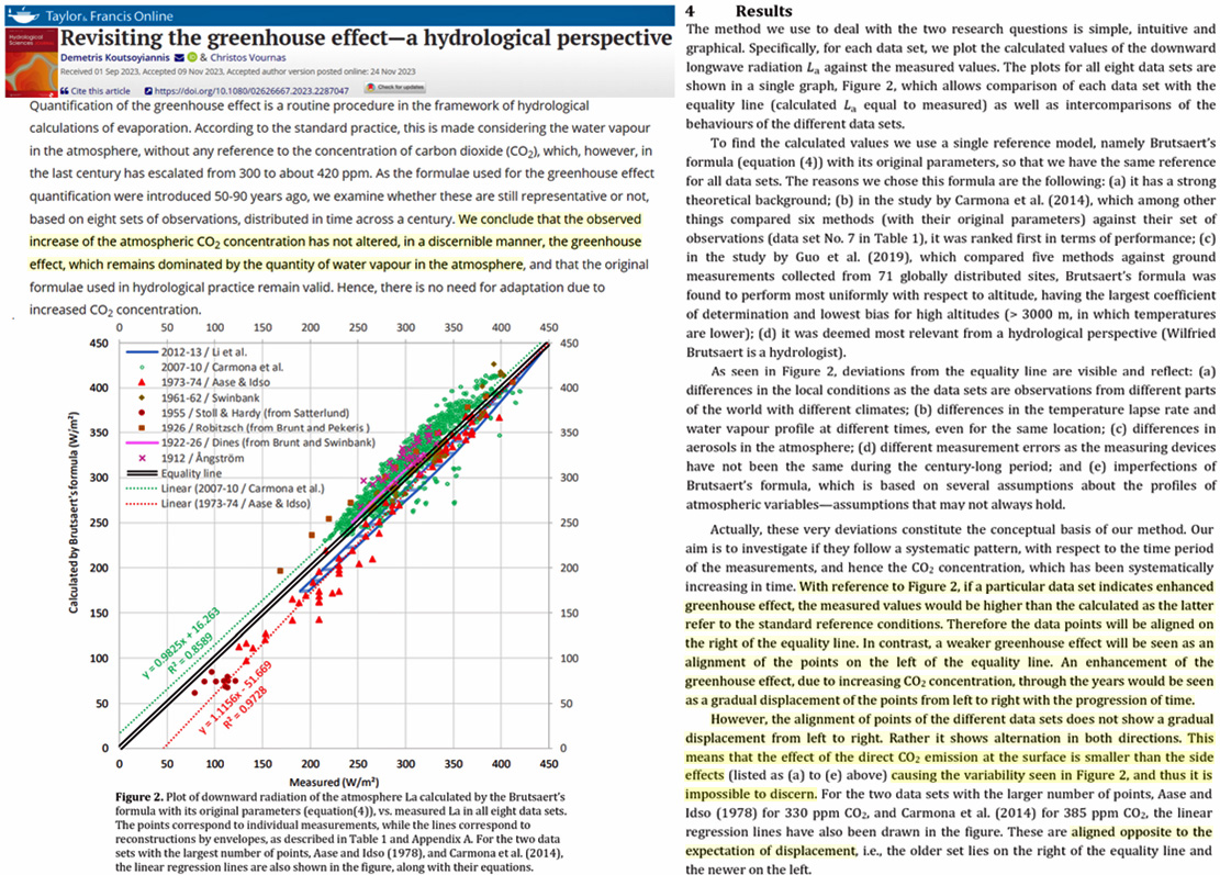
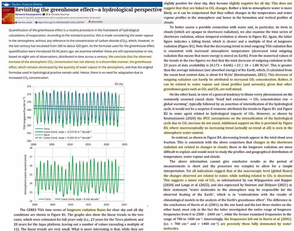
An enhancement of the greenhouse effect, due to increasing CO2 concentration, through the years would be seen as a gradual displacement of the points from left to right with the progression of time. However, the alignment of the points of the different data sets does not show a gradual displacement from left to right. This means that the effect of the direct CO2 emission at the surface is smaller than the side effects…causing the variability in Figure 2, and thus it is impossible to discern. … Quantification of the greenhouse effect is a routine procedure in the framework of hydrological calculations of evaporation. According to the standard practice, this is made considering the water vapour in the atmosphere, without any reference to the concentration of carbon dioxide (CO2), which, however, in the last century has escalated from 300 to about 420 ppm. As the formulae used for the greenhouse effect quantification were introduced 50-90 years ago, we examine whether these are still representative or not, based on eight sets of observations, distributed in time across a century. We conclude that the observed increase of the atmospheric CO2 concentration has not altered, in a discernible manner, the greenhouse effect, which remains dominated by the quantity of water vapour in the atmosphere, and that the original formulae used in hydrological practice remain valid. Hence, there is no need for adaptation due to increased CO2 concentration.
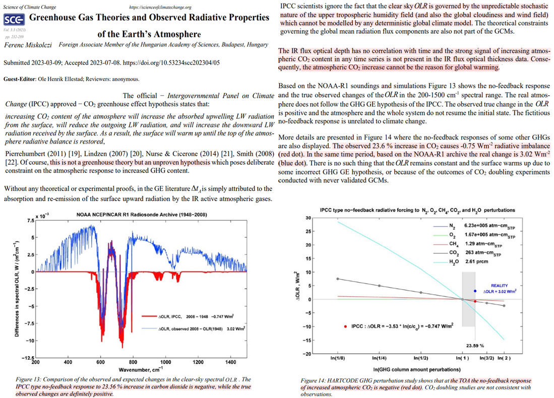
The IR flux optical depth has no correlation with time and the strong signal of increasing atmospheric CO2 content in any time series is not present in the IR flux optical thickness data. Consequently, the atmospheric CO2 increase cannot be the reason for global warming. … The real atmosphere does not follow the GHG GE hypothesis of the IPCC. … More details are presented in Figure 14 where the no-feedback responses of some other GHGs are also displayed. The observed 23.6 % increase in CO2 causes -0.75 Wm-2 radiative imbalance (red dot). In the same time period, based on the NOAA-R1 archive the real change is 3.02 Wm-2 (blue dot). There is no such thing that the OLR remains constant and the surface warms up due to some incorrect GHG GE hypothesis, or because of the outcomes of CO2 doubling experiments conducted with never validated GCMs. … IPCC scientists ignore the fact that the clear sky OLR is governed by the unpredictable stochastic nature of the upper tropospheric humidity field (and also the global cloudiness and wind field) which cannot be modelled by any deterministic global climate model. The theoretical constraints governing the global mean radiation flux components are also not part of the GCMs. … The Arrhenius type greenhouse effect of the CO2 and other non-condensing GHGs is an incorrect hypothesis and the CO2 greenhouse effect based global warming hypothesis is also an artifact without any theoretical or empirical footing. … [T]he atmospheric CO2 increase cannot be the reason for global warming.
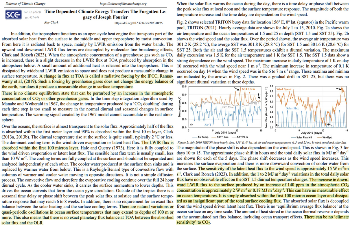
The increase in downward LWIR flux to the surface produced by an increase of 140 ppm in the atmospheric CO2 concentration is approximately 2 W m-2 or 0.17 MJ m-2 day-1. This can have no measurable effect on ocean temperatures. It is simply absorbed within the first 100 micron ocean layer and dissipated as an insignificant part of the total surface cooling flux. The absorbed solar flux is decoupled from the wind speed driven latent heat flux. There is no ‘equilibrium average flux balance’ at the ocean surface on any time scale. The amount of heat stored in the ocean thermal reservoir depends on the accumulated net flux balance, including ocean transport effects. … There can be no ‘climate sensitivity’ to CO2. … There can be no climate equilibrium state that can be perturbed by an increase in the atmospheric concentration of CO2 … CO2 can have no measurable effect on ocean temperatures.
[Transmissivity ] in the CO2 band center is unchanged by increased CO2 as the absorption is already saturated…[T]he water vapor and CO2 overlapping at an absorbing band prevents absorption by additional CO2. … The [doubled CO2] forcing in polar regions is strongly hemispheric asymmetric and is negative in the Antarctic. … The water vapor usually damps the [doubled CO2] forcing by reducing the energy additional CO2 can absorb.
![]()
Unsettled Science, Failed Climate Modeling
The idea that the AMOC will weaken due to climate change has a long history also. Since the mid-1980s, the earliest climate models first predicted that an AMOC slowdown would result from an increase in atmospheric CO2 [7,8]. This projection has been repeated in successive IPCC reports in the intervening 40 years. A large AMOC slowdown is projected to bring a cooler, stormier climate, drier summers and wetter winters, to millions of people, especially in Europe [9,10]. In the most extreme scenario of a complete AMOC collapse where no heat is delivered by the ocean to the northern North Atlantic, a cascade of climate impacts could ensue, accelerating ice loss in West Antarctica, Amazon dieback, and a collapse of arable farming in northwest Europe [11,12]. … Strictly speaking, there is not a single point in time for which a direct measurement of the full AMOC exists. … [W]e find that neither the CMIP5 nor the CMIP6 ensemble mean are successful at representing the observational AMOC data. … We show that both the magnitude of the trend in the AMOC over different time periods and often even the sign of the trend differs between observations and climate model ensemble mean, with the magnitude of the trend difference becoming even greater when looking at the CMIP6 ensemble compared to CMIP5. … [I]f it is not possible to reconcile climate models and observations of the AMOC in the historical period, then we believe the statements about future confidence about AMOC evolution should be revised. … [I]f these models cannot reproduce past variations, why should we be so confident about their ability to predict the future?
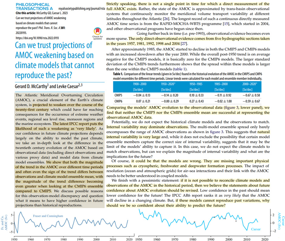
Global climate models (GCMs) from the sixth Coupled Model Intercomparison Project Phases (CMIP6) have been employed to simulate the twenty-first-century temperatures for the risk assessment of future climate change. However, their transient climate response (TCR) ranges from 1.2 to 2.8 °C, whereas their equilibrium climate sensitivity (ECS) ranges from 1.8 to 5.7 °C, leading to large variations in the climatic impact of an anthropogenic increase in atmospheric CO2 levels. Moreover, there is growing evidence that many GCMs are running “too hot” and are hence unreliable for directing policies for future climate changes. Here, I rank 41 CMIP6 GCMs according to how successfully they hindcast the global surface warming between 1980 and 2021 using both their published ECS and TCR estimates. The sub-ensemble of GCMs with the best performance appears to be composed of the models with ECS ranging between 1.8 and 3.0 °C (which confirms previous studies) and TCR ranging between 1.2 and 1.8 °C. This GCM sub-ensemble is made up of a total of 17 models. Depending on the emission scenarios, these GCMs predict a 2045–2055 warming of 1.5–2.5 °C compared to the pre-industrial era (1850–1900). As a result, the global aggregated impact and risk estimates seem to be moderate, which implies that any negative effects of future climate change may be adequately addressed by adaptation programs. However, there are also doubts regarding the actual magnitude of global warming, which might be exaggerated because of urban heat contamination and other local non-climatic biases. A final section is dedicated to highlighting the divergences observed between the global surface temperature records and a number of alternative temperature reconstructions from lower troposphere satellite measurements, tree-ring-width chronologies, and surface temperature records based on rural stations alone. If the global warming reported by the climate records is overestimated, the real ECS and TCR may be significantly lower than what is produced by the CMIP6 GCMs, as some independent studies have already suggested, which would invalidate all of the CMIP6 GCMs. … the trend was 0.03 °C/decade for HadCRUT3, and became 0.08 °C/decade for HadCRUT4 [51], 0.10 °C/decade for HadCRUT5 non-infilled data, and 0.14 °C/decade for HadCRUT5 infilled data
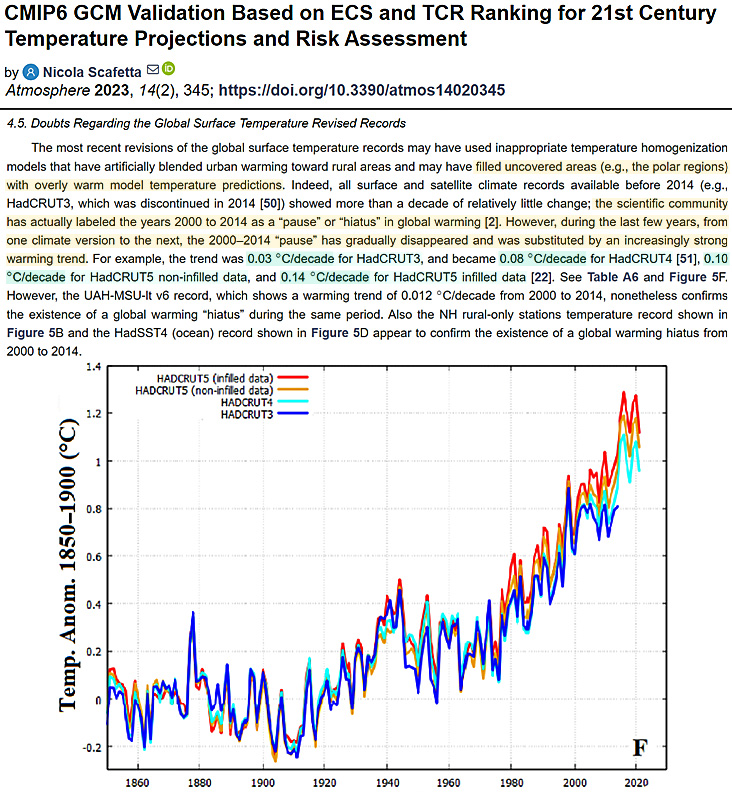
Uncertainty, Error in Calculating Temperature, Climate Forcing Attribution
[A]cross the first 80 years of the 20th century, the analytically basic uncertainty following from the resolution of LiG thermometers alone yields 2σ uncertainty bounds averaging 4× the published 95% confidence interval for the global air-temperature record of 1900, more than 5× after 1950, and 13× by 1980. The uncertainty stemming from the laboratory resolution limit of LiG thermometers alone is sufficient to obscure the rate and magnitude of climate warming since 1900. … The compilation of land- and sea-surface [thermometer] uncertainty yield a 1900-2010 global air-temperature record anomaly of 0.86 ± 1.92°C (2 σ), which renders impossible any conclusion regarding the rate or magnitude of climate warming since 1850 or earlier. … For SSTs, the available bucket and engine-intake field calibrations show that shipboard SST measurement errors are, likewise, not random. The uncertainties attached to bucket SSTs, 2σ = ±0.4°C and engine-intake SSTs 2σ = ±2°C… Each of the engine-intake calibrations yielded a bias and uncertainty of 0.3 ±1.2°C (1σ), which obviates accuracy. … The magnitude of the SST error mean itself remains unknown. … The results indicated that a shipboard bucket seawater sample will not accurately convey the physically true sea-surface temperature unless three conditions are simultaneously true: (1) the thermocline is absent; (2) the vessel is heading into the wind; and (3) the mixing layer extends well below the depth of the keel.
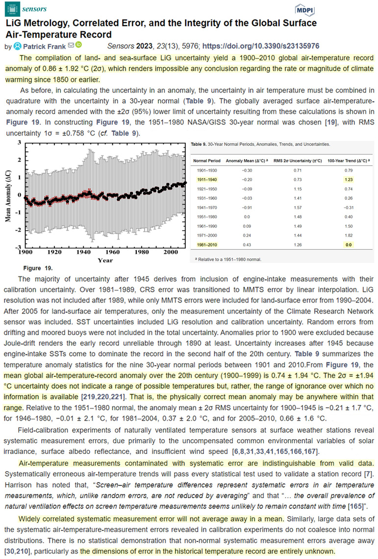
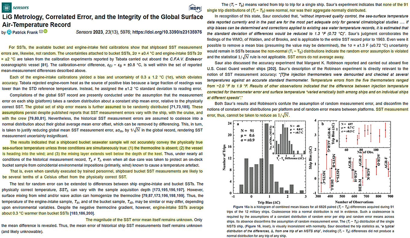
As both drivers and first responders, urban areas are rapidly increasing in importance of shaping global climate change. The global imprint of urbanization on surface energy balance (SEB) remains, however, largely unknown. Here, we undertake a global spatiotemporal analysis on urbanization-induced Earth’s surface energy alteration using annually dynamic maps of impervious surface and satellite-derived surface energy fluxes and land surface temperature (LST), alongside space-for-time (spatial) and time for-time (temporal) approaches. Relying on spacefor-time substitution, we estimate that global urbanization-driven surface warming of annual mean temperature has reached 0.054 ◦C (95% CI, − 0.009–0.214 ◦C) between 2003 and 2018 (with temporal stability), especially pronounced in summer daytime (0.122 ◦C, − 0.038–0.495 ◦C), largely attributed to decline in local latent heat cooling, enlarged long-wave heat dissipation and anthropogenic heat.
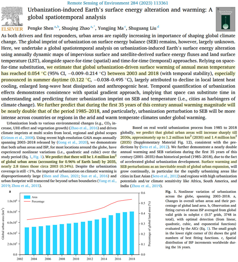
There is now compelling evidence that the lack of resolution of coarse global models and even coarsely resolved mesoscale cloud models and the inability to explicitly resolve convection specifically is a major obstacle in making the advances needed to confront important Earth science challenges of today (Slingo et al. 2022). The inset example of Fig. SB2, taken from the global model study of Miyamoto et al. (2013), offers a clear example of the influence of model resolution on the properties of convection and why models are pushing further and further into the domain of the “terra incognita.” … Existing climate models…cannot resolve the detailed structure and life cycles of systems such as tropical cyclones, depressions, and persistent high pressure systems, which are key in the coupling of the energy and water cycle. … [P]resent day global models are also unable to resolve ocean currents that are fundamental to climate variability. … [N]one of the techniques available today enable us to estimate the EEI with the perceived required accuracy less than ±0.3 W/m², let alone with an aspirational accuracy of ±0.1 W/m².
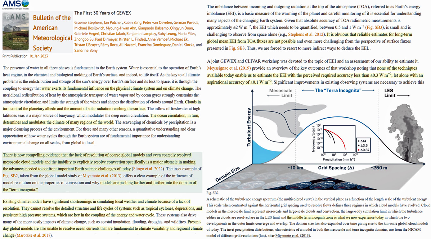
Aerosols, such as airborne wildfire smoke, desert dust, volcanic and pollution particles, affect Earth’s climate by reflecting (some also absorb) sunlight. These aerosol particles also play key roles in cloud formation and evolution, further affecting the planet’s energy balance. The magnitudes of these effects, and even the underlying mechanisms, represent the largest uncertainty in climate modeling. Despite two decades of advances in many aspects of aerosol-climate science, aerosol climate forcing uncertainty is virtually undiminished. Yet, reducing this uncertainty is critical for any effort to attribute, mitigate, or predict climate changes. … A lower bound on the uncertainty range of just the direct component of the total global-mean all-sky aerosol forcing (i.e., that due to scattering and absorption by airborne particles but not their indirect effects on clouds) is estimated as ±1.1 W/m2 when considering anticipated data from a planned next-generation NASA satellite mission aimed at addressing global climate change issues(1; Thorsen et al., 2021). … Model representation of aerosol properties often fails to capture the complexity found in nature, particularly in bulk models lacking microphysics, and generally, differences among commonly used aerosol representations in models can produce very different aerosol forcing results in model simulations (Nazarenkpo et al., 2017). … Many of the relevant processes operate on spatial scales far smaller than the resolution of global models and are therefore either highly parameterized or simply not included, such as some aerosol effects on convective clouds. Large Eddy Simulations (LES) are valuable research tools, complementary to climate models in that they can resolve many of the smaller-scale processes; however, they still entail assumptions that are often unconstrained by measurements, are impractical to run over large areas or long time periods, and cannot provide estimates of forcing (e.g., Bellouin et al., 2020). … In summary, many of the factors that dominate aerosol-cloud-radiation interactions, such as CCN concentration and composition, are difficult to measure with space-based remote sensing; this is especially true for efforts to obtain coincident aerosol and related cloud properties. As such, knowledge of these quantities remains limited on a global scale (e.g., Seinfeld et al., 2016), leaving model-simulated aerosol indirect effects inadequately constrained by observations. Except in special circumstances and with stringent assumptions (e.g., Pahlow et al., 2006; Rosenfeld et al., 2016; Dawson et al., 2020), quantitative constraints on nearly all the key variables needed to characterize detailed ACI are beyond the capabilities of existing and currently planned space-based remote-sensing instruments.
Owing to the complexity of physical processes in the atmosphere and hydrosphere, several numerical climate models possess uncertainties that exceed certain relevant, either observed or predicted, effects of global warming by orders of magnitude. Lauritzen et al. ([2] p. 2) found that some “models that conserve energy and water mass do not match an observed global mean precipitation rate. … The energy balance still suffers from significant errors. The causes of these errors are largely unknown, but are observed to be large over tropical oceans. … [In] pre-industrial simulations from a wide range of IPCC climate models, … most climate models featured biases of the order of 1 W m −2 for the net global and the net atmospheric, oceanic, and land energy balances. … These imbalances are partly due to imperfect closure of the energy cycle in the fluid components.” To demonstrate the significance of that uncertainty, a minor heating flux of just 0.005 W m−2 is sufficient to raise the atmospheric temperature at an observed rate of 2 °C per century [3,4,5,6,7]. “The oceans have a heat capacity about 1000 times greater than the atmosphere and land surface” ([8] p. 420). If also expressed per global surface unit area, even an increase in the large oceanic heat content by as much as 0.5 W m −2 ([8] p. 427), [9,10] would remain well below the model uncertainty range. However, “the climate of the Earth is ultimately determined by the temperatures of the oceans” ([8] p. 420).
The accuracy of cloudy-sky radiation estimates strongly depends on how accurately the cloud properties are simulated. Unfortunately, even reanalysis products are prone to radiative biases in the Southern Ocean (Trenberth and Fasullo 2010), likely also due to the sparse data of cloud properties. Recently, shortwave radiation errors of up to 39 W m−2 in the Modern-Era Retrospective Analysis for Research and Applications, version 2 (MERRA-2), were found using ship-based observations in the Southern Ocean during austral summer (Kuma et al. 2020). Similarly, daily errors of 60 W m−2 in the fifth major global reanalysis produced by the European Centre for Medium-Range Weather Forecasts (ERA5) have also been reported in the Southern Ocean and associated with biases in cloud fraction and transmittance (Wang et al. 2020). … … Earth system models struggle to simulate clouds and their radiative effects over the Southern Ocean, partly due to a lack of measurements and targeted cloud microphysics knowledge. We have evaluated biases of downwelling shortwave radiation in the ERA5 climate reanalysis using 25 years (1995–2019) of summertime surface measurements, collected on the Research and Supply Vessel (RSV) Aurora Australis, the Research Vessel (R/V) Investigator, and at Macquarie Island. During October–March daylight hours, the ERA5 simulation of SWdown exhibited large errors (mean bias = 54 W m−2, mean absolute error = 82 W m−2, root-mean-square error = 132 W m−2, and R2 = 0.71).
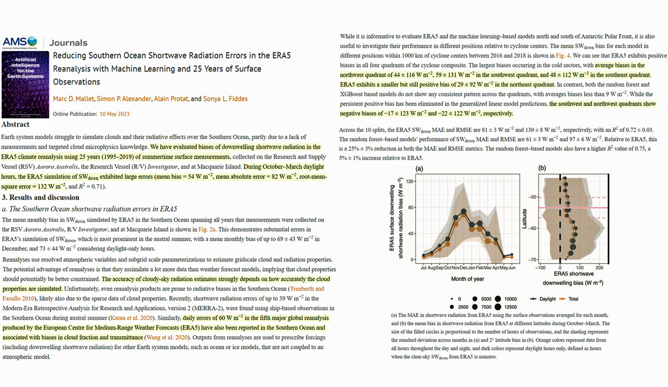
Weather and climate phenomena have outsized impacts on society when they are particularly extreme. Extreme Event Attribution (EEA) seeks to quantify the extent to which extreme weather and climate phenomena are the result of anthropogenic climate change (ACC), and thus it has implications for many pertinent climate change discussions, including those on potential legal claims of loss and damages and calculations of the social cost of carbon. The Fraction of Attributable Risk (FAR) is one metric that is used to quantify the proportion of an extreme weather or climate “event” associated with ACC. The FAR is typically applied to changes in the likelihood of exceeding some geophysical value chosen, post hoc, to represent the “event” (e.g., i.e., rainfall amounts, flood depths, drought measures, temperature values, etc.). The FAR has further been used to estimate the fraction of observed impacts (e.g., lives lost or economic damage) that can be associated with ACC by multiplying realized impacts by the FAR (IFAR = Impact×FAR). Here, we illustrate with a few stylized examples that this IFAR calculation only produces reliably useful results when the weather or climate phenomena in question can be easily conceived of as a discrete binary “event” (i.e., the entirety of the event either occurs or it does not). We show that the IFAR calculation can produce misleading results when the weather or climate phenomena in question are on a continuum, and ACC can be thought of as altering the intensity of the geophysical value that is used in the eventhood definition. Specifically, we show that the IFAR calculation inflates the impacts associated with ACC in these circumstances because it inaccurately assumes that there would have been zero impact had the geophysical value chosen to define eventhood not been exceeded. We illustrate that for weather and climate phenomena on a continuum (e.g., floods, droughts, temperatures, etc.), a clearer way of conceptualizing the impacts associated with ACC is to compare the expected value of the impact between the ACC and preindustrial conditions across the full continuum.
Failing Renewable Energy, Climate Policies
The central estimate of the costs of climate policy, unrealistically assuming least-cost implementation, is 3.8–5.6% of GDP in 2100. The central estimate of the benefits of climate policy, unrealistically assuming high no-policy emissions and constant vulnerability, is 2.8–3.2% of GDP. … The central estimate is that the costs exceed the benefits throughout the 21st century … In 2050, the year of net-zero, the best estimate of the benefits of the 1.5∘C target are about 0.5% of GDP while the costs are almost 5%. … Riahi et al. (2022) reports that the global average carbon tax needed to meet the 1.5∘C temperature target ranges between $30/tCO2 and $1,100/tCO2 in 2030 and between $110/tCO2 and $14,000/tCO2 in 2100. That target would cost somewhere between 0.5% and 6.0% of GDP in 2030, and up to 10% in 2100. … The central estimate of the benefits is always smaller than the central estimate of the costs. Ignoring the uncertainty for the moment, regardless of the discount rate, the present costs exceed the present benefits; the net present benefits are negative.
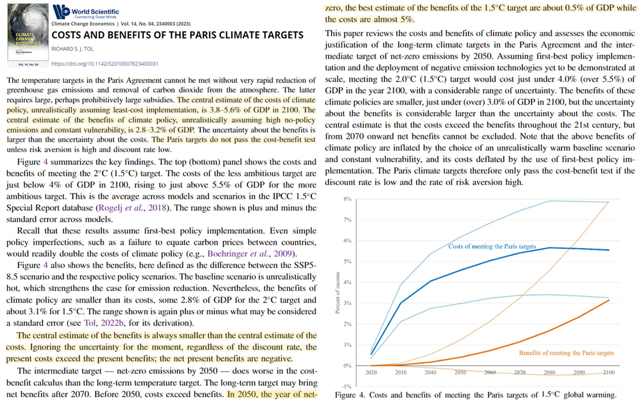
In order to realistically fulfil global and national climate protection targets, all potential measures have to be made use of to a maximum extent. Because it is readily available, biomass energy has been playing a key practical role for decades, supported by the traditional assumption of its carbon neutrality: under sustainable conditions, carbon dioxide emitted during combustion is held to be equal to its absorption during plant growth. In order to clarify conditions of carbon (C) neutrality, it is therefore necessary to model the annual natural C cycle on the entire planet and to include changes caused by a variety of growth strategies for biomass fuels. The “Combined Energy and Biosphere Model” CEBM calculates the cycle of plant growth, decay, biomass fuel production and its combustion on 2433 grid elements worldwide. CEBM results suggest that over many decades, the C pools of litter and especially soil organic carbon (i.e., humus layer) deplete considerably as a consequence of the interrupted natural carbon cycle. Overall, based on this finding, the earlier assumption of “carbon-neutral biomass fuels” is disapproved of in a long-term evaluation and—as a coarse rule of thumb—might be reduced to “half as carbon neutral as previously assumed” (when compared to a current fuel mix). On top of this principal effect, it is well known that life-cycle emissions, indirect or secondary emissions such as energy input related to production, transport and conversion into fuels will still add to this already principally highly incomplete carbon neutrality of biomass.
Impacts of wind power on bats are usually evidenced by the recorded fatalities, while other impacts are not well understood or considered during project planning. However, wind turbines may affect use of the surrounding habitats by bats. Little is known about such impact, especially in the European boreal biogeographical region. We studied the consequences of operating wind turbines on the presence and activity of bats in forests. We simultaneously monitored bat acoustic activity at 84 sampling sites placed at 200 m intervals from 0 to 1.000 m (2 recorders per distance class), over four months and at seven Finnish wind farms located in forested habitats. Our results show higher presence and activity at 600 m and further from turbines for Eptesicus nilssonii, and higher presence at 800 m and further for Myotis spp. We also saw an increase in bat activity during midsummer, which may be due to increased use of forest canopy cover during the short nights at this time. These results indicate a potential loss in habitat quality around wind turbines, e.g., a greater number of open areas in forests unfavourable to certain bat species. This lower activity and presence could also be an indication for active avoidance of the wind turbines from the bats. Furthermore, these results are the first of their kind for Eptesicus nilssonii, and for the European boreal biogeographical region. They show undeniable impacts of wind power on bats in Finland, and enforce the requirement for better consideration of bats during the development of such projects in Finland. Similarly, these results show impacts of operating turbines on habitat use by bats, impacts that now must be considered in Europe. We also call for investigation on the causative mechanisms of the observed effect, to better facilitate mitigation.
Testing and documenting effects of wind farm (WF) infrastructure on wildlife are crucial considering increasing development throughout Scandinavia, especially for reindeer, which require large areas for grazing and are vulnerable to disturbances. We present results from 2011 to 2019 for semidomesticated reindeer tracked with Global Positioning System (GPS) transmitters, along with herders’ knowledge about reindeers’ habitat use and changes following WF development within the Raggonjarga reindeer district summer range in Finnmark, Norway. We tracked up to 36 females (ranging from 19 to 36 individuals per year), from their arrival in the study area in April to their departure in the end of October. We evaluated habitat use before, during, and after WF development at the home range and landscape scales. We also evaluated reindeer habitat use qualitatively based on semistructured interviews with local herders. The herders’ reported negative effects of the WF on reindeer, both on general habitat use and intrarange movements, resulting in less use of grazing areas surrounding the WF and increased workload for the herders.
Corals Thrive In Warm, High CO2 Environments
…average cover of corals in October, 2020, six months after the bleaching, did not differ from that initially recorded in April 2020 at both shallow and deep sites
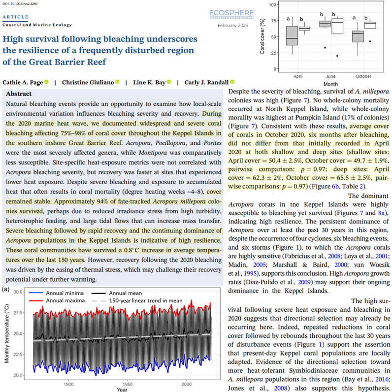
The annual growth rates of these coral colonies ranged from 0.65 cm/yr to 1.77 cm/yr (Fig. 2A). The two most recent cores have an average growth rate of 1.23 ± 0.22 cm/yr in the 20th century, which is similar to two previously reported Xisha Porites corals (1.16 ± 0.37 cm/yr and 1.10 ± 0.22 cm/yr, Table 1) for the same period (Kang et al., 2021; Yan et al., 2019). The average growth rate of four colonies living in the LIA is 0.87 ± 0.11 cm/yr, which is significantly (t-test, p < 0.0001) lower than the colonies in the 20th century. … The observed low average growth rates during the LIA can be explained by the ~1°C lower temperature … [A]nthropogenic CO2 can only induce a ~0.1 pH unit drop in pHsw, which translates into about 0.05 units of pHcf variation
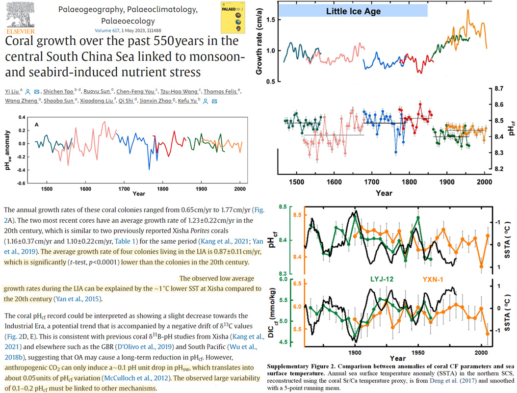
This study compared corals adapted to variable pHT (i.e., 7.23–8.06) from the semi-enclosed lagoon of Bouraké, New Caledonia, to corals adapted to more stable seawater pHT (i.e., 7.90–8.18). In a 100-day aquarium experiment, we examined the physiological response and genetic diversity of Symbiodiniaceae from three coral species (Acropora tenuis, Montipora digitata, and Porites sp.) from both sites under three stable pHNBS conditions (8.11, 7.76, 7.54) and one fluctuating pHNBS regime (between 7.56 and 8.07). Bouraké corals consistently exhibited higher growth rates than corals from the stable pH environment. … [L]ong-term exposure to pH fluctuations and/or differences in symbiont communities benefit calcification under OA.
A decline in the rate of sea-level rise, as observed after 6 ka BP, has diminished accommodation space and, hence, reef accretion. Rate of rise in Holocene sea level and reef accretion rate indeed exhibit a positive correlation (Fig. 3B). Likewise, a mid-to-late Holocene temperature fall has been suggested to be responsible for reef decline in Beliz, as well as south Florida. Coral sclerochronology and vegetation data from offshore Belize suggest also that warm and wet conditions during early Holocene times were followed by cooler and drier conditions in the mid-late Holocene. … [D]ata from Florida, the Virgin Islands, and Belize barrier and atoll reefs indicate individually and collectively that significant acroporid declines apparently did occur in the pre-Anthropocene era. The results of the present study suggest that there are gaps in the Holocene A. palmata record, and, that A. cervicornis was twice as abundant during the early as compared to the mid and late Holocene (13.1 ± 1.7% vs. 6.7 ± 1.4% and 6.3 ± 1.7%, respectively), suggesting a deterioration in the environmental conditions for reef development over time
Here, we reveal an emergent increase in the thermal tolerance of coral assemblages at a rate of 0.1 °C/decade for a remote Pacific coral reef system. This led to less severe bleaching impacts than would have been predicted otherwise, indicating adaptation, acclimatisation or shifts in community structure. Using future climate projections, we show that if thermal tolerance continues to rise over the coming century at the most-likely historic rate, substantial reductions in bleaching trajectories are possible.
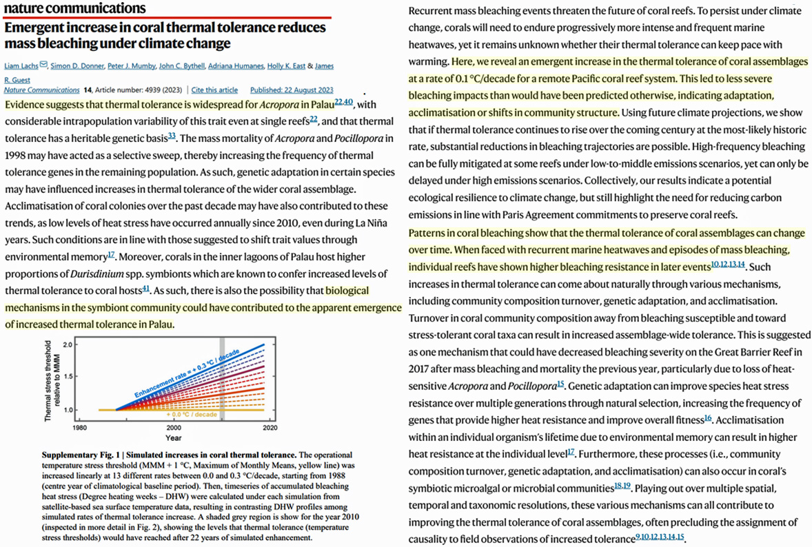
Elevated CO2: Greens Planet, Higher Crop Yields
Higher warming will affect more regions globally with intensified agricultural and ecological droughts. Higher CO2 concentration improves vegetation’s water use efficiency (WUE), but its potential to alleviate extreme agricultural and ecological droughts is unclear. India is the second-highest contributor to global greening, having two of the eight global hottest biodiversity hotspots. Here, for the first time, using the CMIP6 earth system models (ESMs), we found an increase in the net vegetation productivity in India at the rate of 10.552 TgC year−1 with 1% per year increase in atmospheric CO2 concentration from 285 ppm to 1140 ppm, contrary to global trends. The improved WUE resulting from carbon fertilization and higher rain under warming will supersede the increased evapotranspiration water loss due to radiative effects. We found that the substantial increase in vegetation productivity in India attributes to plant physiology, and such factor needs to be considered in the drought projections. … Overall, there is high consistency across the models that India will experience a reduced ecological drought with increased productivity under increased CO2 concentration. We found that the plant can sustain better even in drought scenarios in the future, compared to the present, due to carbon fertilization.
Therefore, the random forest reconstruction results can better reflect changes in regional tree cover, which was approximately 38%–42% during 2000–200 Cal yr BP. It then obviously increased from a low value of approximately 40% to a modern level of approximately 45%. The precipitation and carbon dioxide (CO2) concentration were the main drivers for the tree cover before and after 200 Cal yr BP, respectively. This indicates that environments with elevated CO2 level in the near future will benefit the growth of vegetation in the central–northern parts of the Daxing’an Mountains.
Globally, eCO2 [elevated CO2] significantly increased photosynthetic rate (Pn) and instantaneous water use efficiency (WUEi) by 40.8% and 62.1%, respectively, which also had positive effects on forage dry matter yield (DMY) (+25.1%), especially for forage in Northern Europe.
According to satellite observations, the earth has been experiencing widespread vegetation greening since the 1980s, primarily due to large-scale climate change and CO2 fertilization effects. Such greening could mitigate global warming by triggering negative biochemical feedback to the climate system, which refers to increasing CO2 removal from the atmosphere through the vegetation photosynthesis process.
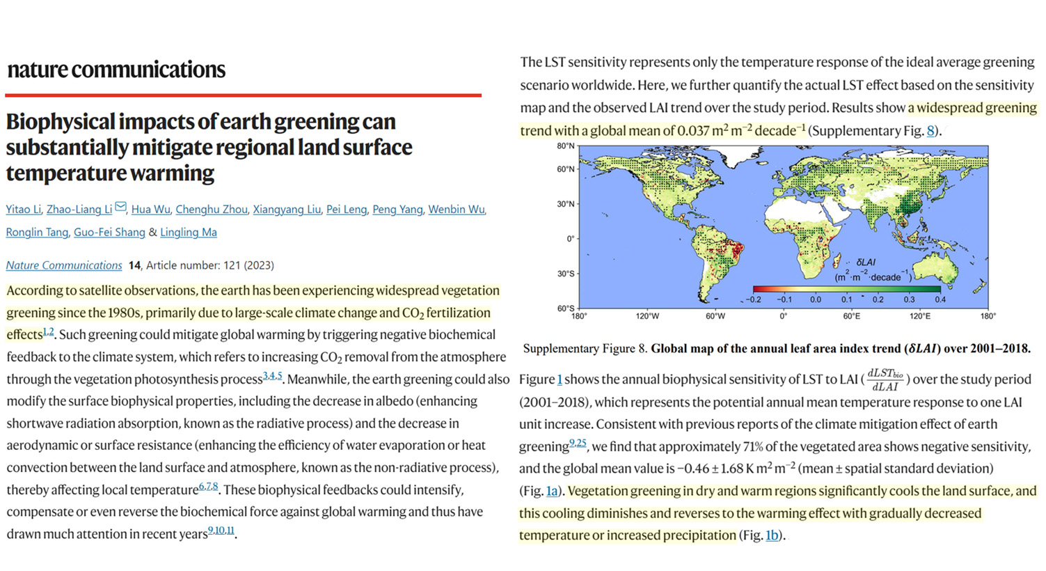
Global dryland areas are vulnerable to climate change and anthropogenic activities, making it essential to understand the primary drivers and quantify their effects on vegetation growth. In this study, we used the Time Series Segmented Residual Trends (TSS RESTREND) method to attribute changes in vegetation to CO2, land use, climate change, and climate variability in Chinese and American dryland areas. Our analysis showed that both Chinese and American drylands have undergone a greening trend over the past four decades, with Chinese greening likely linked to climatic warming and humidification of Northwest China. Climate change was the dominant factor driving vegetation change in China, accounting for 48.3%, while CO2 fertilization was the dominant factor in American drylands, accounting for 47.9%. However, land use was the primary factor resulting in desertification in both regions. Regional analysis revealed the importance of understanding the drivers of vegetation change and land degradation in Chinese and American drylands to prevent desertification. These findings highlight the need for sustainable management practices that consider the complex interplay of climate change, land use, and vegetation growth in dryland areas.
Massive Natural CO2 Fluxes
CO2 volcanic vent near Panarea Island (Italy). This underwater crater at 10 m releases persistent gaseous emissions (98-99% CO2)
New research finds that ancient carbon in rocks releases as much carbon dioxide as the world’s volcanoes … New research has overturned the traditional view that natural rock weathering acts as a CO2 sink that removes CO2 from the atmosphere. Instead, this can also act as a large CO2 source, rivalling that of volcanoes. The results have important implications for modelling climate change scenarios but at the moment, CO2 release from rock weathering is not captured in climate modelling. … However, for the first time this new study measured an additional natural process of CO2 release from rocks to the atmosphere, finding that it is as significant as the CO2 released from volcanoes around the world. Currently, this process is not included in most models of the natural carbon cycle.
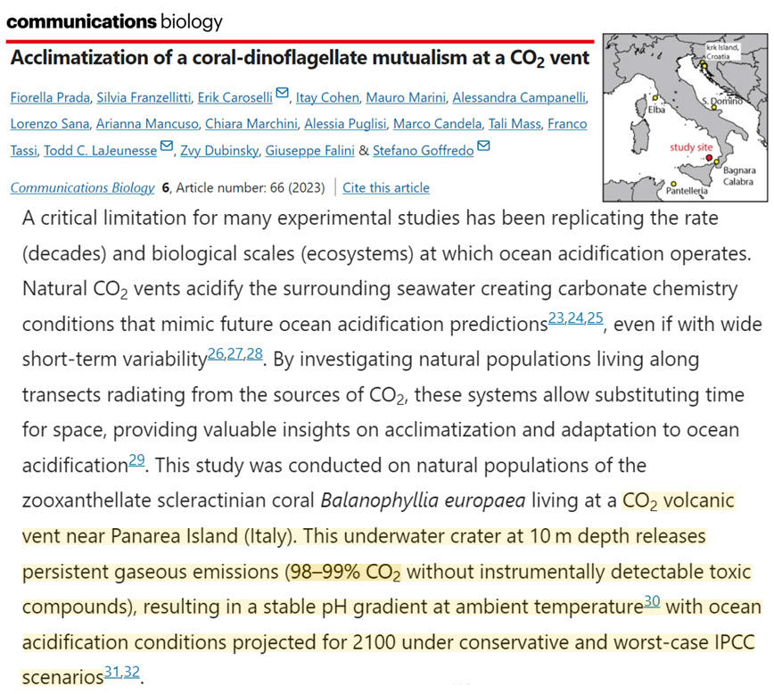
We find a CO2 release of 68+18−6 megatons of carbon annually from weathering of OCpetro in near-surface rocks, rivalling or even exceeding the CO2 drawdown by silicate weathering at the global scale … Within uncertainties, rock weathering in about a third of the major river basins is a net source of CO2 after OCpetro oxidation is considered, even while using the values of initial atmospheric CO2 consumption of silicate weathering rather than the smaller quantity of CO2 eventually locked up in the lithosphere through carbonate precipitation of the associated released dissolved ions (Fig. 2a). The Yangtze (Changjiang) and Mekong draining the eastern flanks of the Himalayas and the Mackenzie River draining shales west of the Rockies in Canada are major sources of CO2 from rock weathering. These high-emitting basins have in common some of the highest basin-average denudation rates and OCpetro stocks (Fig. 2b,c), which is consistent with OCpetro oxidation being driven by OCpetro stocks and denudation (equation (1))7,8,25.
The knowledge of the global distribution of seamounts is still incomplete because only 20% of the seafloor has been mapped by ships (Mayer et al., 2018) … We used the latest grid of VGG to update and refine the global seamount catalog; we identified 19,325 new seamounts, expanding a previously published catalog having 24,643 seamounts.
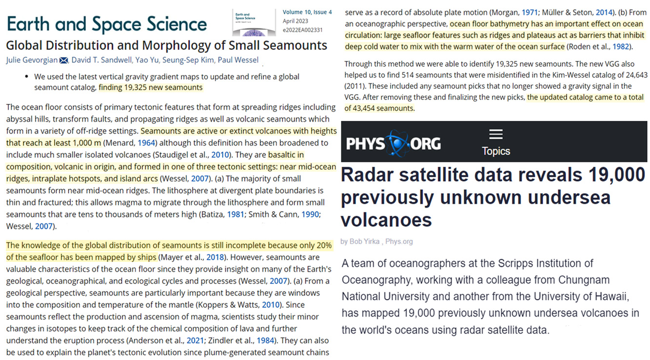
Adding Water Vapor (Via Irrigation) – Earth’s Main GHG – Cools the Surface Atmosphere
Our results show that irrigation could potentially reduce the mean seasonal maximum temperature during the Angry summer of 2012/2013 by −1.44°C to −2.13°C over irrigated regions.
We found the space-and-time method can better represent the cooling effects of long-term irrigation expansion than the space-for-time method, despite that they derived similar cooling trends. The cooling effects were most evident in South Xinjiang, followed by North Xinjiang and Hexi Corridor, and varied in different irrigation expansion sources. Specifically, more intensive cooling occurred in new irrigated areas from unused lands (-0.69 ± 0.02 K) than that from grasslands (-0.47 ± 0.05 K) and forests (-0.28 ± 0.04 K). The cooling effects were dominated by marked daytime cooling compared to negligible nighttime warming.
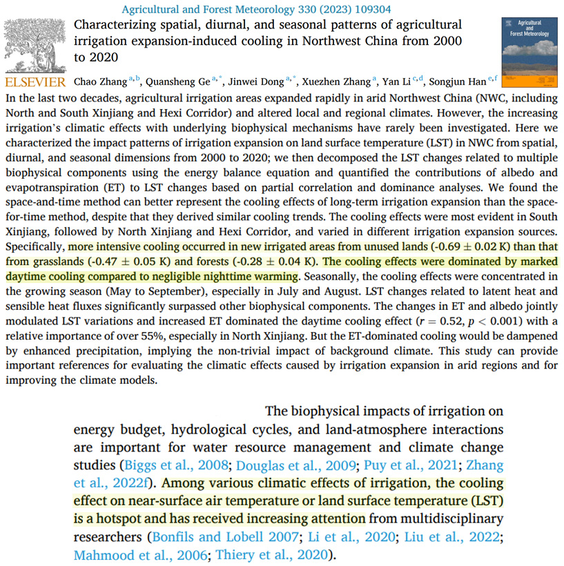
Miscellaneous
Measurements from the Copernicus Sentinel-5P satellite show that this year’s ozone hole over Antarctica is one of the biggest on record. The hole, which is what scientists call an “ozone depleting area,” reached a size of 26 million sq km on 16 September 2023. This is roughly three times the size of Brazil.
The pragmatic prognosis is that we must reduce the emission of greenhouse gases to zero if global temperature is to be stabilized, and such a radical goal “means that the shape and structure of modern capitalism will have to be changed” as the fossil-fuel sector underpins much of our present-day economy. … The foremost tool for shifting the economy to address climate change is the introduction of carbon pricing (whether in the form of a tax or tradeable permit) to create market signals that will steer corporate strategy and entrepreneurial activity towards less carbon intensive activities. While important as one tool for dealing with this issue, it will not be enough to bring about the full-scale systems change that brings carbon emissions to zero on the time scale that is needed. … If we don’t come to terms with climate change by 2030, damage to the global climate will be irreversible. … A future in which we address climate change may require that the entire sector be euthanized, imposing death ahead of its imminent arrival. … An important step in any triage operation is coming to terms with the extreme decision that has to be made for the patient, the doctor and those affected by the decision. Today, there are signs that many within the fossil-fuel sector are not ready to face the prognosis that faced the tobacco industry.
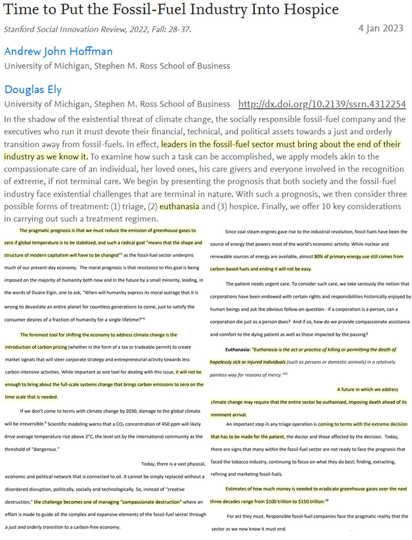
We studied the interactive impacts of copper (Cu) and CO2 enrichment on two natural phytoplankton communities from the eastern and central Arabian Sea. … Interestingly, CO2 enrichment seemed to alleviate Cu toxicity in some species (Nitzschia sp., Cylindrotheca closterium, Guinardia flaccida, and Phaeocystis) and increased their growth rates. This could be related to the cellular Cu demand and energy budget at elevated CO2 levels.
Exhaled human breath can contain small, elevated concentrations of methane (CH4) and nitrous oxide (N2O), both of which contribute to global warming. These emissions from humans are not well understood and are rarely quantified in global greenhouse gas inventories. … It has been reported that exhaled human breath can contain the greenhouse gases methane (CH4) and nitrous oxide (N2O) [1, 2], both of which have a much higher global warming potential than carbon dioxide (CO2) (34 and 265 for CH4 and N2O, respectively [3]). Where hydrocarbon chains (food types) are consumed by humans and turned into CH4 (and N2O from nitrogen intake), the global warming potential is no longer neutral, and human respiration has a net warming effect on the atmosphere.
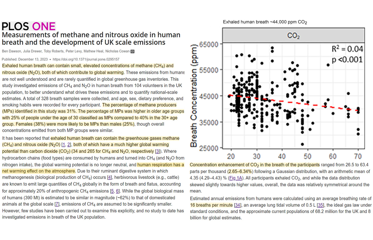
[E]ven after controlling for demographic characteristics, personality characteristics, and environmental attitudes, overall environmental knowledge and climate-specific knowledge were negatively related to climate change anxiety.
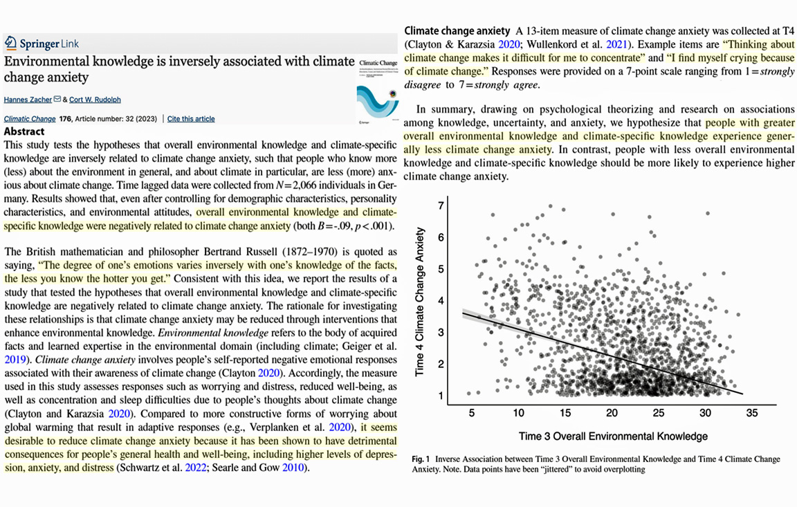
Anthropogenic activity is considered a central driver of current climate change. A recent paper, studying the consensus regarding the hypothesis that the recent increase in global temperature is predominantly human-made via the emission of greenhouse gasses (see text for reference), argued that the scientific consensus in the peer-reviewed scientific literature pertaining to this hypothesis exceeds 99%. This conclusion was reached after the authors scanned the abstracts and titles of some 3000 papers and mapped them according to their (abstract) statements regarding the above hypothesis. Here, we point out some major flaws in the methodology, analysis, and conclusions of the study. Using the data provided in the study, we show that the 99% consensus, as defined by the authors, is actually an upper limit evaluation because of the large number of “neutral” papers which were counted as pro-consensus in the paper and probably does not reflect the true situation. We further analyze these results by evaluating how so-called “skeptic” papers fit the consensus and find that biases in the literature, which were not accounted for in the aforementioned study, may place the consensus on the low side. Finally, we show that the rating method used in the study suffers from a subjective bias which is reflected in large variations between ratings of the same paper by different raters. All these lead to the conclusion that the conclusions of the study does not follow from the data.
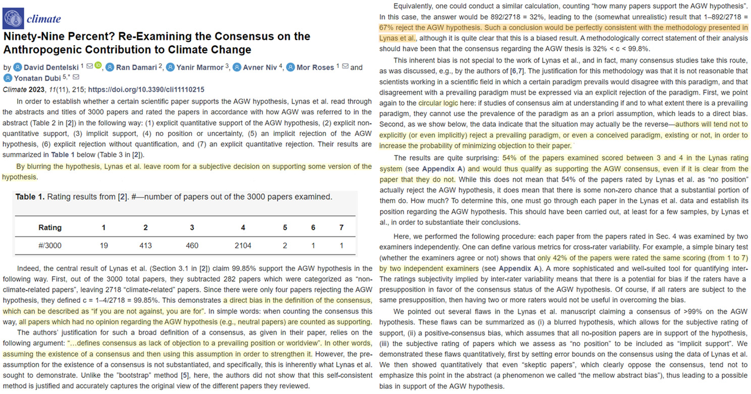
Paleoecological records of past fire events and forest composition provide long-term ecological context for modern changes in fire regimes and forest dynamics. Here, we use pollen and contiguous macroscopic charcoal analyses of lake sediments from Pender Island, British Columbia, Canada to reconstruct changes in fire regimes over the last 10,000 years and investigate how these interact with changes in climate and forest composition with a focus on fire-related plant functional types. The relatively warm and dry early Holocene was characterized by high charcoal accumulation rates, fire episodes of moderate severity, and a mean fire return interval of 100 ± 27 years. Forests at the time were open-canopy Pseudotsuga menziesii forests with abundant fire endurer taxa (e.g., Pteridium aquilinum) that have a competitive advantage in regimes of frequent fire. Fire continued to occur every ~100 years, on average, during the establishment of Quercus garryana savanna communities; however, a decrease in charcoal peak magnitudes suggests the fire regime shifted to one characterized by smaller and/or lower intensity surface fires. As temperature and moisture deficits decreased in the mid- and late Holocene (i.e., after ~6000 calendar years before present), mean fire return intervals lengthened to 176 ± 54 years and increased variability in charcoal peak magnitudes suggests a mixed fire regime of low-moderate-intensity fires combined with infrequent crown or stand-replacing fires.
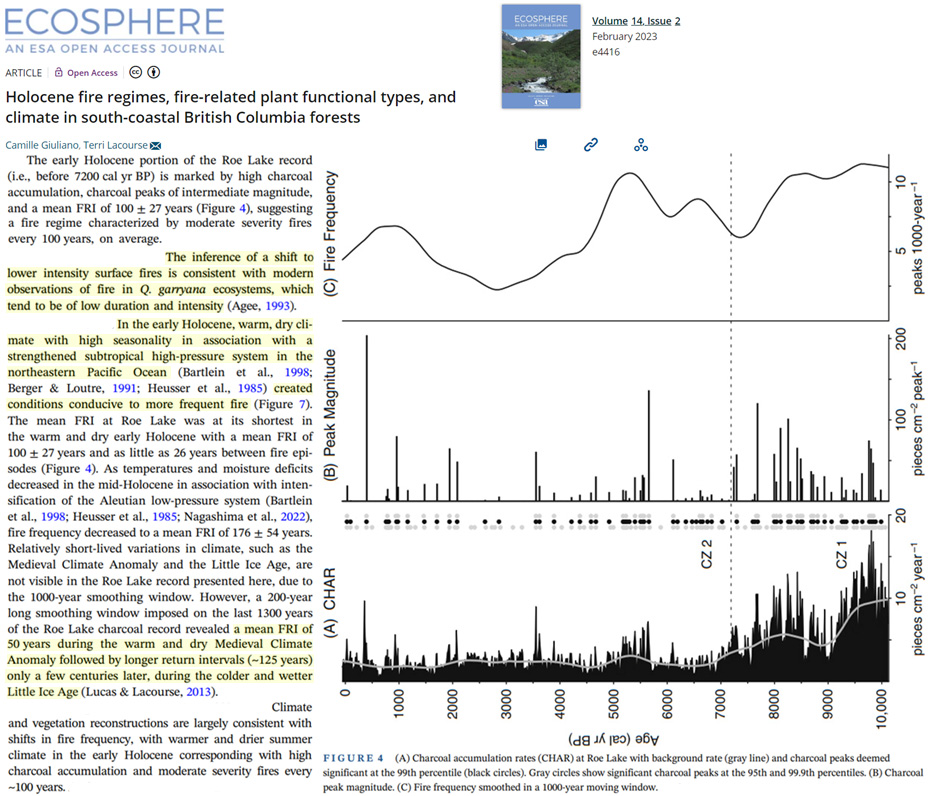
Despite high local elevations of CO2 when wearing surgical facemasks, humans might have become adapted to long-term wear and high CO2 exposure, and cognition was not severely inhibited. … One study by Rhee M et al. determined for a KN95 mask that CO2 concentrations were increased to as high as 24,000 – 26,000 ppm. … Our findings also confirmed that surgical masks raise CO2 concentrations at the ala of the nose to a level over 25,000 ppm as observed similarly in the study with a KN95 mask. … The results from our study suggest that even in a warm learning environment, surgical facemask wear does not negatively impact the cognition of university students.
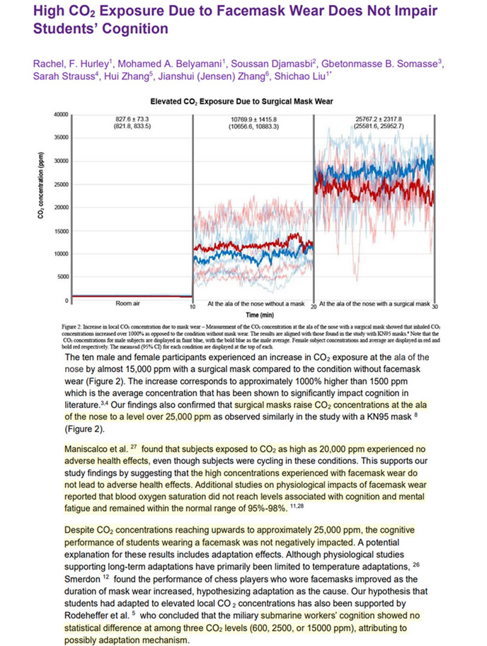
[Here is a paper about climate sensitivity (CS) to a perturbation to Earth’s Energy Imbalance. The observed CS is -0.4°C per -9 W/m² (0.044°C per W/m²). This means a +75 W/m² perturbation is required to produce the alleged GMST response (3.3°C) to 2xCO2.]
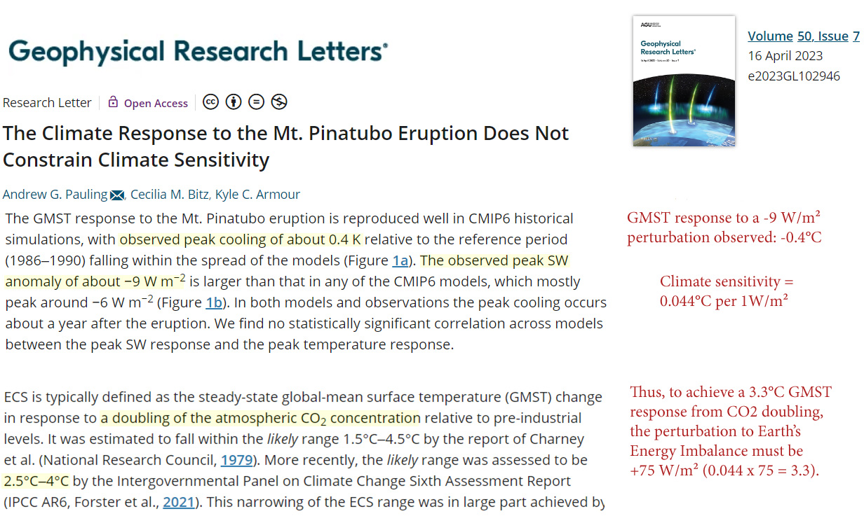


Recent Comments