Scafetta and Willson, 2019 The consistent downward trending of the PMOD TSI composite is negatively correlated with the global mean temperature anomaly during 1980–2000. This has beenviewed with favor by those supporting the CO2 anthropogenic global warming (CAGW) hypothesis since it would minimize TSI variation as a competitive climate change driver to CO2, the featured driver of the hypothesis during the period (cf.: [IPCC, 2013, Lockwood and Fröhlich, 2008]). .. Our summary conclusion is that the objective evidence produced by all of the independent TSI composites [3,5, 6, 9] agrees better with the cycle-by-cycle trending of the original ACRIM science team’s composite TSI that shows an increasing trend from 1980 to 2000 and a decreasing trend thereafter. The continuously downward trending of the PMOD composite and TSI proxy models is contraindicated. … PMOD’s modifications of the published ACRIM and ERB TSI records are questionable because they are based on conforming satellite observational data to proxy model predictions. … ACRIM shows a 0.46 W/m2 increase between 1986 and 1996 followed by a decrease of 0.30 W/m2 between 1996 and 2009. PMOD shows a continuous, increasing downward trend with a 1986 to 1996 decrease of 0.05 W/m2 followed by a decrease of 0.14 W/m2 between 1996 and 2009. The RMIB composite agrees qualitatively with the ACRIM trend by increasing between the 1986 and 1996 minima and decreasing slightly between 1996 and 2009. … ACRIM composite trending is well correlated with the record of global mean temperature anomaly over the entire range of satellite observations (1980–2018) [Scafetta. 2009]. The climate warming hiatus observed since 2000 is inconsistent with CO2 anthropogenic global warming (CAGW) climate models [Scafetta, 2013, Scafetta, 2017]. This points to a significant percentage of the observed 1980–2000 warming being driven by TSI variation [Scafetta, 2009, Willson, 2014, Scafetta. 2009]. A number of other studies have pointed out that climate change and TSI variability are strongly correlated throughout the Holocene including the recent decades (e.g., Scafetta, 2009, Scafetta and Willson, 2014, Scafetta, 2013, Kerr, 2001, Bond et al., 2001, Kirkby, 2007, Shaviv, 2008, Shapiro et al., 2011, Soon and Legates, 2013, Steinhilber et al., 2012, Soon et al., 2014). .. The global surface temperature of the Earth increased from 1970 to 2000 and remained nearly stable from 2000 and 2018. This pattern is not reproduced by CO2 AGW climate models but correlates with a TSI evolution with the trending characteristics of the ACRIM TSI composite as explained in Scafetta [6,12, 27] and Willson [7].
Pei et al., 2019 During the period of 0–10,000 yr BP, China’s temperature has closely followed the solar forcing. The correlation is as high as 0.800 (p < 0.01) for the EOF-based reconstruction. … Similar to the North Atlantic SST, AO also plays an important role in China’s temperature (Zuo et al., 2015). NAO and AO are both suggested to influence the climate in East Asia by modifying the strength and location of the 200 hPa jet stream (Yang et al., 2004). The AO record of Darby et al. (2012) is based on sea-ice drift, which has a high resolution of 10–100 years and shows a close connection with solar activities.
Lüning et al., 2019 Modern climate variability in Oceania is heavily influenced by El Niño-Southern Oscillation, ENSO (e.g. McLean et al., 2009; Ning et al., 2018; Wang et al., 2017), Indian Ocean Dipole, IOD (e.g. Zhang et al., 2015), Southern Annular Mode, SAM (e.g. Gillett et al., 2006), and the Interdecadal Pacific Oscillation, IPO (e.g. Duncan et al., 2010; Salinger et al., 2014). Palaeoclimate reconstructions of the past centuries and millennia have identified such cycles as important climatic drivers (Cook et al., 2000; Cook et al., 2006; Gouramanis et al., 2013; Komugabe‐Dixson et al., 2016; Lorrey et al., 2008; Perner et al., 2018). The main MCA warming phase coincides with a higher SAM, more El Niño-dominated ENSO, more positive IPO and higher solar activity (Abram et al., 2014; Conroy et al., 2008; Steinhilber et al., 2012; Vance et al., 2015) (Fig. 5). Spectral analysis of the classical Mt Read tree rings series (site 5), yields characteristic cycle periods associated with the solar Gleissberg (80 years) and Suess-de Vries (210 years) cycles (Cook et al., 1995; Cook et al., 2000). … An alternation of well-defined multicentennial warm and cold phases has been reconstructed for Grotto of Oddities in SE Australia (site 3). Temperatures oscillated with an amplitude of more than 1°C during the past 1500 years (McGowan et al., 2018).
Kasatkina et al., 2019 The analysis revealed significant cooling events, coinciding with the Spoerer (1400–1540), Maunder (1645–1715), Dalton (1790–1830), and Gleissberg (1880–1910) Grand Solar Minima. The application of MTM-spectrum and wavelet decomposition analysis identified the existence of the main cycles of solar activity (5.4, 11.7 and 22 years) in tree-ring width variations. As possible extraterrestrial forcings of climate change we consider here variations in solar irradiance and cosmic ray intensity modulated by the interplanetary magnetic field. As solar and cosmic ray activity indicators we used the annual sunspot number, geomagnetic aa index and Be^10 cosmogenic isotope records. To examine the relationship in time-frequency scale between tree-ring growth and solar activity, the cross wavelet transform and wavelet coherence analysis were applied to the time series. The wavelet coherence analysis identified that the 11 yr and 22 yr periodicities were clearly manifested in the all solar-tree rings connections during and around the Grand Minima of solar activity including the Maunder minimum, when, as is known, sunspots were practically absent. These results confirm the existence of solar activity effect on climate and tree growth above the Arctic Circle and are important for understanding the modern climatic processes.
Frederick et al., 2019 Downward longwave radiation measured at Alert, Canada, shows responses to the interplanetary magnetic field. Upward longwave radiation responds similarly a day later. The phenomenon is consistent with solar wind inputs to atmospheric electricity affecting cloud microphysics. … These results are qualitatively consistent with a previously proposed mechanism in which the interplanetary magnetic field perturbs the ionosphere-to-ground potential difference and the downward atmospheric current density over limited regions near the geomagnetic poles, altering local cloud properties. We find that the atmospheric longwave emission is altered on a time scale of 3 days, with a change in surface temperature appearing one day later, attributable to the thermal inertia of the surface. When one moves from the geomagnetic latitude of Alert (3° from the north geomagnetic pole) to the latitude of Barrow (∼20° from that pole), any connection between By [interplanetary magnetic field] and longwave irradiance becomes too small to isolate from the natural background variability.
Veretenenko and Ogurtsov, 2019 Temporal behavior of correlation coefficients between troposphere pressure at extratropical latitudes and sunspot numbers was compared with long-term changes in the evolution of large-scale circulation, the intensity of the stratospheric polar vortex and global temperature anomalies. It was shown that a roughly 60-year periodicity revealed in solar activity influences on troposphere pressure (development of extratropical baric systems) is closely related to changes in the large-scale circulation regime which accompany transitions between strong and weak states of the stratospheric polar vortex. It was suggested that the detected correlation reversals are caused by changes of the troposphere-stratosphere coupling associated with changes of the vortex intensity. It was shown that the changes of the polar vortex state and the corresponding changes in the regime of large-scale circulation may be related to global temperature variations, with a possible reason for these variations being long-term changes of total solar irradiance.
Scafetta et al., 2019 By adjusting the TSI proxy models to agree with the data patterns before and after the ACRIM-gap, we found that these models miss a slowly varying TSI component. The adjusted models suggest that the quiet solar luminosity increased from the 1986 to the 1996 TSI minimum by about 0.45 W/m2 reaching a peak near 2000 and decreased by about 0.15 W/m2 from the 1996 to the 2008 TSI cycle minimum. This pattern is found to be compatible with the ACRIM TSI composite and confirms the ACRIM TSI increasing trend from 1980 to 2000, followed by a long-term decreasing trend since. … This model was extended using the ACRIM composite since 1981 and an average between VIRGO and SORCE TIM since 2013. This particular TSI model appeared to correlate well with the Earth’s global surface temperature records since 1700 [Hoyt et al., 1993, . … The TSI data from 1978 to 1981 appeared too corrupted because of uncorrected degradation of theNimbus7/ERB sensors during the solar maximum of cycle 21. For this reason, it was more appropriate to dismiss the data from this period because modifying TSI data using proxy models, as done by PMOD, would be arbitrary. We proposed that any reliable TSI composite should begin from late 1980 with the ACRIM1 record. … The same harmonic solar model suggests that the sun may now be heading toward a new grand solar minimum in the 2030–2040 time frame. Final evidence that TSI may have increased from 1980 to 2000 comes from Earth’s climate studies. Secular climate records correlate well with TSI curves such as the one depicted in Figure 13 and on longer ones covering the entire Holocene [1,23,60,64]. In particular, the warming observed from 1970 to 2000, followed by a temperature standstill since 2000, is a good fit for a natural 60-year cycle prediction superimposed to other contributions [20]. This pattern correlates better with a TSI evolution similar to the ACRIM composite [17–21,62,65] than with the CMIP5 general circulation climate model predictions of continuous anthropogenic warming [22]. The CMIP5 climate models use a high climate sensitivity to CO2 forcing and low secular TSI variability proxy models, such as the one proposed in [3], which was calibrated using the PMOD TSI composite model after 1980.
Spiridonov et al., 2019 The Earth’s biota originated and developed to its current complex state through interacting with multilevel physical forcing of our planet’s climate and near and outer space phenomena. In the present study, we focus on the time scale of hundreds to thousands of years in the most recent time interval – the Holocene. Using a pollen paleocommunity dataset from southern Lithuania (Čepkeliai bog) and applying spectral analysis techniques, we tested this record for the presence of statistically significant cyclicities, which can be observed in past solar activity. The time series of non-metric multidimensional scaling (NMDS) scores, which in our case are assumed to reflect temperature variations, and Tsallis entropy-related community compositional diversity estimates q* revealed the presence of cycles on several time scales. The most consistent periodicities are characterized by periods lasting between 201 and 240 years, which is very close to the DeVries solar cycles (208 years). A shorter-term periodicity of 176 years was detected in the NMDS scores that can be putatively linked to the subharmonics of the Gleissberg solar cycle. In addition, periodicities of ≈3,760 and ≈1,880 years were found in both parameters. These periodic patterns could be explained either as originating as a harmonic nonlinear response to precession forcing, or as resulting from the long-term solar activity quasicycles that were reported in previous studies of solar activity proxies.
Jiao et al., 2019 Regional climate change is affected by large-scale climate-forcing factors, such as solar activity and atmospheric–oceanic variability (Fang et al., 2010; Linderholm et al., 2015; Rydval et al., 2017). On the one hand, based on the MTM analysis results, the temperature changes in the study area are mainly influenced by the solar activity via the mean minimum temperature within approximately 11-year periods (Li et al., 2006; Wang et al., 2015). The tree-ring chronology was developed by samples of Schrenk spruce collected from the National Nature Reserve of the Western Tianshan Mountains. The mean minimum temperature in the growing season is the main and stable limiting climate factor. Therefore, the mean minimum temperature series in the growing season during 1680–2012 was reconstructed based on the STD chronology. In the past 333 years, the mean minimum temperature has roughly experienced three relatively cold periods and relatively warm stages (relatively cold periods: 1680–1707, 1802–1911 and 1935–1997; relatively warm periods: 1708–1801, 1912–1934 and 1998–2012). By analyzing similar trends in regional temperature changes in our reconstruction series with drought events, large volcanic eruptions and other reconstruction series around the study regions in Xinjiang and even large-scale regions, wefound that the mean minimum temperature of the reconstruction was accurate and reliant. Moreover, the mean minimum temperature was influenced by solar activity (sunspots) and large-scale atmospheric–oceanic fluctuations (NAO, WPO, ENSO, TBO) based on the MTM and spatial correlation analysis.
Zharkova et al., 2019Recently discovered long-term oscillations of the solar background magnetic field associated with double dynamo waves generated in inner and outer layers of the Sun indicate that the solar activity is heading in the next three decades (2019–2055) to a Modern grand minimum similar to Maunder one. On the other hand,a reconstruction of solar total irradiance suggests that since the Maunder minimum there is an increase in the cycle-averaged total solar irradiance (TSI) by a value of about 1–1.5 Wm−2 closely correlated with an increase of the baseline (average) terrestrial temperature. … These oscillations of the baseline solar magnetic field are found associated with a long-term solar inertial motion about the barycenter of the solar system and closely linked to an increase of solar irradiance and terrestrial temperature in the past two centuries. This trend is anticipated to continue in the next six centuries that can lead to a further natural increase of the terrestrial temperature by more than 2.5 °C by 2600.
Deke et al., 2019 The results provide robust evidence for synchronous ~500-yr cyclical changes in monsoon climate, human activity and prehistoric cultural development in the East Asian Monsoon (EAM) region during the Holocene. Six prosperous phases of Neolithic and Bronze Age cultures correspond approximately to warm-humid phases caused by a strengthened EASM, except for the first expansion of the Hongshan culture, which corresponds to the phase of strongest EASM in the middle Holocene. We suggest that humans responded to climatic fluctuations with different social strategies, leading to the rise and fall of early complex societies in the region.
(press release) The climate theory casting new light on the history of Chinese civilisation … Researchers say that when 500-year-long sun cycles brought warmth, communities flourished, but when the Earth cooled, ancient societies collapsed. … Scientists say they have found evidence beneath a lake in northeastern China that ties climate change and 500-year sun cycles to ups and downs in the 8,000 years of Chinese civilisation. According to the study by a team at the Institute of Geology and Geophysics in Beijing published in the science journal Nature Communications this month, whenever the climate warmed, Chinese civilisation prospered and when it cooled, it declined.
Jin et al., 2019 We show that a strong 11-year solar cycle can excite a resonant response of the intrinsic leading mode of the AWM [Asian winter monsoon] variability, resulting in a significant signal of decadal variation. The leading mode, characterized by a warm Arctic and cold Siberia, responds to the maximum solar irradiance with a peculiar 3 to 4-year delay. We propose a new mechanism to explain this delayed response, in which the 11-year solar cycle affects the AWM via modulating Arctic sea ice variation during the preceding summer. At the peak of the accumulative solar irradiance (i.e., 4 years after the maximum solar irradiance), the Arctic sea ice concentration reaches a minimum over the Barents–Kara Sea region accompanied by an Arctic sea surface warming, which then persists into the following winter, causing Arctic high-pressure extend to the Ural mountain region, which enhances Siberian High and causes a bitter winter over the northern Asia.
Horikawa et al., 2019 The Mg/Ca-derived SST record clearly represented five warmer periods at 6200–6000, 4900–4500, 4200–3800, 2600–2100, and 900–400 cal. year BP, almost consistent with previously published diatom records. These warmer events also corresponded to the periods in which warm molluscan assemblages increased at the northern end of the TWC, suggesting that periods of higher SST can be seen as reflecting the increased volume transport of the TWC. We interpreted the results of a model study showing that higher solar irradiance provoked positive Arctic Oscillation (AO)-like spatial patterns and the negative phase of the Pacific Decadal Oscillation (PDO) to mean that increased (reduced) TWC volume transport on the multi-centennial to millennial time scales was caused by high (low) solar insolation via a potential link between AO and PDO.
Kossobokov et al., 2019On the Diversity of Long-Term Temperature Responses to Varying Levels of Solar Activity at Ten European Observatories … In the present paper, we propose a short but in-depth overview of a very specific topic, i.e., the statistical testing of hypotheses related to solar influence on regional temperature regimes at the time scale of several decades. … These new observations lead us to conclude that the climate in different regions presents different responses to variations in solar activity. Moreover, the distributions of the lower, middle, and higher quartiles of the temperature and pressure indices in solar cycles with high versus low activity are significantly different, providing further robust statistical confirmation to this conclusion (confidence level higher to much higher than 99% using the Kuiper test).
Wu et al., 2019 On the centennial to millennial time scale, the results of wavelet analysis and band‐pass filtering show that the occurrence and development of El Niño have also promoted a weaker EAWM after ~6.0 ka cal. BP, which is inversely correlated with the variation of the ca. 500‐year cycle originated from changes in solar output. These results imply that the climate transition in the mid‐Holocene is caused by the change of variations in solar activity and amplified by ocean circulation El Niño‐Southern Oscillation to influence the East Asian Monsoon system, especially the EAWM, and finally change the vegetation in Great Khingan Mountain Range.
(press release) Lead scientist Dr Wu Jing, from the Key Laboratory of Cenozoic Geology and Environment at the Institute of Geology and Geophysics, part of the Chinese Academy of Sciences, said the study had found no evidence of human influence on northern China’s warmingwinters. … The study found that winds from Arctic Siberia have been growing weaker, the conifer tree line has been retreating north, and there has been a steady rise in biodiversity in a general warming trend that continues today. It appears to have little to do with the increase in greenhouse gases which began with the industrial revolution, according to the researchers. As a result of the research findings, Wu said she was now more worried about cooling than warming.
Wang et al., 2019Here we present the first high-resolution stable isotope (δ13C and δ18O) speleothem record from northern Laos spanning the Common Era (∼50 BCE to 1880 CE). The δ13C record reveals substantial centennialscale fluctuations primarily driven by local water balance. Notably, the driest period at our site occurred from ∼1280 to 1430 CE, during the time of the Angkor droughts, supporting previous findings that this megadrought likely impacted much of Mainland Southeast Asia. In contrast, variations in stalagmite δ18O reflect changes in rainfall upstream from our study site. Interestingly, the δ18O record exhibits a positive correlation with solar activity that persists after 1200 CE, contrary to the findings in previous studies. Solar-forced climate model simulations reveal that these δ18O variations may be driven by solar-forced changes in upstream rainout over the tropical Indian Ocean, which modify the δ18O of moisture transported to our study site without necessarily affecting local rainfall amount. We conclude that future rainfall changes in Mainland Southeast Asia are likely to be superimposed on multi-decadal to centennial-scale variations in background climate driven primarily by internal climate variability, whereas solar forcing may impact upstream rainout over the Indian Ocean.
Misios et al., 2019 The Pacific Walker Circulation (PWC) fluctuates on interannual and multidecadal timescales under the influence of internal variability and external forcings. Here, we provide observational evidence that the 11-y solar cycle (SC) affects the PWC on decadal timescales. We observe a robust reduction of east–west sea-level pressure gradients over the Indo-Pacific Ocean during solar maxima and the following 1–2 y. This reduction is associated with westerly wind anomalies at the surface and throughout the equatorial troposphere in the western/central Pacific paired with an eastward shift of convective precipitation that brings more rainfall to the central Pacific. We show that this is initiated by a thermodynamical response of the global hydrological cycle to surface warming, further amplified by atmosphere–ocean coupling, leading to larger positive ocean temperature anomalies in the equatorial Pacific than expected from simple radiative forcing considerations. The observed solar modulation of the PWC is supported by a set of coupled ocean–atmosphere climate model simulations forced only by SC irradiance variations. We highlight the importance of a muted hydrology mechanism that acts to weaken the PWC. Demonstration of this mechanism acting on the 11-y SC timescale adds confidence in model predictions that the same mechanism also weakens the PWC under increasing greenhouse gas forcing.
Bhargawa and Singh, 2019 Since the Sun is the main source of energy for our planet therefore even a slight change in its output energy can make a huge difference in the climatic conditions of the terrestrial environment. The rate of energy coming from the Sun (solar irradiance) might affect our climate directly by changing the rate of solar heating of the Earth and the atmosphere and indirectly by changing the cloud forming processes. … In our investigation, we have observed that the impact of solar irradiance on the global surface temperature level in next decade will increase by ∼4.7% while the global mean sea level will increase about 0.67%. In the meantime, we have noticed about 5.3% decrement in the global sea-ice extent for the next decade. In case of the global precipitation anomaly we have not observed any particular trend just because of the variable climatic conditions. We also have studied the effect of CO2 as anthropogenic forcing where we have observed that the global temperature in the next decade will increase by 2.7%; mean sea level will increase by 6.4%. Increasing abundance in CO2 will be responsible for about 0.43% decrease in the sea-ice extent while there will not be any change in the precipitation pattern.
Zaffar et al., 2019 This study shows that every value of El Nino-southern oscillation (ENSO) Cycles and Sunspot Cycles are strongly correlated to preceding values in both the self-similar and self-affine cases. Unit root test is applied to the tail parameter and the strength of long range-correlation of El Nino-southern oscillation (ENSO) and Sunspot Cycles confirms stationary behavior of the parameters. Thevariation of earth climatic has a strong influence in Sunspots Cycles and El Nino-southern oscillation (ENSO) Cycles. Sunspots and El Nino-southern oscillation (ENSO) have strong correlation with each other (Asma et al. 2018). The El Nino-southern oscillation (ENSO) cycles influence on the variation of the parameter of local climate which depends on the changes in solar activity.
Maliniemi et al., 2019Here we study how December to February climate is affected by two solar‐related drivers, geomagnetic activity (proxy of particle precipitation) and sunspot activity (proxy of solar UV) during 1948‐2017. … Geomagnetic activity produces a strengthening of the polar vortex and a negative poleward SLP gradient between mid‐ and high latitudes, resembling a positive NAO‐type circulation pattern during December to February. Solar UV produces a positive U anomaly in the low‐latitude stratosphere during December, which moves poleward and downward during the winter resulting a negative poleward SLP gradient between mid‐ and high latitudes during February. We find the lagged sunspot activity responses in SLP to form zonal pressure patterns (wave‐train structure) resembling the Eurasian pattern. Geomagnetic activity responses remain essentially the same when we introduce the lag with respect to sunspot activity supporting its independency as a driving mechanism. Our results suggest that solar wind related particle precipitation and (lagged) solar UV mechanism provide independent, significant circulation signals in the North Atlantic winter.
Sun et al., 2019 The results show that the hydroclimate was generally humid during 7.57–4.65 cal ka BP, and that subsequently it became relatively dry during 4.65–1.37 cal ka BP. Our results also reveal that the centennial scale variability of the lake level during the Holocene is forced by changes in solar activity and oceanic–atmospheric feedback.
Feng et al., 2019 The wavelet and Redfit analyses of δ18O showed 97, 61, and 35 a signals in the 8.0–7.0 ka BP period, which were similar to the Gleissberg solar and the AMOC cycles. Among these, the 61 a cycle was the most significant. Combined with paleoclimatic geological records, the sea level rose after 8.0 ka BP due to the large-scale melting of ice sheets in the high latitudes of the Northern Hemisphere. The intensity of solar activity has gradually become the main driving mechanism of climate change in the Northern Hemisphere. In addition, the meridional overturning circulation anomaly of seawater in high latitudes and the movement of ITCZ between the Northern and Southern Hemispheres in low latitudes will amplify the impact of solar activity on the climate system, thereby triggering anomalies in the Northern Hemisphere monsoon circulation such as the ‘7.2 ka event’.
Han et al., 2019 The wavelet and RQA analyses of dust activity records from both the TB and Greenland areas indicate similar system changes and a possible control of solar activity on dust activity in both areas. … Steepening of the latitudinal temperature gradient caused by the combined effects of the longterm decrease/ increase in Arctic summer/mid-latitude winter insolation and a change in solar activity is suggested as an important factor driving the transition of the environmental system at ~4.4 kyr BP with full establishment of an unstable new system after 3.5 kyr BP that is characterized by dust storms outbreak in central Asia. Increased low level wind intensity and a delayed seasonal jet transition, resulting from intensification and a southward shift of the westerly jet during cold periods, were key in keeping central Asia in conditions favoring an increase in dust activity.
Ding et al., 2019 [T]he climate of 8.3~4.2 ka BP is moderately warm and humid, 4.2~2.3 ka BP is dry and cold, the climate has warmed since 2.3 ka BP, and the significant climate cycle of 238 a indicates that solar activity has an important impact on regional climate since the Holocene. Using the benthic foraminifera δ 18 O, Mg/Ca value, magnetic susceptibility, Al/Ti, Ba/Ti, etc., the 3-4, 7.2, and 6.2 ka three-time cooling events were identified in the Middle Holocene , with a range of 200 a. The cycle is most pronounced, presumably related to solar activity.
Jiang et al., 2019 In this study, ring-width chronology of Picea jezoensis var. microsperma from the Changbai Mountain (CBM) area, Northeast China, was constructed. … The reconstructed temperature series corresponded to the historical disaster records of extreme climatic events (e.g., drought and flood disasters) in this area. … It is widely believed that the climate will get colder in periods of less solar activity (e.g., the “Little Ice Age” during AD 1450 and 1850), while in a period of intense solar activity, the climate will become warmer (e.g., the warm period of the Middle Ages during AD 1000 and 1400). … [M]ulti-taper method spectral analysis indicated the existence of significant periodicities in the reconstructed series. The significant spatial correlations between the reconstructed temperature series and the El Niño–Southern Oscillation (ENSO), solar activity, and Pacific Decadal Oscillation (PDO) suggested that the temperature in the CBM area indicated both local-regional climate signals and global-scale climate changes. … The 11-year smoothing average of the reconstructed Tmax6–7 series was used to reveal low-frequency information and to show temperature variability in this area. After smoothing with an 11-year moving average, cold periods occurred in 1899–1913 (average value was 21.41 °C), 1955–1970 (21.49 °C), and 1975–1989 (20.97 °C), while warm periods occurred in 1881–1888 (23.93 °C). Furthermore, there are six obvious processes of Tmax6–7 increasing in 1781–1791 (from 22.76 °C to 23.54 °C), 1800–1809 (from 22.72 °C to 23.44 °C), 1835–1845 (from 22.66 °C to 23.76 °C), 1900–1919 (from 21.47 °C to 22.30 °C), 1931–1942 (from 21.36 °C to 22.04 °C), and 1983–2004 (from 20.49 °C to 22.99 °C), and five obvious processes of Tmax6–7 decreasing in 1790–1800 (from 21.89 °C to 22.98 °C), 1810–1835 (from 23.40 °C to 22.66 °C), 1880–1901 (from 23.83 °C to 21.25 °C), 1917–1931 (from 22.36 °C to 21.36 °C), and 1970–1983 (from 21.75 °C to 20.49 °C). In addition,the temperatures during 1780–1890 were much warmer (average value was 23.35 °C) than the temperatures during 1900–2004 (average value was 21.65 °C).
Moreno et al., 2019 Spectral and wavelet transform coherence analyses were used to detect solar footprints on foraminiferal and climate-related time series. A main significant quasi-periodicity was identified within the range of the secular Gleissberg cycle ofsolar activity modulating the annual NAO and regional spring-summer (simulated) temperatures after AD 1700. This stronger solar-climate coupling may be related to the known upward secular trend in the total solar irradiance after the Maunder Minimum.
Zhao et al., 2019 TSI provides nearly 99.96% of the energy driving Earth climate and its 0.15% variation has a great influence (Kren 2015). Moreover, not only does TSI vary by about 0.01%, caused by the several-minutes-long continuous change from the solar convection zone to the photosphere, it also varies by about 0.3% over 300 years (Eddy 1976). Besides TSI, solar wind is another solar activity, which consists of three types based on the different velocity, extremely high-velocity (v≥725 km/s), high-velocity (450≤v<725 km/s) and low-velocity (v<450 km/s) wind. While TSI is an important observable factor in solar activity variation, a lot of weather and climate models attempt to attribute it as a physically important factor when trying to understand whether and how the Sun has an impact on the Earth’s weather and climate (Scafetta 2010; Coddington et al. 2016). Beyond the widely known quasi 11-year and century periods, Mendoza (2005) concluded that the TSI fluctuations on the 5 min range are due to solar oscillations (Fröhlich et al. 1997; Wolff and Hickey 1987), while few days to weeks are dominated by sunspots (Chapman 1987), and faculae can enhance the total flux by 0.08% (Hudson et al. 1982). Apart from the intrinsic longand short-term variations of TSI, the changes of the Earth’s orbital parameter and albedo cause the variations of the solar electromagnetic radiation that arrives at the Earth (Mendoza 2005). The radiation, especially in the UV bands influenced by the short but strong solar activity (e.g., flare, coronal mass ejection), affects the temperature variation that plays a key role in climate change (Smith et al. 1990).
Li et al., 2019 The result obtained by analyzing that quasiperiodicity shows that the main periods of tree ring width and the sunspot number in the same period are basically consistent, and tree ring width has other cycles. This shows that sunspot activity is an important factor affecting tree ring growth, and tree ring width is influenced by other external environments. … The influence of solar activity on climate has attracted much attention as early as the seventeenth century. Solar activity is an important controlling factor of the earth’s climate. It plays a leading role in the earth’s climate change[1]. Many research studies [2–4] have shown that solar activity is closely related to natural environment changes such as temperature and various dust storms, floods, and droughts.
Zherebtsov et al., 2019We address the solar activity effect on the changes in the temperature of the atmosphere and of the World Ocean. … We revealed the regions, where long-term SST changes are determined mainly by SA [solar activity] variations. … Comparing variations in climate and solar activity reveals great similarity in their behavior on large time scales. In particular, there are reasonable grounds to believe that the periods of cooling and warming (at least, in the previous millennium) were precisely related to the solar activity variations. Over recent 1000 years, climate has undergone the changes that corresponded to the solar activity variations: warming was recorded in the 12–13th centuries, when solar activity was high (“Medieval Climatic Optimum”), and two temperature drops in the Little Ice Age (in the 16–17th centuries) corresponded to long periods of low solar activity (Dalton and Maunder Minima) (Fig. 1). After the Maunder Minimum, solar activity increase has been widely observed. So, the world climate has become warmer during the bulk of this period. … Earlier, the authors (Kirichenko et al., 2014) analyzed the long-term variations in the SST spatial distribution and in geomagnetic activity. As a result, we found a relation between the SST changes and the geomagnetic activity variations. The SST response to geomagnetic effects was established to feature a significant spatial time irregularity and has a regional character. … Based on the complex analysis of the hydro-meteorological observational data and the authors’ model for the solar activity effect on the climate system, we obtained new evidence for the SA [solar activity] effect on the weather-climate characteristics in the troposphere and in the ocean, including the surface air temperature and the ocean surface temperature. … We calculated the temperature vertical profile variations within the troposphere during heliogeophysical disturbances. The troposphere temperature response to individual heliogeophysical disturbances is shown to be accompanied by the temperature field regular change. In the regions of the temperature maximal response to heliogeophysical disturbances in the middle and in the lower troposphere, one observes a significant (up to 15°) temperature increase. … We found the regions, in which long-term variations in the ocean surface temperature are mainly determined by geomagnetic activity variations. Along with this, the wind stress direction variations were revealed to affect the manifestation of the solar-geomagnetic effect on the ocean surface temperature. They lead to a “hiatus” in the relation between the ocean surface temperature and solar activity due to the change in the ocean thermodynamic state because of the vertical mixing increase.
Deininger et al., 2019 A centennial periodicity of the SAMS [South American Monsoon System] (around 210 years) was reported from different sites and is associated with the de Vriess–Suess solar cycle, exhibiting depleted δ18O during periods of high solar irradiance. It is proposed that this relationship is due to several feedbacks involving amplification of solar forcing by coupled air-sea dynamics, cloud formation and stratospheric warming due to enhanced UV absorption through increased stratospheric ozone concentration. … The proposed mechanism driving the Botuverá δ18O record in southeast Brazil is intensification of the SAMS [South American Monsoon System], as driven by increasing austral summertime insolation, suggesting a progressive increase in precipitation amount throughout the Holocene.The main climate features over the last two millennia in South America were forced by NH warm and cold periods during the Medieval Climate Anomaly (MCA) and the Little Ice Age (LIA), respectively. … During the CWP [current warm period], the convective conditions over South America appear to be similar to the MCA [Medieval Climate Anomaly], with warming in the NH leading to a northward positioning of ITCZ and a progressive weakening of the SAMS.
Ball et al., 2019The solar cycle (SC) stratospheric ozone response is thought to influence surface weather and climate. To understand the chain of processes and ensure climate models adequately represent them, it is important to detect and quantify an accurate SC ozone response from observations. Chemistry climate models (CCMs) and observations display a range of upper stratosphere (1–10 hPa) zonally averaged spatial responses; this and the recommended dataset for comparison remains disputed. Recent data‐merging advancements have led to more robust observational data. Using these data, we show that the observed SC [solar cycle] signal exhibits an upper stratosphere U‐shaped spatial structure with lobes emanating from the tropics (5–10 hPa) to high altitudes at mid‐latitudes (1–3 hPa). We confirm this using two independent CCMs in specified dynamics mode and an idealised timeslice experiment. We recommend the BASICv2 ozone composite to best represent historical upper stratospheric solar variability, and that those based on SBUV alone should not be used.
Kusch et al., 2019 The Holocene climate history of the high-Arctic has largely been driven by the decline in summer insolation (Berger & Loutre 1991; Kaufman et al. 2004) amplified by oceanic and atmospheric feedbacks, most importantly an increased meridional heat and moisture transfer, as well as volcanic forcing (Briner et al. 2016; Kobashi et al. 2017; Lecavalier et al. 2017). Mean summer insolation at 80°N was approximately 50 W m-2 higher during the Early Holocene (Greenlandian) insolation maximum compared to today and resulted in the Early to Middle Holocene thermal maximum (HTM) causing retreat and disappearance of the northern ice sheets except for the Greenland Ice Sheet (Berger & Loutre 1991; Ullman et al. 2015). … Most records, including ice-cores and sedimentary archives, document the HTM between approximately 9 and 5 cal. ka BP with average temperature anomalies of 2.5 to 3.0 °C [higher than today] (Briner et al. 2016) in agreement with climate models (e.g. Renssen et al. 2012).
Ansor et al., 2019 The amount of solar radiation absorbed and reflected determine the rising or declining in Earth’s climate. Generally, Earth’s system absorbs 71% of total incoming solar radiation and 29% is reflected back. When atoms and molecules absorb energy, the matter become excited and moves quickly and randomly and leads to increase in the matter’s temperature. If more energy is absorbed, more particles increase in temperature and eventually Earth’s atmosphere and surface start to warm up. The origin of this result goes back to Sun’s temperature, where, the hotter the Sun is, more solar energy is produced leads to high incoming energy absorbed by Earth. Meanwhile, the temperature of the Sun is based on the presence of sunspots; less sunspot number, [the] hotter the Sun will be. … Overall, this article reviews some evidences from previous studies and we present solar activity data throughout 2017 during solar minimum to prove the possibility of solar radiation emitted by solar flares and coronal mass ejections in changing Earth’s climate pattern. By gathering the data records, we believe climate change is contributed by the variability of solar activity, in which, solar minimum results in high solar radiation produced and received by the Earth. Hence, less amount of energy absorbed results in low of the Earth’s temperature.
Yan et al., 2019 We contend that solar activity and the westerlies were the dominant influences on ACA [arid central Asia] hydroclimatic variations during the period of record [the last 160 years]: (1) solar activity dominates regional temperature variations, precipitation/evaporation, and the advance/retreat of glaciers; (2) stronger westerly intensity (corresponding to higher westerly index and higher North Atlantic Oscillation (NAO) index) brings more water vapor from the west to ACA [arid central Asia], and vice versa; and (3) the southerly migration of the westerly jet stream, which is closely related to lower TSI and temperatures, could favor more water vapor transported to ACA areas, and vice versa.
Nitka and Burnecki, 2019 In this paper we analyze the relationship between the sunspot numbers and the average monthly precipitation measured at meteorological stations in the US. The results indicate that there is a significant correlation between the solar activity and the monthly average precipitation data for selected months and time delays.
Huang et al., 2019 [T]hese events are synchronous with periods of weak solar activity, and the spectral analysis demonstrates that the EASM and solar activity share some general cyclicity patterns. We therefore suggest that solar activity is a fundamental driving force for the spatial synchronisation of the EASM [East Asian Summer Monsoon] on centennial timescales across the monsoon region. … The sun-monsoon link can be explained by a direct solar influence on the land–sea thermal contrast that controls the monsoonal precipitation (Liu et al., 2009; Xu et al., 2015). When the land–sea thermal contrast reduces, the subsequent gradual southward migration of the Intertropical Convergence Zone (ITCZ) may lead to reduced transportation of water vapor from the ocean to the continents, thereby causing less rainfall in monsoonal Asia (Dykoski et al., 2005; Fleitmann et al., 2003; Li et al., 2017b). In general, weak solar activity triggers decreased land–sea thermal contrast, and thereafter would result in reductions in the EASM intensity. Alternately, solar output could influence the variability of the EASM indirectly, perhaps amplified by the North Atlantic teleconnection (Wang et al., 2005, 2016).
Liu et al., 2019 Notably, an overall in‐phase relationship is observed between the hydroclimatic variations and change in solar activity, and the results of spectral analysis suggest the presence of the Eddy (~1080 yr), de Vries (~205 yr) and Gleissberg (~88‐102 yrs) cycles. This indicates a linkage between solar activity and hydroclimatic changes in ACA [arid Central Asia] on centennial‐ to multi‐decadal scales during the Holocene. We suggest that the influence of solar activity on hydroclimatic changes in ACA [arid Central Asia] occurs via its effects on North Atlantic sea surface temperature (SST), North Atlantic Oscillation (NAO), northern high‐latitude regional temperatures, and via direct heating. The relationship suggests that solar activity may play an important role in determining future hydroclimatic changes in ACA[arid Central Asia].
Banerji et al., 2019The present study demonstrates vacillating climate with strengthened ISM [Indian Summer Monsoon] during Roman Warm Period and Medieval Warm Period (2000−950 cal yr BP) as a result of increased solar irradiance interrupted by reduced ISM during Dark Ages of Cold Period (∼1500 cal yr BP). The plausible occurrence of volcanic eruption before the onset of Little Ice Age (500−200 cal yr BP) resulted the southward migration of ITCZ leading to enhanced western disturbances in the study area thereby causing cool and wet climate. The study also emphasis the increased El Nino events with gradual decline in the ISM since LIA. Further, the study underscores a climate warming during last two centuries which corroborated well with the instrumental records. Thus, the present study has implication towards understanding the significant role of volcanic activity and solar variability in controlling the millennia scale climate oscillations with additional feedback mechanisms.
Cho et al., 2019[T]he EASM [East Asian Summer Monsoon] was weak during the LIA, and the amount of precipitation was lower than in other periods. ENSO is strongly related to sea surface temperature (SST) in the Pacific Ocean (Schwing et al., 2002; Marchitto et al., 2010). This SST is also affected by solar activity. Marchitto et al. (2010) showed that proxy-based SST records based on Mg/Ca ratio correlated with the generation of cosmogenic nuclides 14C and 10Be. Therefore low solar activity is correlated with El Niño-like conditions (Marchitto et al., 2010). Japan has a complicated climate system, but it is one that is closely related to solar insolation. The climate of Japan over the last 1000 years has undergone significant variation. The LIA was in place for about 650 years from 1300–1950 CE (Matthews and Briffa, 2005). Before the LIA, the Medieval Solar Maximum occurred from 1100 CE–1250 (Jirikowic and Damon, 1994). During the LIA, El Niño was strong, and typhoons during El Niño years tended to recurve to the northeast (Wang and Chan, 2002), which may increase the likelihood of typhoons making landfall in Japan (Elsner and Liu, 2003).
Le Mouël et al, 2019 We first apply singular spectrum analysis (SSA) to the international sunspot number (ISSN; 1849‐2015) and the count of polar faculae (PF; 1906‐2006). The SSA method finds 22, 11 and 5.5‐year components as the first eigenvectors of these solar activity proxies. We next apply SSA to the ten Madden‐Julian oscillation (MJO; 1978‐2016) indices. The first, most intense component SSA finds in all MJO indices has either a period of 5.5 or 11 years. The longer‐term modulation of amplitude is on the order of one third of the total variation. The 5.5‐year SSA component 1 of most MJO indices moreover follows the decreasing amplitude of solar cycles. We then apply SSA to climate indices PDO, ENSO, WPO, AAO, AMO, TSA, WHWP, and Brazil and Sahel rainfalls. We find that the first SSA eigenvectors are all combinations of rather pure 11, 5.5 and 3.6‐year pseudo‐cycles. The 5.5‐year component is frequently observed and is particularly important and sharp in the series in which it appears. All these periods have long been attributed to solar activity, and this by itself argues for the existence of a strong link between solar activity and climate. The mechanisms of coupling must be complex and probably non‐linear but they remain to be fully understood (UV radiation, solar wind and galactic cosmic rays being the most promising candidates). We propose as a first step a Kuramoto model of non‐linear coupling that generates phase variations compatible with the observed ones.
Fang et al., 2019An astronomically forced cooling event during the Middle Ordovician … Onset and termination of a cooling event in the Middle Ordovician were dated. Obliquity forcing dominated this cooling event. 1.2 Myr obliquity modulation cycles controlled the third-order eustatic sequences.Onset and termination of cooling event were controlled by astronomical forcing.
Jia and Liu, 2019 Here, we present well-dated Xray fluorescence scanning records retrieved from a varved sediment core from Lake Kusai. These records show the decadal- to-centennial-scale paleoclimatic variability of the northern Qinghai-Tibetan Plateau over the last 2000 yr. Ca is mainly related to the precipitation of authigenic carbonates and is a proxy for temperature changes. The Ca record of Lake Kusai is well-correlated with the variations and periodicities of solar activity. Therefore, solar output can be suggested as being the predominant forcing mechanism of decadal- to centennial-scale temperature fluctuations over the last 2000 yr.
Jin et al., 2019 For the four-member ensemble averaged solar-only forcing experiment, the summer mean precipitation over northern EA is significantly correlated with the solar forcing (r 5 0.414, n 5 68, p, 0.05) on a decadal time scale during the strong cycle epoch, whereas there is no statistical link between the EASM and solar activity during the weak cycle epoch (r 5 0.002, n 5 24). A strong, 11-yr solar cycle is also shown to excite an anomalous sea surface temperature (SST) pattern that resembles a cool Pacific decadal oscillation (PDO) phase, which has a significant 11-yr periodicity. The associated anomalous North Pacific anticyclone dominates the entire extratropical North Pacific and enhances the southerly monsoon over EA, which results in abundant rainfall over northern EA. We argue that the 11-yr solar cycle affects the EASM decadal variation through excitation of a coupled decadal mode in the Asia–North Pacific region.
Liu et al., 2019 The regional May–July PDSI (PDSI5−7) from the CW-DHM was reconstructed from 1825 to 2013 AD. The ensemble empirical mode decomposition method (EEMD) and multi-taper method (MTM) spectral analyses revealed that the cycles in the reconstructed PDSI5−7 were close to those of the ENSO and solar activity. This suggests that both the ENSO and solar activity have strong influence on the PDSI5−7 [drought] variation in the CW-DHM region. In addition, EEMD also revealed that the Pacific decadal oscillation and the Atlantic multi-decadal oscillation influenced the drought variation in this region. The PDSI5−7 reconstruction showed a long-term declining (dry) trend during the period of the 1950s–2010s. This drying trend was also detected in the PDSI data of other parts of China after the 1950s. We believe that these phenomena may be related to a large extent with the weakening of the East Asian summer monsoon.
Gao et a., 2019At the centennial scale, the penguin population recorded in core RNL decreased from ~1120–860 yr BP, reached a peak from ~860–630 yr BP, remained at a low level from ~630–320 yr BP, and then increased with large fluctuations during the past ~400 years. These changes are all in-phase with the trend of solar irradiance. At the decadal scale, penguin population minima correspond to solar minima from ~490–400 yr BP (Spörer minimum), ~290–220 yr BP (Maunder minimum), and from ~160–120 yr BP (Dalton minimum; whereas population maxima correspond to solar maxima from ~1030–980 yr BP, ~350–290 yr BP, ~210–160 yr BP, ~120–70 yr BP. The population recorded in core RL exhibited the same changes as in RNL during the last 480 years. The reconstructed krill abundance also corresponds to these trends when data are available. This correspondence demonstrates a food-chain mechanism that is related to solar activity and light availability at the ocean surface, which influence the intensity of photosynthesis and phytoplankton productivity, and thus the abundance of krill and apex predators such as penguins. Our findings highlight the fact that despite the various climatic impacts on penguin populations, their effects on the base of the food chain are usually the direct drive. …In summary, changes in solar irradiance control the energy input to the ecosystem, which influences the phytoplankton biomass in the penguin foraging area; in turn, this leads to changes in krill abundance and thus penguin food availability, which has a significant impact on the development of the penguin population.
Goslin et al., 2019 Here we present a reconstruction of westerly storminess in western Denmark between 4840 and 2300 yrs. cal. B·P. Past-storminess is retrieved from an organic-rich sedimentary succession by combining markers of aeolian sand influx, μ-XRF geochemistry and plant macrofossils. Particular focus is paid to the c. 4840–4350 yrs. cal. B·P. period for which our record is characterized by a pluri-annual resolution. We evidence concurrent pluri-decadal shifts in storminess and humidity regime at our site that we interpret as relocations of the mean westerly storm-track over the North-Atlantic. The signal is dominated by ≈ 90, ≈ 50–80 and ≈ 35-yr periods, evoking possible links with solar activity, the North-Atlantic Oscillation (NAO), the Atlantic Multidecadal oscillation (AMO) and the Atlantic Meridional Overturning Circulation (AMOC) modes of variability, respectively. The ≈ 35-yr periodicity found in our record is especially strong and stationary, suggesting that storminess could have been closely linked with the AMOC over the study period.
Prikryl et al., 2019 Rapid intensification of tropical storms tends to follow arrivals of high-speed solar wind. Convective bursts have been linked to rapid intensification of tropical cyclones. Cases of tropical cyclone intensification closely correlated with the solar wind structure are found to be preceded by atmospheric gravity waves generated by the solar wind magnetosphere-ionosphere-atmosphere coupling process.
Constantine et al., 2019 The records indicate that climate deteriorations around 6400 cal yr BP and 4000 cal yr BP caused rapid vegetation changes in the study area, which were presumably attributable to low sunspot activity and strong El Niño–like conditions, respectively. These two cooling events were likely modulated by different climate mechanisms, as El Niño–Southern Oscillation activity began to strengthen around 5000 cal yr BP. These events may have had a substantial impact on ancient societies in the study area. Combining our results with archaeological findings indicated that climate deterioration led to drastic declines in local populations around 6400 cal yr BP, 4400 cal yr BP, and 4000 cal yr BP. Because of its high population, coastal East Asia (e.g., eastern China, Japan, and Korea) is particularly vulnerable to potential cooling events in the future.
Lucas, 2019 A solar minimum period begins when sunspot activity decreases. Solar cycles can last for periods ranging from as short as seven to eleven years, or as long as 400 years (Popova, et al. 2017). The solar minimum is caused when the sun’s magnetic field weakens, causing a decrease in solar material, called the solar wind. The sun’s magnetic field, known as a magnetic shield, “deflects low-energy cosmic rays” from reaching the Earth (Tomassetti et al. 2017). When solar activity is high, at a solar peak, solar wind is low, with less cosmic radiation reaching the Earth. During the sun’s solar minimum, the magnetic field protecting the Earth is weakened and Earth receives more cosmic radiation. The result for civilizations on Earth is unpredictable swings in the climate appearing “simultaneously with other markers of social change” (Nelson & Khalifa, 2010). … There is climatologic evidence of solar cycle peak and trough in global temperatures as noted in climatic studies of solar isotopes (Usoskin 2008). During solar maximums we would expect to see evidence of the rise of civilizations when the climate is warmer, and evidence of civilization collapse during solar minimums as the climate turns colder and geologic instability follows.
Laurenz et al., 2019 Results show that February precipitation in Central and Western Europe yields the strongest solar response with coefficients reaching up to +0.61. Rainfall in June–July is equally co-driven by solar activity changes, whereby the solar-influenced zone of rainfall shifts from the British Isles towards Eastern Europe during the course of summer. … The literature review demonstrates that most multidecadal studies from Central Europe encountered a negative correlation between solar activity and rainfall, probably because short time lags of a few years are negligible on timescales beyond the 11 year solar Schwabe cycle. Flood frequency typically increases during times of low solar activity associated with NAO- conditions and -more frequent blocking.
Miyake et al., 2019 New quasi-annual beryllium-10 measurements were made with the Dome Fuji ice core from Antarctica over the period in which the 994 cosmic ray event would be expected. We observed an approximately 50% increase in beryllium-10 concentrations, which is consistent with the beryllium-10 increases observed in the Greenland ice cores. This lends support to a solar origin of the 994 event.
Kushnir and Stein, 2019 Medieval Climate in the Eastern Mediterranean: Instability and Evidence of Solar Forcing … The Nile summer flood levels were particularly low during the 10th and 11th centuries, as is also recorded in a large number of historical chronicles that described a large cluster of droughts that led to dire human strife associated with famine, pestilence and conflict. During that time droughts and cold spells also affected the northeastern Middle East, in Persia and Mesopotamia. Seeking an explanation for the pronounced aridity and human consequences across the entire EM, we note that the 10th–11th century events coincide with the medieval Oort Grand Solar Minimum, which came at the height of an interval of relatively high solar irradiance. Bringing together other tropical and Northern Hemisphere paleoclimatic evidence, we argue for the role of long-term variations in solar irradiance in shaping the early MCA in the EM and highlight their relevance to the present and near-term future.
Veretenenko and Ogurtsov, 2019 Manifestation and possible reasons of ∼60-year oscillations in solar-atmospheric links … The results obtained show that temporal variability of solar activity/galactic cosmic ray (SA/GCR) effects on troposphere pressure (the development of extratropical baric systems) is characterized by a roughly 60-year periodicity and closely related to changes in the regime of large-scale circulation which accompany transitions between the different states of the polar vortex. It was suggested that the character of SA/GCR effects depends on the polar vortex strength influencing the troposphere-stratosphere coupling. It was shown that the evolution of the polar vortex may be associated with global temperature variations, with a possible reason for these variations being long-term changes of total solar irradiance.
Eastoe et al., 2019The δ13C time-series is likely to reflect climate change, and for centennial periodicity lags behind Δ14C by 20–40 yr (centennial time-scale) and 25–50 yr (millennial). Phase-shifts between solar luminosity and surface Δ14C are 125–175 yr and 20 yr for millennial and centennial cycles, respectively. The study suggests that strongest climate effects may therefore follow peak luminosity by 125–175 yr for millennial cycles and 20–40 yr for centennial cycles.
Barash, 2019 The ideas about the influence of the geomagnetic field on evolution and biodiversity are controversial. The quantitative distribution of datum levels of oceanic microplankton during the last 2.0 million years shows a correlation with geomagnetic inversions. Lowering of the field intensity increases cosmic irradiation of the Earth’s surface, which can activate mutagenesis leading to new species emergence. Moreover, since the correlation of the geomagnetic field intensity with the composition of the atmosphere, temperature, climate, volcanism and other environmental conditions is revealed, it is possible to assume its influence on evolutionary processes as a part of the general complex of environmental conditions. Geomagnetic polarity superchrons ended by mantle plume formation which produced the trap eruptions and initiated Phanerozoic faunal mass extinctions. The sources of the geomagnetic field and plume formation leading to trap volcanism are at the boundaries of the inner spheres of the Earth, which explains their correlation. And their correlation with impact events as one of the causes of extinction can be explained by the common cosmic root cause located outside the solar system.
Li et al., 2019 Solar activity can cause changes in solar radiation flux, changing the energy received by the earth, and affecting global and regional climate change (Hassani et al., 2016; Kristoufek, 2017; Zherebtsov et al., 2019). The size and quantity of sunspots are the main indicators of the solar activity intensity. … Frequency analysis indicates that the cooling, warming, drought and flood extreme events exhibit close relationships with sunspot activity, the probability of occurrence of definite warm events is greater near the sunspot minimum years; the probability of occurrence of definite cold events is greater near the sunspot maximum years; the probability of occurrence of severe drought is greater near the sunspot minimum years.
Solar Magnetic-Cosmic Rays-Clouds-Influence
Audu and Okeke, 2019 Sunspot number, aa index, galactic cosmic rays (GCRs), rainfall and maximum temperature data were used in this study. The time period under investigation in this study spanned for 63 years (1950–2012). Spearman’s rank correlation technique was employed in analyzing the data. Results reveal that sunspot number and aa index varied in the opposite direction with GCRs based on the 11-year solar cycle. This inverse relationship was confirmed from the correlation analysis. This depicts that solar and geomagnetic activities modulate cosmic rays penetrating into the Earth’s atmosphere. … [T]he variations of cloud covers with rainfall and temperature show that changes in cloud covers are associated with changes in rainfall and temperature. This study has given useful information on the possible links by which solar activity could influence climate change. … According to Kitaba et al. [22], geomagnetic activity influenced the global climate through the modulation of cosmic rays flux. Palamara [19], found out that solar-modulated geomagnetic activity is an important forcing mechanism for the recent climate change. … The pathway proposed for solar—climate interaction in this study is: solar activity/geomagnetic activity → GCRs → cloud cover → climatic parameters.
Svensmark, 2019 These results are also supported by observations. On rare occasions, ‘explosions’ on the Sun, known as ‘coronal mass ejections’, result in a plasma cloud that passes the Earth, causing a sudden decrease in the cosmic ray flux that lasts for a week or two. Such events are called ‘Forbush decreases’, and are ideal to test the link between cosmic rays and clouds. Finding the strongest Forbush decreases and using three independent cloud satellite datasets and one dataset for aerosols, a clear response in clouds and aerosols to Forbush decreases is seen. Figure 14 shows the sum of the five strongest Forbush decreases (red curves) together with various signals observed in clouds (blue curves) in the days around the minimum in cosmic rays. The difference in the position of minima of the two curves is due to the time it takes aerosols to grow into cloud condensation nuclei. These results suggest that the whole chain – from solar activity, to cosmic rays, to aerosols (CCN), to clouds – is active in the Earth’s atmosphere. Moreover, they indicate thatthe cosmic ray–cloud link is capable of explaining the magnitude of around 1 W/m2 of the observed forcing over the solar cycle.
Isozaki, 2019 As the G-LB and end-Ordovician extinctions share multiple similar episodes including the appearance of global cooling (Category 2), the same cause and processes were likely responsible for the biodiversity drop. In addition to the most prevalent scenario of mantle plume-generated large igneous provinces (LIPs) (Category 3) for the end-Permian extinction, an emerging perspective of cosmoclimatology is introduced with respect to astrobiology. Galactic cosmic radiation (GCR) and solar/terrestrial responses in magnetism (Category 4) could have had a profound impact on the Earth’s climate, in particular on extensive cloud coverage (irradiance shutdown). The starburst events detected in the Milky Way Galaxy apparently coincide in timing with the cooling-associated major extinctions of the Phanerozoic and also with the Proterozoic snowball Earth episodes. As an ultimate cause (Category 4) for major extinction, the episodic increase in GCR-dust flux from the source (dark clouds derived from starburst) against the geomagnetic shield likely determined the major climate changes, particularly global cooling in the past. The study of mass extinctions on Earth is entering a new stage with a new astrobiological perspective.
Zhang et al., 2019Studies of solar activity and cosmic radiation indicate that solar activity is the main factor driving climate change on decadal-to centennial scales (Stuiver and Braziunas, 1993; Xu et al., 2014; Yu and Ito, 1999; Zhao et al., 2010). In addition, solar activity is well correlated with global surface temperature (Bond et al., 2001; Usoskin et al., 2003). Changes in the production rates of two common cosmic radionuclides (∆14C and 10Be), which are preserved in ice cores and tree rings, suggest that periodic fluctuations in solar activity on decadal-to-centennial scales directly affect the cosmic ray flux (Abreu et al., 2013; Masarik and Beer, 1999; Steinhilber et al., 2012). Kirkby (2007) summarized evidence for a close relationship between temperature change and solar activity during the last millennium, finding that cosmic radiation flux was weak and solar activity was strong during the MWP; whereas, the opposite conditions occurred during the LIA. Therefore, the cosmic ray flux can be regarded as a proxy for solar activity and that it can be used to assess the relationship between climate change and solar activity. … Several notable cold periods, with lower Quercus frequencies, occurred at approximately 1200 AD, 1410 AD, 1580 AD, 1770 AD and 1870 AD. These centennial-scale cold periods basically correspond to major minima in solar activity, suggesting that variations in solar activity may have been an important driver of climate and vegetation change in the study area during the last millennium.
Misios et al., 2019 Influences of the 11-y solar cycle (SC) on climate have been speculated, but here we provide robust evidence that the SC affects decadal variability in the tropical Pacific. By analyzing independent observations, we demonstrate a slowdown of the Pacific Walker Circulation (PWC) at SC maximum. We find a muted hydrological cycle at solar maximum that weakens the PWC and this is amplified by a Bjerknes feedback. Given that a similar muted hydrological cycle has been simulated under increased greenhouse gas forcing, our results strengthen confidence in model predictions of a weakened PWC in a warmer climate. The results also suggest that SC forcing is a source of skill for decadal predictions in the Indo-Pacific region.
Ning et al., 2019The results show that internal climate variability within the coupled climate system plays an essential role in triggering megadroughts, while different external forcings may contribute to persistence and modify the anomaly patterns of megadroughts. … For the mechanisms behind megadroughts over eastern China, circulation anomalies, e.g., Western Pacific subtropical high (WPSH) and Eastern Asia summer monsoon (EASM), are the direct causes of megadroughts, while external forcing, e.g., solarradiation and volcanic eruptions, may influence the regional climate by changing large-scale circulation patterns [33–36]. For example, Shen et al. [37] found that several exceptional droughts over eastern China during the last 500 years may have been triggered by large volcanic eruptions and amplified by both volcanic eruptions and El Niño events. Through model simulations, Peng et al. [38] indicated that solar activity may be the primary driver in the occurrence of several persistent droughts over eastern China, and the influences occurred through EASM weakening.
Ueno et al., 2019 The strength of Earth’s magnetic dipole field controls galactic cosmic ray (GCR) flux, and GCR-induced cloud formation can affect climate. Here, we provide the first evidence of the GCR-induced cloud effect on the East-Asian monsoon during the last geomagnetic reversal transition.
press release [D]uring the last geomagnetic reversal transition, when the amount of galactic cosmic rays increased dramatically, there was also a large increase in cloud cover, so it should be possible to detect the impact of cosmic rays on climate at a higher sensitivity. … [F]or about 5000 years during the geomagnetic reversal 780,000 years ago, they discovered evidence of stronger winter monsoons: particles became coarser, and accumulation speeds were up to > 3 times faster. These strong winter monsoons coincide with the period during the geomagnetic reversal when the Earth’s magnetic strength fell to less than ¼, and galactic cosmic rays increased by over 50%. This suggests that the increase in cosmic rays was accompanied by an increase in low-cloud cover, the umbrella effect of the clouds cooled the continent, and Siberian high atmospheric pressure became stronger. Added to other phenomena during the geomagnetic reversal – evidence of an annual average temperature drop of 2-3 degrees Celsius, and an increase in annual temperature ranges from the sediment in Osaka Bay – this new discovery about winter monsoons provides further proof that the climate changes are caused by the cloud umbrella effect.
Al-Tameemi, 2019 In this work, is an attempt to investigate and understand the impact of solar activity on cloud cover amount over Baghdad city in 1983-2009 by analyzing the monthly values of cloud cover amount (low, mid-level, high and total), galactic cosmic rays, and the solar Modulation potential in 1983−2009, and use package Climate Data Operators for this purpose. The first object of this study was to determine the solar activity index (the Solar Modulation Potential SMP) instead of (galactic cosmic rays GCR), SMP was selected as an indicator of solar activity with a correlation coefficient (0.8) with GCR. The second object of our study was to investigate the relationship between the solar modulation potential (solar activity index) and cloud cover amount over Baghdad city for the period 1983−2009. The results showed that there is a relationship between the solar modulation potential and cloud cover amount for the period of study with the highest coefficient of correlation was (R= -0.71 ± 0.22) between total cloud cover amount and SMP, and the lowest correlation coefficient was (R= -0.36 ± 0.34) for the high cloud cover amount with SMP. Therefore, we can assume that the solar activity has an impact on the cloud cover amount over Baghdad city.
Brown et al., 2019 The apparent teleconnection between cosmic-ray muon flux over a base point in the Caribbean is discussed against the background of an extensive record of indices representing large-scale climatic phenomena, but limited cosmic-ray muon flux data. Many investigators have shown that large-scale climate phenomena influence sub-seasonal and seasonal climate variability, especially in the northern hemisphere and their impacts on the Caribbean are well documented. These climatic phenomena that impact the Caribbean include, but are not limited to, the El Nino Southern Oscillation, the Quasi-Biennial Oscillation, the North Atlantic Oscillation, and the Arctic Oscillation which is now being investigated. Although strong statistical correlation between variables over non-contiguous regions are not absolute as proof of teleconnections, the correlation strength can be used as an indication of its existence. The data gathered at the Mona Campus of the University of the West Indies, in Jamaica, using a simple QuarkNet 6000 muon detector over the period September 2011 to September 2013, showed an apparent significant relationship with these climatic indices. This suggests that cosmic-ray muon flux might be linked to the behavior of the climate phenomena and therefore can be used as a climate or meteorological index over the Caribbean.
Maghrabi and Kudela, 2019 Relationship between time series cosmic ray data and aerosol optical properties: 1999–2015 … Cosmic ray data for the period of 2002–2012 obtained from KACST muon detector were also used in this study. Correlation analyses between the time series of CR data (measured by NM and muon detector) and the aerosol optical properties were carried out and showed significant correlations between these variables. … The correlation and power spectral analyses indicate possible mutual relation between variations of aerosols observed at a particular site and CR intensity observed on the ground.
El-Borie et al., 2019 The present work examines and discusses the response of the atmospheric layers to solar variations, whereas the solar outputs are responsible for the changes in the Earth’s environment. Galactic cosmic ray rates (GCRs), solar cycle lengths (SCLs), sunspots (Rz), coronal index (CI) of solar activities, the aa geomagnetic activity index, total solar irradiance (TSI), CO2 concentrations, global surface temperatures (GSTs), the near-Earth of the northern and southern hemispheres temperatures have been examined. Our results displayed that every SCL has different behaviors to the sensitivity of GST, according to different modulations of GCRs by solar wind/helio-magnetic field parameters. Lower cosmic rays and higher solar irradiance and geomagnetic activity occur when solar activity increases. Furthermore, the average sensitivities of global temperature to geomagnetics aa and total solar irradiance and in turn low-level cloud cover are significant and real. Our results could indicate that geomagnetic disturbances, which driven by the solar wind, may influence global temperature. … Based on these analyses, one could argue that ‘‘Sun theory’’ is still alive. The impact mechanism of the Sun through cosmic rays, cloudiness, geomagnetic activities, and solar irradiances may have increased the temperature during the recent years. According to Svensmark [45], the change of 3% in low-cloud cover can cause a warming effect of 1.2 Wm-2. This value is almost the same as the total anthropogenic warming effect of 1.6 Wm-2 as reported by IPCC [20].
Maghrabi, 2019 Power spectra analyses using the Fourier Transform (FT) technique were carried out for the period 1985–2016 to investigate the periodicities in the PWV [precipitable water vapor] time series. Several long, mid, and short-term periodicities were recognized. Short-term periodicities such as one year, six months, three months, and four months were found. On the other hand, long and mid term periodicities such as 10.8–11 years, 1.7 years, and 1.3 years were detected. The obtained periodicities are similar to those reported by several investigators and found in solar, interplanetary, and cosmic ray parameters. The spectral results suggest that the obtained PWV periodicities in Arabian Peninsula are, possibly, related to the solar activities, as well as, the effect of terrestrial meteorological phenomena.
Paudel et al., 2019 On a global scale changes in cloud cover were found to be significantly related to changes in solar activity through its effect on the flux of cosmic rays reaching the lower atmosphere [39] [40] suggesting changes in solar emissions could be related to those in cloud cover and global radiation at the Earth’s surface. … Changes in cloud, both in the fraction of sky covered and in their radiative characteristics, played a major role in determining the global radiation measured in Israel during the last 60 years. Highly significant inverse linear relationships between normalized Eg↓ and cloud cover indicate that a reduction in cloud transmission occurred in both the central coastal plain and central mountain region with a much smaller change in the transmission of cloudless skies. Analysis by stepwise regression indicated that since 1970 changes in cloud cover accounted for 61% of the changes in Eg↓ while the major increase in local fossil fuel consumption, serving as a proxy for anthropogenic aerosol emissions, only accounted for an additional 2% of the changes. Although the interaction between cloud cover and fossil fuel consumption is not statistically significant the indirect aerosol effect demonstrated in this study suggests that an important microphysical interaction may exist.
Surface Solar Radiation Climate Influence
Skalik and Skalikova, 2019 The global horizontal radiation has been measured for a high number of years at all of these stations. The values show a tendency of increased annual global radiation, most likely due to decreased pollution of the atmosphere, increased duration of periods without clouds and/or combination of both these effects. Twenty years of measurements from a climate station in Lyngby, Denmark show that the global radiation increase is almost 3.5 kWh/m2 per year, corresponding to a growth of 7 % for the last 20 years. The global radiation variation between the least sunny year to the sunniest year is 22%. Twenty-nine years of measuring of global radiation from twelve radiation stations across Sweden shows an increase of 3.1 kWh/m2 per year. The increase is 87 kWh/m2, corresponding to 9 % of global radiation growth during the last 29 years. The annual global radiation varies between 838 kWh/m2/year in 1998 and 1004 kWh/m2/year in 2002 with an average radiation of 932 kWh/m2/year, corresponding to a radiation variation from the least sunny year to the sunniest year of 20 %.
Pokrovsky, 2019 The results of analysis of climatic series of global and regional cloudiness for 1983–2009. Data were obtained in the framework of the international satellite project ISCCP. The technology of statistical time series analysis including smoothing algorithm and wavelet analysis is described. Both methods are intended for the analysis of non-stationary series. The results of the analysis show that both global and regional cloudiness show a decrease of 2–6%. The greatest decrease is observed in the tropics and over the oceans. Over land, the decrease is minimal. The correlation coefficient between the global cloud series on the one hand and the global air and ocean surface temperature series on the other hand reaches values (–0.84) — (–0.86). This means that the inflow of solar radiation in the tropics is increasing faster than the global average, and this growth is more than 1 W/m2. Since the tropics are dominated by water areas, this fact suggests that the increasing influx of solar radiation primarily entails an increase in the temperature of the ocean surface (TPO). Not surprisingly, the cloud cover values themselves and their temporal trends are close to global characteristics. Thus,changes in cloud cover over three decades during global warming can explain not only the linear trend of global temperature, but also some interannual variability. … However, the influence of clouds on climate change cannot be ignored because of the significant contribution of this climate-forming parameter and should be studied more closely to improve climate forecasts.
Rottler et al., 2019 Since the 1980s, increasing amounts of incoming solar irradiance have been recorded (see e.g. Norris & Wild, 2007; Ohmura, 2009; Ruckstuhl et al., 2008; Sanchez-Lorenzo & Wild, 2012). … Changes in cloud cover and cloud optical depth modify incoming shortwave radiation as well as longwave radiation at the surface (Rangwala & Miller, 2012). … Overthe last decades, incoming solar radiation increased by 4.86/3.57/3.07 (W/m²)/dec for LS/MS/HS [low, middle, high elevations]. … During the investigated time period 1981-2017, sunshine duration changed by 9.73/-0.07/-1.31 min/dec for LS/MS/HS (Figure 4c). Recordings indicate a strong increase in sunshine duration at low elevations, particularly at stations located on the Swiss Plateau. … In accordance with previous investigations, we detect a strong increase in surface insolation in Switzerland since the 1980s (e.g. Norris & Wild, 2007; Philipona, Behrens, & Ruckstuhl, 2009; Ruckstuhl et al., 2008; Sanchez-Lorenzo & Wild, 2012). … Our analysis indicates that enhanced positive trend magnitudes in global radiation during spring might be promoted by a reduction in cloud cover (Figures 4d, 5d and 6). … Trends of incoming solar radiation due to changes in aerosols and clouds show much more coherence with the temperature signal and, thus, seem to dominate recent changes in the shortwave radiation balance and override possible snow/ice albedo feedback signals in temperature.
ENSO, NAO, AMO, PDO Climate Influence
Toth and Aronson, 2019 In summary, elevated water temperatures and high irradiance (resulting from low cloud cover) associated with the strong El Niño events in 1982–1983 and 1997–1998 in Pacific Panama caused widespread coral bleaching, which was associated with mass coral mortality in the earlier event (Glynn et al., 2001). La Niña is also problematic for corals in Pacific Panama. Lowered sea level in the TEP during La Niña events causes more frequent coral mortality associated with subaerial exposure (Eakin and Glynn, 1996; Toth et al., 2017). In addition, La Niña is associated with elevated rainfall and enhanced upwelling in Pacific Panama. Elevated rainfall increases turbidity, and enhanced upwelling reduces water temperatures, decreases pH, and increases nutrient levels. All of these changes act to suppress coral growth (Glynn, 1976). … We conclude that ENSO was likely the primary driver of the collapse of coral reefs in Pacific Panama and, perhaps, other locations around the tropical Pacific at ∼ 4.2 ka.
Schmidt et al., 2019 This study examines the climatic drivers of ice-off dates for lakes and rivers across the Northern Hemisphere. Most lakes and rivers have trended toward earlier ice-off dates over the last century, as would be expected from long-term climate change. However, we also identify modes of climate variability that significantly impact the short-term behavior of ice-off time series. In particular, the North Atlantic Oscillation (NAO), Pacific-North American Pattern (PNA), and to a lesser degree the El Niño-Southern Oscillation (ENSO) explain a substantial fraction of the interannual variance in melt dates, while the Pacific Decadal Oscillation (PDO) and Atlantic Multidecadal Oscillation (AMO) generally do not. Furthermore, the spatial pattern of the early or late ice-off dates associated with the NAO, PNA, and ENSO matches a priori expectations due to the known surface temperature patterns associated with these oscillations. In all regions, the strongest correlation to ice-off is with one of the high-frequency modes—the NAO or PNA, suggesting that short-term weather variations play a stronger role than lower-frequency climate variability (ENSO, PDO, AMO) in driving ice-off.
Gao et al., 2019 The frequency and intensity of extreme high temperature (EHT) in the Northern Hemisphere exhibit remarkable low-frequency (LF) variations (longer than 10 years) in summer during 1951–2017. Five hotspots featuring large LF variations in EHT were identified, including western North America–Mexico, eastern Siberia, Europe, central Asia, and the Mongolian Plateau. The probability density functions show that the higher EHT occurrences over these hotspots in recent decades is consistent with the shifted average and increased variances in daily mean temperature. The common features of the LF variation in EHT frequency over all domains are the remarkable increasing trends and evident decadal to multidecadal variations. The component of decadal to multidecadal variations is the main contribution to the LF variations of temperature in the last century. Further analysis shows that the coherent variability of decadal to multidecadal temperature variations over western North America–Mexico, eastern Siberia, Europe, and the Mongolian Plateau are the footprints of a dominant natural internal signal: the Atlantic multidecadal oscillation. It contributes to the variations in temperature over these hotspots via barotropic circumglobal teleconnection, which imposes striking anomalous pressure over these regions. This study implies that natural internal variability plays an important role in making hotspots more vulnerable to EHT.
Chafik et al., 2019 After 2005, we observe a gradual transition from a weak to a strong subpolar gyre, which is related to the cooling and freshening trend of the SPNA.[Subpolar North Atlantic]. The anomalously low sea level during the past few winters (2014–2016) can be attributed to the exceptionally strong North Atlantic Oscillation and hence a return to the conditions seen during the early 1990s. We estimate the regional SPNA trend during the WP and CP to be about 3.9±1.5mm/yr and −7.1±1.3mm/yr, respectively. … Oceanic climate variability in the North Atlantic is known to be dominated by decadal-to-multidecadal fluctuations that have profound regional and global climate impacts. Recent observational evidence shows that the strength of the Atlantic Meridional Overturning Circulation or AMOC, i.e. the flow of warm surface waters polewards and the return of cold deep waters equatorwards, is indeed the major factor regulating the warm and cold decades of the North Atlantic as has long been hypothesized. This decadal-scale AMOC variability can have substantial influence on dynamical sea-level change, especially on regional scale, as a result of variable amount of mass, heat and freshwater redistributed by ocean currents.
Hahn et al., 2019 Since the 2000s, a change in the atmospheric circulation over the North Atlantic resulting in more frequent blocking events has favoured warmer and sunnier weather conditions over the Greenland Ice Sheet (GrIS) in summer, enhancing the melt increase. This circulation change is not represented by general circulation models (GCMs) of the Coupled Model Intercomparison Project Phase 5 (CMIP5), which do not predict any circulation change for the next century over the North Atlantic. … In recent decades, the most extreme melt seasons exhibited significant high-pressure blocking anomalies over Greenland associated with positive GBI values and the negative phase of the NAO (Fettweis, Hanna, et al., 2013; Tedesco et al., 2016; Figure 1), with significant increases in summer Greenland blocking since 1981 (Hanna et al., 2016, Hanna, Hall, et al., 2018). These prolonged atmospheric blocking episodes may promote melt via northward advection of warm air over west Greenland (Fettweis et al., 2011), adiabatic warming of sinking air associated with anticyclonic circulation anomalies (Ding et al., 2017), or radiative impacts of cloud cover changes resulting from blocking conditions (Hofer et al., 2017; Lim et al., 2016). The positive AMO phase, defined by anomalously warm North Atlantic sea surface temperatures (SSTs) after the global warming signal has been removed, is also significantly linked to surface melt over the entire GrIS potentially due to a strong connection between the AMO and NAO (Hanna et al., 2013; McLeod & Mote, 2016), although the direction of causality for this connection is debated (Gastineau & Frankignoul, 2015; Häkkinen et al., 2011; Peings & Magnusdottir, 2014). With atmospheric and oceanic variability established as dominant drivers of Greenland surface melt particularly for the past few decades, we analyze the extent to which these links are present in the absence of anthropogenic forcing and whether global warming will change or supersede these links in the future.
Gaire et al., 2019 An extreme drought was observed in the year 1707. Also, the years 1705, 1706, 1784, 1786, 1809, 1810, 1813, 1821, 1849, 1858, 1861, 1909, 1967, 2006, and 2009 experienced severe drought conditions. Consecutive years with moderate drought were 1702–1706, 1783–1789, 1796–1798, 1812–1814, 1816–1827, 1846–1848, 1856–1864, 1873–1877, 1879–1882, 1899–1901, 1908–1911, and 1967–1968. Three historic mega-drought events that occurred in Asia were also captured in our reconstruction: Strange Parallels drought (1756–1768), the East India drought (1790–1796), and the late Victorian Great Drought (1876–1878). Very few wet years (1776–1979, 1989, 1991, and 2003) were observed during the reconstruction period. Power spectrum analysis revealed drought variability at frequencies of 2.0–2.5, 3.0, 12.0, and 128 years, suggesting that drought in the region might be linked to broad-scale atmospheric-oceanic variabilities such as the El Niño-Southern Oscillation (ENSO) and the Atlantic Multidecadal Oscillation (AMO).
Najafi et al., 2019Results show that large-scale climate, especially El Niño-Southern Oscillation (ENSO) and North Atlantic Oscillation (NAO) are strongly correlated with crop yield variability. Extensive maize harvesting regions in Europe and North America, rice in South America, Oceania and east of Asia, sorghum in west and southeast of Asia, North America and Caribbean and soybean in North and South America, Oceania and south of Asia experienced the influence of local climate variability in this period.
Bonan et al., 2019 This work identified that glaciers throughout Norway, Sweden and Svalbard are influenced by the NAO, which is associated with the routing and intensity of winter storms – consistent with several previous studies (e.g., Pohjola and Rogers, 1997; Nesje and others, 2000; Rasmussen, 2007; Nesje and others, 2008; Marzeion and Nesje, 2012; Trachsel and Nesje, 2015). However, dynamical adjustment also revealed that the glaciers residing farther north show progressively more influence of AMO-like anomalies, which suggests that while the NAO is the primary driver of glacier mass-balance variability in the region, both modes of climate variability act to drive anomalies in accumulation … AMO variability contributes to anomalously warmer or cooler summers over North America and western Europe (Sutton and Hodson, 2005), changes in northern hemispheric mean surface temperature (Knight and others, 2006) and Arctic sea-ice variability (Miles and others, 2014; Li and others, 2018) through the basin-wide redistribution of heat and mass. In the wintertime, a positive AMO phase and above-normal surface temperatures may elevate the rain-snow line, thereby altering the amount of snow accumulation on glaciers. … [T]he leading SLP predictor patterns show a center of negative correlation over the Scandinavian region. This is consistent with the persistent anti-cyclonic pressure system that tends to form over Scandinavia in the summer (Luterbacher and others, 2004). Such high-pressure systems are associated with clear skies, which result in the availability of more radiation for glacial melt.
Zhang et al., 2019 By synthesizing recent studies employing a wide range of approaches (modern observations, paleo reconstructions, and climate model simulations), this paper provides a comprehensive review of the linkage between multidecadal Atlantic Meridional Overturning Circulation (AMOC) variability and Atlantic Multidecadal Variability (AMV) and associated climate impacts. There is strong observational and modeling evidence that multidecadal AMOC variability is a crucial driver of the observed AMV and associated climate impacts and an important source of enhanced decadal predictability and prediction skill. The AMOC‐AMV linkage is consistent with observed key elements of AMV. Furthermore, this synthesis also points to a leading role of the AMOC in a range of AMV‐related climate phenomena having enormous societal and economic implications, for example, Intertropical Convergence Zone shifts; Sahel and Indian monsoons; Atlantic hurricanes; El Niño–Southern Oscillation; Pacific Decadal Variability; North Atlantic Oscillation; climate over Europe, North America, and Asia; Arctic sea ice and surface air temperature; and hemispheric‐scale surface temperature. Paleoclimate evidence indicates that a similar linkage between multidecadal AMOC variability and AMV and many associated climate impacts may also have existed in the preindustrial era, that AMV has enhanced multidecadal power significantly above a red noise background, and that AMV is not primarily driven by external forcing. The role of the AMOC in AMV and associated climate impacts has been underestimated in most state‐of‐the‐art climate models, posing significant challenges but also great opportunities for substantial future improvements in understanding and predicting AMV and associated climate impacts.
Wang and Zhang, 2019 The hematitestained grain-recorded IRD events (Bond et al., 1997) were demonstrated to be AMO-like events (Feng et al., 2009), i.e., low hematite-stained grains corresponded to positive AMO-like events. The millennial-scale AMO-like events in the North Atlantic Ocean might have not only controlled the climate in northern Europe (Bakkle et al., 2008) but also the climate in the study area (Sun et al., 2015). It means that positive AMO-like events may have brought more winter precipitation supplies to the study area via northern Europe. It also means that positive AMO-like events might have also brought more summer precipitation to the study area via its interactions with the North Pacific Ocean. …… North Atlantic Oscillations (NAO) have been proposed to be the dominant forcing factor not only in shaping the modern climate of the AAZ core area (Aizen et al., 2001; Bridgman and Oliver, 2006; Meeker and Mayewski, 2002; Hurrell, 1996), but also in shaping the Holocene climate of the AAZ core area (Chen et al., 2008; Feng et al., 2017; Ran and Feng, 2013). A recent reconstruction of the Holocene NAO variations does lend a strong support to the propositions.
Krokos et al., 2019 Recent reports of warming trends in the Red Sea raise concerns about the response of the basin’s fragile ecosystem under an increasingly warming climate. Using a variety of available Sea Surface Temperature (SST) data sets, we investigate the evolution of Red Sea SST in relation to natural climate variability. Analysis of long‐term SST data sets reveals a sequence of alternating positive and negative trends, with similar amplitudes and a periodicity of nearly 70 years associated with the Atlantic Multidecadal Oscillation. High warming rates reported recently appear to be a combined effect of global warming and a positive phase of natural SST oscillations. Over the next decades, the SST trend in the Red Sea purely related to global warming is expected to be counteracted by the cooling Atlantic Multidecadal Oscillation phase. Regardless of the current positive trends, projections incorporating long‐term natural oscillations suggest a possible decreasing effect on SST in the near future.
Natural Variability, Hydroclimate Stability
Mao et al., 2019 Contemporary references to global warming pertain to the dramatic increase in monthly global land surface temperature (GLST) anomalies since 1976. In this paper, we argue that recent global warming is primarily a result of natural causes … Global climate changes are controlled by major periodic factors that represent basic principles in climatology, such as solar radiation, atmospheric circulation and oceans. A number of scientists subjectively consider that the recent dramatic upward trends in monthly GLST anomalies represent non-periodic and irreversible changes and postulate that warming related to the global greenhouse effect has primarily been caused by anthropogenic emissions. However, with the decline of global warming, an increasing number of scientists have started to question this view [1]-[12]. There are two primary methods challenging the hypothesis that recent global warming is caused by anthropogenic emissions: the first method is to prove that the recent dramatic upward trend of monthly GLST anomalies is periodic, and the second method is to link global warming to major factors in nature. … In this paper, wehave found that the dramatic upward rising signals can be perfectly fitted with periodic functions, which suggests that the major climate factors can still be the main reason for the recent global climate warming, and the secondary climate factor such as anthropogenic emissions might be the secondary reason. If we use the best function to predict the future behaviour of GLST, we can know that the downward trend for the monthly anomaly of GLST had already begun, and it will reach −0.6051˚C in 2111. The correlation study tells us that the dramatic anomalies can be seen in SST fields of different oceans, which might be the results of OSM [“Ocean Stabilization Machine”], and with the k-line diagram technique, we can see that most of the annual dramatically increasing GLST anomalies occur in El Niño years; and most of the annual dramatically decreasing GLST anomalies occur in La Niña years. These findings show us how OSM works. In a word, although there are many academic topics need to study further in future, we can still make a conclusion: “OSM” might play a very important role to cause global climate changes.
Ahmadalipour and Moradkhani, 2019 The number of flash flood events has slightly increased over the CONUS during the past 22 years (about 1% increase in number of flash floods per year).
Christy, 2019 A common hypothesis regarding human-induced climate change is that precipitation processes will accelerate leading to an increasing magnitude of rainfall amounts on a daily time scale as the atmosphere warms. … Regarding very recent changes in U.S. heavy precipitation events [8] suggests the recent changes since 1979 are “intimately linked to internal decadal ocean variability and less so to human-induced climate change.” This supports the hypothesis stated here that natural variability exerts a strong imprint of long-term precipitation variations (see below as well.) A related metric to these types of heavy rain events is independently documented through stream gauge measurements of flooding events. A recent study [13] shows there is “little evidence of regional changes in flood risk across the USA.” Supporting this result is the earlier work [14] which found that when the U.S. is divided into regions that in “none of the four regions defined in this study is there strong statistical evidence for flood magnitudes increasing with increasing (CO2 concentrations).” … A recent study [16] produced a 1,100-year history of ENSO amplitude in which the most recent 150-year period is characterized by a relatively low amplitude compared with the 500 years prior. The amplitude (range in values) for 1850 to 1999 is 0.85 to 1.85, while between 1350 and 1850 the range was 0.4 to 2.2, or almost twice as large as 1850–1999. Though somewhat speculative, it is entirely possible that with ENSO amplitudes both much larger and smaller than those which occurred in the current POR,one cannot assert that internal natural variability is not the cause of the recent upturn in SE extreme events.
Trenary et al., 2019 The impact of anthropogenic forcings on tropical North Atlantic hurricane potential intensity (PI) is evaluated in Climate Model Intercomparison Project 5 models for the period 1958–2005. Eleven models are examined, but only seven models have a forced response that is distinguishable from internal variability. The use of discriminant analysis to optimize detectability does not yield a clear, common climate change signal. Of the seven models with a significant response, one has a negative linear trend while two have a positive linear trend. The trend in PI is not even consistent among reanalyses, although this difference is not statistically significant because of large uncertainties. Furthermore, estimates of PI internal variability have significantly different variances among different reanalysis products. These disagreements between models, reanalysis products, and between models and reanalyses, in conjunction with relatively large uncertainties, highlight the difficulty of detecting and attributing observed changes in North Atlantic hurricane potential intensity.
McKitrick and Christy, 2019 We estimate trends in US regional precipitation on multiple time spans and scales relevant to the detection of changes in climatic regimes. A large literature has shown that trend estimation in hydrological series may be affected by long-term persistence (LTP) and selection of sample length. We show that 2000-year proxy-based reconstructions of the Palmer Modified Drought Index for the US Southeast (SE) and Pacific Coast (PC) regions exhibit LTP and reveal post- 1900 changes to be within the range of longer-term natural fluctuations. We also use a new data base of daily precipitation records for 20 locations (10 PC and 10 SE) extending back in many cases to the 1870s. Over the 1901–2017 interval upward trends in some measures of average and extreme precipitation appear, but they are not consistently significant and in the full records back to 1872 they largely disappear. They also disappear or reverse in the post-1978 portion of the data set, which is inconsistent with them being responses to enhanced greenhouse gas forcing. We conclude that natural variability is likely the dominant driver of historical changes in precipitation and hence drought dynamics in the US SE and PC.
Diadoto et al., 2019The brevity of the instrumental record limits our understanding of snowfall variability and its directional patterns in the Mediterranean region. Here, we develop a 1,208‐year‐long (800–2017 CE) reconstruction of central Mediterranean snowfall variability based on documentary evidence from Italy. The record suggests that the recent reduction in Italian snowfall intensity is not unprecedented over the past millennium, since comparable patterns of low snowfall intensity also occurred during the Medieval Climate Anomaly. Increased snowfall during the Little Ice Age, however, was most likely associated with a shift of the Atlantic multi‐decadal variability towards negative values, and this overall cold phase further coincided with increased volcanic activity. Our findings on natural snowfall variability over the central Mediterranean in the past millennium provide a unique winter proxy for validating output from climate model simulations.
Bhatia and Ganguly, 2019 However, ICV [internal climate variability] correspond to what has been called Irreducible uncertainty, which is expected to be large at local and even regional scales. ICV [internal climate variability] may further obscure any signals of change in mean or extremes of precipitation or in our ability to attribute such change to human drivers. Thus, three studies have shown that local and regional precipitation trends are likely to remain within the bounds of internal climate variability over most of the globe throughout the 21st-century even though spatially aggregate projections of precipitation extremes may be relatively more robust. However, a large part of the local to regional differences in trends of extremes were found to be explained by ICV [internal climate variability], which was found to regionally obscure or amplify the forced long‐term trends for many decades.
Maksym, 2019 Arctic sea ice has declined precipitously in both extent and thickness over the past four decades; by contrast, Antarctic sea ice has shown little overall change, but this masks large regional variability. Climate models have not captured these changes. But these differences do not represent a paradox. The processes governing, and impacts of, natural variability and human-induced changes differ markedly at the poles largely because of the ways in which differences in geography control the properties of and interactions among the atmosphere, ice, and ocean.The impact of natural variability on the ice cover is large at both poles, so modeled ice trends are not entirely inconsistent with contributions from both natural variability and anthropogenic forcing. Despite this concurrence, the coupling of natural climate variability, climate feedbacks, and sea ice is not well understood, and significant biases remain in model representations of the ice cover and the processes that drive it.
Bengtsson and Hodges, 2019 There are clear random 20-year linear trends in global mean surface temperature anomalies as well as significant regional 50-year linear trends. Even with an ensemble mean warming trend, typical of the early twenty-first century, a global hiatus in temperature of 20 years duration is possible to occur by chance. The results support the view that observed decadal and multi-decadal anomalies in the twentieth century were significantly influenced by internal processes of the climate system. This is particularly the case for the observed global warming trend of 1910–1940 and the global cooling trend of 1940–1970. Global mean precipitation hardly increases with time in the ensemble simulations, but in agreement with theory regional changes occur, with increasing precipitation in polar regions and in some tropical areas. In the subtropics there are reductions in precipitation. Long-lasting regional anomalies of significant amplitudes occur by chance in the ensemble integration.
Ashcroft et al., 2019 In this study we use rainfall data from a range of sources to examine four rainfall indices for Melbourne, Sydney and Adelaide for 1839–2017. We derive the total rainfall, number of raindays, wettest day of the month and the simple daily intensity index for each city over the past 178 years, and find relatively consistent relationships between all indices despite potential data quality issues associated with the historical data. We identify several extreme daily rainfall events in the pre-1900 period in Sydney and Melbourne that warrant further examination as they appear to be more extreme than anything in the modern record. We find a moderate and relatively stable relationship between El Niño–Southern Oscillation (ENSO) and annual variations of total rainfall and the number of raindays at all three cities over the research period, but no relationship between ENSO and the annual wettest day, in agreement with other studies using shorter time series.
Grise et al., 2019In the NH, the contribution of GHGs to tropical expansion is much smaller and will remain difficult to detect in a background of large natural variability, even by the end of the twenty-first century. To explain similar recent tropical expansion rates in the two hemispheres, natural variability must be taken into account. Recent coupled atmosphere–ocean variability, including the Pacific decadal oscillation, has contributed to tropical expansion. However, in models forced with observed sea surface temperatures, tropical expansion rates still vary widely because of internal atmospheric variability.
Chung et al., 2019Here, by conducting a comprehensive analysis based on multiple independent observational records, including satellite observations along with a large ensemble of model simulations, we objectively determine the relative contributions of internal variability and anthropogenic warming to the emergence of long-term PWC [Pacific Walker Circulation] trends. Our analysis shows that the satellite-observed changes differ considerably from the model ensemble-mean changes, but they also indicate substantially weaker strengthening than implied by the reanalyses. Furthermore, some ensemble members are found to reproduce the observed changes in the tropical Pacific. These findings clearly reveal a dominant role of internal variability on the recent strengthening of the PWC [Pacific Walker Circulation].
(press release) The study concludes thatthe observed strengthening of the Walker circulation from about 1990-2013 and its impact on western Pacific sea level, eastern Pacific cooling, drought in the Southwestern United States, was a naturally occurring phenomenon, which does not stand in contrast to the notion of projected anthropogenic climate change. Given the high levels of natural decadal variability in the tropical Pacific, it would take at least two more decades to detect unequivocally the human imprint on the Pacific Walker Circulation.
Turner et al., 2019 The trends in the annual total of precipitation from EPEs [extreme precipitation events] over 1979–2016 are small across most of the continent with only two large areas of statistically significant (p < 0.05) change in southern Dronning Maud Land and inland of the coast across 100–120°E (Figure S11). These are both areas where there have been significant trends in the annual precipitation total, as a result of greater ridging and amplification of planetary waves over East Antarctica resulting in more on onshore (offshore) flow close to 50°E (100°E). One area where there have been large temperature and circulation changes over 1979–2016 is the Antarctic Peninsula (Turner et al., 2005). This region experienced some of the largest temperature increases observed in the Southern Hemisphere during the second half of the twentieth century, but since the late 1990s there has been a regional cooling (Turner et al., 2016). This was reflected in an increase in the number of EPEs on the western side of the Antarctic Peninsula up until the end of the twentieth century followed by a subsequent decrease. During the twentieth century, positive trends in snow accumulation on the Antarctic Peninsula and eastern WAIS have contrasted with negative trends in snow accumulation in the western WAIS and Victoria Land (Thomas et al., 2017; Wang et al., 2017), consistent with a deepening ASL. However, there has been no significant change in the precipitation from EPEs [extreme precipitation events] over the period considered here.
Ortega et al., 2019 Highly variable SSTs in Tongoy Bay occurred during the last 2000 years (Figure 7c), and possibly earlier, in agreement with variable upwelling since ~3000 yr ago suggested by variable faunal assemblages (32°45’S) (Marchant et al, 1999). … Observed standardized annual precipitation and the 10-year running average at La Serena show a general decreasing trend (Figure 8a) reflecting the persistent aridification affecting the semi-arid coast of Chile. The linear trend over the whole observed period (1869–2016 CE) indicates that La Serena has had a 4% decrease in precipitation per decade, as previously documented by Schulz et al. (2011) and Quintana and Aceituno (2012). A similar calculation for CMIP5 simulations (1850-2005, historical simulations) indicates no significant trend over the 20th century. This difference between observations and simulations suggests that most of the observed trend is due to natural variability instead of a forced response to anthropogenic forcing.
Land et al., 2019 Very dry spring to mid-summer seasons lasting multiple years appeared in the decades AD 500/510s, 940s, 1170s, 1390s and 1160s. At the end of the AD 330s, a persistent multiyear drought with drastically reduced rainfall (w.r.t. 1901–2000) could be identified, which was the driest decade over the past 2,000 years in this region. In the AD 550s, 1050s, 1310s and 1480s, multi-year periods with high rainfall hit the Main region. In the spring to mid-summer of AD 338, precipitation was reduced by 38 % and in AD 357 it increased by 39 %.
Scharnweber et al., 2019 Here we present a simple but effective, data-driven approach to remove the recent non-climatic growth increase in tree-ring data. Accounting for the no-analogue calibration problem, a new hydroclimatic reconstruction for northern-central Europe revealed considerably drier conditions during the medieval climate anomaly (MCA) compared with standard reconstruction methods and other existing reconstructions. This demonstrates the necessity to account for fertilization effects in modern tree-ring data from affected regions before calibrating reconstruction models, to avoid biased results.
Hua et al., 2019 The reconstructed decadal hydroclimate variations are not correlated with any of the simulations, and the simulations are not correlated among themselves either, which strongly suggests that the decadal variability is not linked to the external climate forcing. In addition, the superposed epoch analysis also does not identify a response of simulated precipitation to volcanic eruptions. Therefore, precipitation variability in this region over the past millennium seems to have been driven by internal climate processes.
Nath and Luo, 2019 Using the Community Earth System Model (CESM)-Large Ensemble (LE) surface air temperature (SAT) data, we investigate the multidecadal changes in SAT variability over Central Indian landmass, particularly the Indo-Gangetic (IG) river basin. This region comes under the active influence of the Indian summer monsoon, and during the summer monsoon months (JJA), we observe an amplified cooling (< − 3 °C) trend (1961–2000) in SAT. This SAT trend is considered as a superposition of external forcings and natural climatic variability. The forced response is computed by averaging the trend in 35 ensemble members, which displays a moderate cooling trend due to aerosol-, ozone-, and volcano-only forcings. But the internal variability introduces a wide range of uncertainties in SAT, with majority of the members display a strong cooling trend in the Central Indian region. During the entire period, natural climatic variability dominates over the forced response, which strongly overrides the greenhouse gas (GHG) warming. Here, we separate out the influence of global climate variability on regional climate variability and identify the specific internal variability which is responsible for the multidecadal cooling trend in the analyzed region.
Fogt et al., 2019 In autumn, the anomalies are significant in the context of estimates of interannual variability and reconstruction uncertainty across most of the Antarctic continent, and the reconstructed patterns agree best with model-generated patterns when the simulation includes the forced response to tropical sea surface temperatures and external radiative forcing. In winter and spring, the reconstructed anomalies are less significant and are consistent with internal atmospheric variability alone. The specific role of tropical SST variability on pressure trends in these seasons is difficult to assess due to low reconstruction skill in the region of strongest tropical teleconnections, the large internal atmospheric variability, and uncertainty in the SST patterns themselves. Indirect estimates of pressure variability, whether through sea ice reconstructions, proxy records, or improved models and data assimilation schemes, will help to further constrain the magnitude of internal variability relative to the forced responses expected from SST trends and external radiative forcing.
Jiang et al., 2019 However, there are no significant annual trends for most indices at most locations. The extreme heavy precipitation presents an increasing trend at high elevation and decreasing trend at low elevation. The extreme dry condition presents more consistently decreasing trends at nearly all locations. Long-term analyses indicate that most of the selected indices except average daily intensity display multi-year bands ranging from 2 to 8 years which is probably due to the effects of El Niño–Southern Oscillation (ENSO). A further evaluation on how the ENSO events would impact extreme precipitation shows that eastern Pacific warming (EPW) and central Pacific warming (CPW) would bring less extreme heavy precipitation compared to normal years. These results can provide a beneficial reference to understand the temporal variability of extreme precipitation in the SRYR.
Xu et al., 2019 The global climate change is controlled by the AH Engine [atmospheric heat], the AC Engine [atmospheric cooling] and the OSM [ocean stabilization machine]. The working principle is explained as follows: When the AH Engine is stronger than the AC Engine, the global climate will become warmer; whether the global climate will continue to become strong warmer or not, depending on if the OSM strengthens the global climate by releasing El Niño events or the OSM stabilizes the global climate by releasing La Niña events. Otherwise, when the AH Engine is weaker than the AC Engine, the global climate will become cooler; whether the global climate will become strong cooler or not, depending on if the OSM strengthens the global climate by releasing La Niña events or the OSM stabilizes the global climate by releasing El Niño events. In a word, the evidence illustrated in Figures 1-4 shows very clearly that major periodic climate influencing factors have caused the recent global warming trend since 1976, which is the result of the working principle by the AH Engine, the AC Engine and the OSM. … According to the basic principle of climatology, it is no doubt that major cyclic climate factors are certainly the main reason to control the global climate change. … Recently, the dramatic rising signals of global mean surface temperature, which refers to the so-called “global climate warming”, have been proved to be periodic signals [8] . This study suggests that recent global climate warming can still be caused by major climate periodic factors. OSM may represent one of the primary factors underlying the effect of global warming [8] . However, what mechanism for the major periodic climate factors to drive global warming and global cooling remains unknown.
Ahmed and Wiese, 2019 Results show that short-term trends over the African continent are largely driven by natural variability such as changes in rainfall, evapotranspiration, and associated variations in lake levels. Exceptions to this observation include central Africa, where deforestation is found to additionally drive changes in TWS, as well as northern Africa, where TWS changes are dominated by anthropogenic groundwater extraction from fossil aquifers.
Staten et al., 2019 The spatial pattern of regional meridional overturning trends in reanalyses corresponds more closely to the pattern associated with unforced interannual variability than to the pattern associated with CO2 forcing, suggestinga large contribution of natural variability to the recent observed tropical widening trends.
Finley et al., 2019 We propose that reduced precipitation variability from AD 750 to AD 1050 [the Medieval Climate Anomaly], superimposed over consistent mean precipitation availability, was the tipping point that increased maize production, initiated agricultural intensification, and resulted in increased population and development of pithouse communities.
Wang et al., 2019 Unlike the rapid decline of Arctic sea ice in the warming climate, Antarctic sea ice extent exhibits a modest positive trend in the period of near four decades. In recent years, the fluctuation in Antarctic sea ice has been strengthened, including a decrease toward the lowest sea‐ice extent in February 2011 for the period of 1978‐2016 and a strong rebound in the summer of 2012. The sea‐ice recovery mainly occurs in the Weddell Sea, Bellingshausen Sea, Amundsen Sea, southern Ross Sea, and the eastern Somov Sea. This study offers a new mechanism for this summertime sea‐ice rebound. We demonstrate that cloud‐fraction anomalies in winter 2011 contributed to the positive Antarctic sea‐ice anomaly in summer 2012. The results show that the negative cloud‐fraction anomalies in winter 2011 related to the large‐scale atmospheric circulation resulted in a substantial negative surface‐radiation budget, which cooled the surface and promoted more sea‐ice growth. The sea‐ice growth anomalies due to the negative cloud forcing propagated by sea‐ice motion vectors from September 2011 to January 2012. The distribution of the sea ice anomalies corresponded well with the sea‐ice concentration anomalies in February 2012 in the Weddell Sea and eastern Somov Sea. Thus, negative cloud‐fraction anomalies in winter can play a vital role in the following summer sea ice distribution.
Sledd and L’Ecuyer, 2019 Decreases in sea ice extent and snow cover have, in turn, been linked to decreases in surface and TOA albedos over Arctic waters in observations. Sea ice has a much higher albedo than open ocean, so when sea ice melts the ocean absorbs more SW radiation. More SW radiation at the surface warms the ocean and further melts the sea ice, creating the ice-albedo feedback central to Arctic amplification. … Yet while sea ice and snow play a key role in the Arctic energy balance, their influence is strongly modulated by the atmosphere and, in particular, cloud cover. Clouds affect both LW and SW radiation throughout the atmospheric column. They can decrease the SW radiation that reaches the surface as well as increase the down-welling LW radiation. Thus, clouds modulate surface melting, warming the surface by trapping thermal radiation or cooling it by reflecting SW radiation. The presence of clouds also has implications for the ice-albedo feedback. We can readily see in satellite imagery that the contrast between ice-covered and open water is completely obscured by opaque cloud cover. Studies have found that the TOA albedo changes less in response to reduced surface cover than the surface albedo.
Nomokonova et al., 2019 Clouds play a crucial role in the energy budget and in the hydrological cycle. On the one hand, clouds scatter solar radiation back to space, leading to a shortwave cooling effect at the surface. On the other hand, clouds emit longwave radiation and therefore warm the surface. The impact of clouds on the energy budget depends on their macrophysical (cloud thickness, cloud-top and cloud-base altitudes) and microphysical (phase, size, and concentration) properties (Sedlar et al., 2012; Dong et al., 2010). … The net cloud radiative forcing in the Arctic influences sea ice coverage and leads to more open water that in turn affects heat exchange between ocean and atmosphere (Serreze et al., 2009; Kapsch et al., 2013). Extended periods of open ocean increase the moisture content in the atmosphere and therefore might enhance cloud coverage (Rinke et al., 2013; Palm et al., 2010; Kay and Gettelman, 2009; Mioche et al., 2015; Bennartz et al., 2013). Beyond the radiative feedbacks clouds are crucial for precipitation formation that significantly affects the Arctic climate. Precipitated water forms rivers and sustains a glacier flow into the sea, thus influencing the salinity of the Arctic ocean. Being essential for snowmelt (Zhang et al., 1996), sea ice reduction (Kay et al., 2008; Kay and Gettelman, 2009), and affecting the permafrost stability, Arctic clouds have a significant impact on productivity and variety in marine and terrestrial environments and thus influence the Arctic ecosystem (Vihma et al., 2016). … We found that the temperature distribution of single-layer liquid clouds is narrow with temperatures typically ranging from −10 to +5 ◦C. Similar results are also found for the ICON model. However, the distribution of the liquid phase for mixed-phase clouds is one of the major differences between the model and observations. The observed distribution ranges from −25 to +10 ◦C, while in the ICON model the liquid phase is concentrated in the temperature range from −10 to +5 ◦C. This difference results in a significant divergence between observed and modeled single-layer ice and mixed-phase clouds.
Volcanic/Tectonic Climate Influence
Bragato and Holzhauser, 2019 This study has suggested that an unusual, 50-year-long episode of four massive tropical volcanic eruptions had triggered the LIA between 1275 and 1300 AD. The persistence of cold summers following the eruptions is best explained by a subsequent expansion of sea ice and a related weakening of Atlantic currents, according to computer simulations conducted for the study. This research, which has used analyses of patterns of dead vegetation, ice and sediment core data and computer climate models, has provided new evidence on the onset of the LIA. Scientists have theorized that the LIA was caused by a decreased summer solar radiation, with erupting volcanoes which cooled the planet by ejecting sulfates and other aerosol particles, which reflected the sunlight back into the space or by a combination of the two processes. The specific onset of the cold times marking the starting point of the LIA has been clearly identified for the first time, providing an understandable climate feedback system that explains how this cold period could be sustained for a long period of time. If the climate system is hit again and again by cold conditions over a relatively short period, in this case from the volcanic eruptions, there appears to be a cumulative cooling effect. The simulations constructed in this study have shown that the volcanic eruptions had a strong cooling effect. The eruptions could have triggered a chain reaction, affecting sea ice and ocean currents in a way that lowered temperatures for centuries.
Gupta et al., 2019 A coupled climate model with idealized representations of atmosphere, ocean, sea ice, and land is used to investigate transitions between global climate equilibria. The model supports the presence of climates with limited ice cover (Warm), a continuum of climates in which sea ice extends down into the midlatitudes and the tropics (Cold), together with a completely ice-covered earth (Snowball). Transitions between these states are triggered through volcanic eruptions, where the radiative effect of stratospheric sulfur emissions is idealized as an impulse reduction in incoming solar radiation. Snowball transitions starting from the Cold state are more favorable than from the Warm state, because less energy must be extracted from the system. However, even when starting from a Cold climate, Toba-like volcanic events (cooling of order −100 W m−2) must be sustained continuously for several decades to glaciate the entire planet. When the deep ocean is involved, the volcanic response is characterized by relaxation time scales spanning hundreds to thousands of years. If the interval between successive eruptions is significantly shorter (years to decades) than the ocean’s characteristic time scales, the cumulative cooling can build over time and initiate a state transition. The model exhibits a single hysteresis loop that connects all three climate equilibria. When starting from a Snowball, the model cannot access the Cold branch without first transitioning to an ice-free climate and completing the hysteresis loop. By contrast, a Cold state, when warmed, transitions to the Warm equilibrium without any hysteresis.
The CO2 Greenhouse Effect – Climate Driver?
Varotsos and Efstathiou, 2019 The enhancement of the atmospheric greenhouse effect due to the increase in the atmospheric greenhouse gases is often considered as responsible for global warming (known as greenhouse hypothesis of global warming). In this context, the temperature field of global troposphere and lower stratosphere over the period 12/1978–07/2018 is explored using the recent Version 6 of the UAH MSU/AMSU global satellite temperature dataset. Our analysis did not show a consistent warming with gradual increase from low to high latitudes in both hemispheres, as it should be from the global warming theory. In addition, in the lower stratosphere the temperature cooling over both poles is lower than that over tropics and extratropics. To study further the thermal field variability we investigated the long-range correlations throughout the global lower troposphere-lower stratosphere region. The results show that the temperature field displays power-law behaviour that becomes stronger by going from the lower troposphere to the tropopause. This power-law behaviour suggests that the fluctuations in global tropospheric temperature at short intervals are positively correlated with those at longer intervals in a power-law manner. The latter, however, does not apply to global temperature in the lower stratosphere. This suggests that the investigated intrinsic properties of the lower stratospheric temperature are not related to those of the troposphere, as is expected by the global warming theory…. In summary, the tropospheric temperature has not increased over the last four decades, in both hemispheres, in a way that is more amplified at high latitudes near the surface. In addition, the lower stratospheric temperature did not decline as a function of latitude. Finally, the intrinsic properties of the tropospheric temperature are different from those of the lower stratosphere. Based on these results and bearing in mind that the climate system is complicated and complex with the existing uncertainties in the climate predictions, it is not possible to reliably support the view of the presence of global warming in the sense of an enhanced greenhouse effect due to human activities.
Ollila, 2019 The temperature effects of the water and CO2 are based on spectral analysis calculations, which show that water is 11.8 times stronger a GH gas than CO2 in the present climate. … The variable labeled “Factor X” is also depicted in Figure 7; it is the difference between the measured 11 years average temperature and the warming effects of CO2, water and ENSO events. Factor X is needed to explain the observed warming. It is a combination of natural forces like the activity changes of the sun. It is easy to notice that the short-term temperature changes – mainly ENSO events – very closely correlate to the total precipitable water (TPW) changes. … There are essential features in the long-term trends of temperature and TPW, which are calculated and depicted as mean values 11 years running. The temperature has increased about 0.4°C since 1979 and has now paused at this level. The long-term trend of TPW [total precipitable water] effects shows that it has slightly decreased during the temperature-increasing period from 1979 to 2000. This means that the absolute water amount in the atmosphere does not follow the temperature increase, but is practically constant, reacting only very slightly to the long-term trends of temperature changes. The assumption that relative humidity is constant and that it amplifies the GH gas changes over the longer periods by doubling the warming effects finds no grounds based on the behavior of the TWP trend. The positive water feedback exists only during the short-term ENSO events (≤4 years).
Kauppinen and Malmi, 2019 The IPCC climate sensitivity is about one order of magnitude too high, because a strong negative feedback of the clouds is missing in climate models. If we pay attention to the fact that only a small part of the increased CO2 concentration is anthropogenic, we have to recognize that the anthropogenic climate change does not exist in practice. The major part of the extra CO2 is emitted from oceans [6], according to Henry‘s law. The low clouds practically control the global average temperature. During the last hundred years the temperature is increased about 0.1°C because of CO2. The human contribution was about 0.01°C. … We have proven that the GCM-models used in IPCC report AR5 cannot compute correctly the natural component included in the observed global temperature. The reason is that the models fail to derive the influences of low cloud cover fraction on the global temperature. A too small natural component results in a too large portion for the contribution of the greenhouse gases like carbon dioxide. That is why IPCC represents the climate sensitivity more than one order of magnitude larger than our sensitivity 0.24°C. Because the anthropogenic portion in the increased CO2 is less than 10 %, we have practically no anthropogenic climate change. The low clouds control mainly the global temperature.
Kennedy and Hodzic, 2019 A critical assumption of the IPCC consensus of global warming is that an increasing concentration of CO2 causes more retention of radiant heat near the top of the atmosphere, largely as a result of reduced emission of its spectral wavelengths centred on 15 microns. The radiative-convective model assumes that the lowered emissions at reduced pressure, number density and higher, colder altitudes from this GHG now provides an independent and sustained forcing exceeding 1-2 W per m2. It is assumed that once this reduction in OLR in the air column from increasing CO2 has occurred it must be compensated by increased OLR at different wavelengths elsewhere, maintaining balance with incoming radiation. This critical assumption still lacks empirical confirmation. … Water is the main source of this back radiation [18], well understood to be responsible for keeping the surface air warmer in humid atmospheres, thus raising the minimum temperature. None of the variation in OLR in Figure 1 can be attributed to the well-mixed GHGs such as CO2. Furthermore, unlike the greenhouse effect of CO2, which is regarded as increasing only in in a logarithmic manner as its concentration rises, the greenhouse effect of water on retaining heat in the atmosphere should vary more linearly, even in the case of absorption of surface radiation, as its vapour spreads into dryer atmospheres. … Because there is no obvious regional effect of CO2 on the weather or regional climate, the effect of any increases in its concentration can only be theoretically inferred. … The apparently linear relationship between the water content of the atmosphere is direct verification of the greenhouse warming effect of this greenhouse gas. By contrast, other than by correlation, there is no such direct verification possible for the greenhouse effect of CO2. We rely on the forcing equation of 5.3ln[(CO2)t /(CO2)o] to estimate the climate sensitivity with respect to varying concentration (ppmv) of this greenhouse gas. Early hopes that a clear spectral signal was available showing significantly reduced OLR from increasing CO2, proving the hypothesis of climate forcing by permanent GHGs, have not been realised [5]. A focus using new satellites on the longer wavelength OLR associated with rotations of water might help resolve this question.
Fleming, 2019CO2 has no role in climate change. The radiative gases of H2O and CO2 respond to the daily changes in weather. These gases radiate the required response to blend with the other two atmospheric forces of convection and latent heat release to redistribute that surface heat upward to produce a balanced energy exchange. … The summary of the observational evidence for CO2 causing climate-change has been performed for every observing period from geological historical records from 850 million years ago to modern measurements from balloons and satellites. The evidence shows that there was no correlation of CO2 values with temperature either in cold or warm climate-change regimes. The apparent correlation with the rise of CO2 during the Modern Warming was, in reality, a correlation with the Sun’s magnetic field/cosmic ray connection with the Modern Warming … One can summarize these calculations as follows: whatever the climate-change regime, whatever surface heat from the Sun is available on any given day – based upon the weather variability of that day – within that climate-change regime, that heat is fully absorbed and fully vertically redistributed throughout the troposphere – CO2 both absorbs and emits radiant heat in a systematic way – no net climate change is produced. Why does the integrated effect of CO2 have so little effect on the total temperature profile? The primary reason is that the Planck function change with height (temperature) is very strong in reducing the intensity of those relatively few lines with large absorption coefficients.
Holmes, 2019 The temperature at 1atm on Venus, divided by the fourth-root of the insolation difference to Earth, results in 289K – a value very close to Earth’s average surface temperature of 288K at 1atm. Yet Venus has a 96.5% ‘greenhouse gas’ atmosphere, compared to Earth’s at just 2.5%. It’s hard to imagine atmospheres with such a differing ‘greenhouse gas’ content, yet there still remain very strong similarities in the rate of the tropospheric thermal gradient and as seen here, in the relative insolation-adjusted temperatures at 1atm. These measurements, relationships and the similarity of the thermal gradients point strongly towards the existence of a universal physical law which governs planetary atmospheric temperatures – and one which does not take into account the relative ‘greenhouse gas’ contents; instead, this law clearly operates as if ‘greenhouse gases’ are not special. … If this relationship between TSI alone and planetary temperatures at 1 bar proves to be an enduring physical feature of atmospheric physics, it will have important implications for the very existence of the so-called ‘greenhouse effect’ as it has been proposed by the IPCC (intergovernmental panel on climate change) and others [15,19,21,22]. The data shows that the ‘greenhouse gas’ concentration varies widely from the low 2.7% and 2.5% [5,9,10,11] for Titan and Earth respectively, to the very high 96.5% for Venus; the implication must be that there cannot be any special warming effect from the so-called ‘greenhouse’ gases. This result adds and contributes to considerable other evidence [2,3,4,14,17,18,24,25,26,27,28,29], that there is no sign of any ‘greenhouse effect’ from ‘greenhouse’ gases on any of these three bodies.
Kim and Lee, 2019 When compared to long-term analysis OLR [outgoing longwave radiation] data from 2017, as recorded by the Cloud and Earth’s Radiant Energy System (CERES), the OLR calculated in this study had an annual mean bias of 2.28 Wm−2 anda root mean square error (RMSE) of 11.03 Wm−2. … A single channel algorithm that used window channel data of approximately 12.4 µm was able to describe approximately 97% of changes in OLR, but it was not sensitive in terms of reflecting reductions caused by absorption gases such as O3 or CO2. … OLR increases in proportion to the earth’s surface and the atmospheric temperature in the overall longwave area. However, when clouds were present, the OLR in the window channel decreased significantly and the OLR decreased due to an increase in COT [cloud optical thickness] (Figure 3a). Water vapor is the absorption gas that has the greatest effect on OLR reduction, and sensitive changes were seen in both the window and water vapor channels. The wavelength region was large in channel 15 and the OLR here was larger than in other channels. A large reduction of more than 2.7 Wm−2 was also seen following changes in COT [cloud optical thickness] and water vapor. Channels 13 and 14 showed similar characteristics, but their OLR was smaller than that in channel 15 and they were not as sensitive to water vapor. Similarly, channel 8 (the water vapor channel) showed the largest OLR and large changes in OLR according to water vapor. In contrast, O3 and CO2 in channels 12 and 16 showed clear differences from other channels near the 9.7 µm and 13.3 µm wavelengths. When CO2 was assumed to have a concentration of 800 ppm, which is twice the assumed concentration of 400 ppm, OLR [outgoing longwave radiation] was reduced by approximately 1 Wm−2.
Frank, 2019 (rebuttal to blog criticism) The reliability of general circulation climate model (GCM) global air temperature projections is evaluated for the first time, by way of propagation of model calibration error. An extensive series of demonstrations show that GCM air temperature projections are just linear extrapolations of fractional greenhouse gas (GHG) forcing. Linear projections are subject to linear propagation of error. A directly relevant GCM calibration metric is the annual average ±12.1% error in global annual average cloud fraction produced within CMIP5 climate models. This error is strongly pair-wise correlated across models, implying a source in deficient theory. The resulting long-wave cloud forcing (LWCF) error introduces an annual average ±4 Wm–2 uncertainty into the simulated tropospheric thermal energy flux. This annual ±4 Wm–2 simulation uncertainty is ±114 × larger than the annual average ∼0.035 Wm–2 change in tropospheric thermal energy flux produced by increasing GHG forcing since 1979. Tropospheric thermal energy flux is the determinant of global air temperature. Uncertainty in simulated tropospheric thermal energy flux imposes uncertainty on projected air temperature. Propagation of LWCF thermal energy flux error through the historically relevant 1988 projections of GISS Model II scenarios A, B, and C, the IPCC SRES scenarios CCC, B1, A1B, and A2, and the RCP scenarios of the 2013 IPCC Fifth Assessment Report, uncovers a ±15°C uncertainty in air temperature at the end of a centennial-scale projection. Analogously large but previously unrecognized uncertainties must therefore exist in all the past and present air temperature projections and hindcasts of even advanced climate models. The unavoidable conclusion is that an anthropogenic air temperature signal cannot have been, nor presently can be, evidenced in climate observables.
Krainov and Smirnov, 2019The greenhouse phenomenon in the atmosphere that results from emission of its molecules and particles in the infrared spectrum range is determined by atmospheric water in the form of molecules and microdrops and by carbon dioxide molecules for the Earth atmosphere and by carbon dioxide molecules and dust for the Venus atmosphere. The line-by-line method used the frequency dependent radiative temperature for atmospheric air with a large optical thickness in the infrared spectral range, allows one to separate emission of various components in atmospheric emission. This method demonstrates that the removal of carbon dioxide from the Earth’s atmosphere leads to a decrease of the average temperature of the Earth’s surface by 4 K; however, doubling of the carbon dioxide amount causes an increase of the Earth’s temperature by 0.4 K from the total 2 K at CO2 doubling in the real atmosphere, as it follows from the NASA measurements. The contribution to this temperature change due to injections of carbon dioxide in the atmosphere due to combustion of fossil fuel, and it is 0.02 K. The infrared radiative flux to the Venus surface due to CO2 is about 30% of the total flux, and the other part is determined by a dust.
Kauppinen and Malmi, 2019 In this paper we explain and derive the major portions in the feedback coefficient using the observed energy budget at the top of the climate and on the surface of the earth. The results also support strongly our earlier results of the low climate sensitivity (ΔT2CO2≈0.24°C). The major portions in the negative feedback coefficient in shortwave insolation are roughly clouds 63%, evaporation cooling 28%, and water vapour 9%. The new sensitivity is 0.0605 K/(W/m2) which is reduced by factor 2.00. The changes in cloud cover or in the relative humidity explain almost all the global temperature changes. The result is confirmed with experimental observations.
Larminat et al., 2019 Climate models allow simulating and evaluating the responses of Earth’s climate to imbalance factors (known as forcing factors): human, volcanic and solar activities. The purpose of this paper is to assess the respective contributions of these factors only from observations, modern or paleoclimatic, without resorting to any a priori quantification of energy flows generated by forcing factors, nor of the coefficients of sensitivity of global temperatures to these energy fluxes. For this purpose, an energy balance model is calibrated from classical identification techniques (in the sense of systems theory). It is a black box approach, i.e. based exclusively on observations. Despite the diversity and relative inaccuracy of the models obtained, the simulated contributions of the forcing factors are found to be incompatible with the generally accepted levels. The sensitivity to solar activity appears to be underestimated in a ratio up to 6 or 15; volcanic activity is overestimated at least in a ratio of two. More importantly, the contribution of human activity to recent warming could be negligible compared to that of the internal climate variability. These results are based on objective probabilities, directly derived from observations, which in science prevail over any theoretical speculation. Although they must obviously be received with caution, they cannot be ignored, and we conclude by giving some explanations to the deviations from the prevailing consensus.
Smirnov, 2019 According to this model, at the present atmospheric composition, 52% of the radiation flux to the Earth’s surface is created by atmospheric water vapor, and 32% is due to microdroplets of water in the atmosphere, which include about 0.4% of atmospheric water and 14% of the radiation flux is determined by carbon dioxide molecules. Doubling the mass of atmospheric carbon dioxide, which will occur in about 120 years at the current rate of growth of atmospheric carbon dioxide, will lead to an increase in the atmospheric radiation flux towards the Earth by 0.7 W/m2, and a 10% increase in the atmospheric concentration of water molecules increases this radiation flux by 0.3 W/m2. Doubling of the mass of atmospheric carbon dioxide in a real atmosphere leads to an increase in the global temperature of 2.0 ± 0.3 K in a real atmosphere, according to NASA data analysis. If the concentration of other components does not change, then the change in global temperature will be 0.4 ± 0.2 K, and the contribution to this change due to industrial emissions of carbon dioxide into the atmosphere is 0.02 K.
Zeppetello and Battisti, 2019 Downward longwave radiation (DLR) is often assumed to be an independent forcing on the surface energy budget in analyses of Arctic warming and land‐atmosphere interaction. … We estimate that changes in surface temperature produce at least 63% of the clear‐sky DLR response in greenhouse forcing, while the changes associated with clouds account for only 11% of the full‐sky DLR response. Our results suggest that surface DLR [downward longwave radiation] is tightly coupled to surface temperature; therefore, it cannot be considered an independent component of the surface energy budget. … Numerous studies have invoked longwave radiation as a driver of surface warming. This paper shows that this line of reasoning fails to account for the strong control surface temperature exerts on longwave radiation. … Our prediction agrees with climate model output, suggesting that the longwave radiation response is determined primarily by surface temperature.
Harde, 2019 For a conservative assessment we find from Figure 8 that the anthropogenic contribution to the observed CO2 increase over the Industrial Era is significantly less than the natural influence. At equilibrium this contribution is given by the fraction of human to native impacts. As an average over the period 2007-2016 the anthropogenic emissions (FFE&LUC together) donated not more than 4.3% to the total concentration of 393 ppm, and their fraction to the atmospheric increase since 1750 of 113 ppm is not more than 17 ppm or 15%. With other evaluations of absorption, the contribution from anthropogenic emission is even smaller. Thus, not really anthropogenic emissions but mainly natural processes, in particular the temperature, have to be considered as the dominating impacts for the observed CO2 increase over the last 270 yr and also over paleoclimate periods.
Berry, 2019 The United Nations Intergovernmental Panel on Climate Change (IPCC) agrees human CO2 is only 5 percent and natural CO2 is 95 percent of the CO2 inflow into the atmosphere. The ratio of human to natural CO2 in the atmosphere must equal the ratio of the inflows. Yet IPCC claims human CO2 has caused all the rise in atmospheric CO2 above 280 ppm, which is now 130 ppm or 32 percent of today’s atmospheric CO2. To cause the human 5 percent to become 32 percent in the atmosphere, the IPCC model treats human and natural CO2 differently, which is impossible because the molecules are identical. IPCC’s Bern model artificially traps human CO2 in the atmosphere while it lets natural CO2 flow freely out of the atmosphere. By contrast, a simple Physics Model treats all CO2 molecules the same, as it should, and shows how CO2 flows through the atmosphere and produces a balance level where outflow equals inflow. Thereafter, if inflow is constant, level remains constant. … The Physics Model shows how inflows of human and natural CO2 into the atmosphere set balance levels proportional to their inflows. Each balance level remains constant if its inflow remains constant. Continued constant CO2 emissions do not add more CO2 to the atmosphere. No CO2 accumulates in the atmosphere. Present human CO2 inflow produces a balance level of about 18 ppm. Present natural CO2 inflow produces a balance level of about 392 ppm. Human CO2 is insignificant to the increase of CO2 in the atmosphere. Increased natural CO2 inflow has increased the level of CO2 in the atmosphere.
Ollila, 2019 If a climate model using the positive water feedback were applied to the GH effect magnitude of this study, it would fail worse than a model showing a TCS value of 1.2°C. If there were a positive water feedback mechanism in the atmosphere, there is no scientific grounding to assume that this mechanism would start to work only if the CO2 concentration exceeds 280 ppm, and actually, the IPCC does not claim so. The absolute humidity and temperature observations show that there is no positive water feedback mechanism in the atmosphere during the longer time periods. According to the reproduction of Myhre et al.’s [30] study, the RF value for CO2 concentration of 560 ppm is 2.16 Wm-2 being 41.6% smaller than the original value 3.7 Wm-2. According to the two methods of this study, the climate sensitivity parameter λ is 0.27 K/(Wm-2). It is about half of the λ value 0.5 K/(Wm-2) applied by the IPCC and the reason is in water feedback. Based on these two findings, the TCS is only 0.6°C.
Ollila, 2019 The contribution of CO2 in the GH effect is 7.4% corresponding to 2.5°C in temperature. This result does not only mutilate the image of CO2 as a strong GH gas, but it has further consequences in climate models. It turned out that the IPCC’s climate model showing a climate sensitivity (CS) of 1.2°C (caused by CO2 effects only) could not be fitted into the total GH effect of CO2. A climate model showing a CS of 0.6°C matches the CO2 contribution in the GH effect.
By continuing to use the site, you agree to the use of cookies. more information
The cookie settings on this website are set to "allow cookies" to give you the best browsing experience possible. If you continue to use this website without changing your cookie settings or you click "Accept" below then you are consenting to this. More information at our Data Privacy Policy
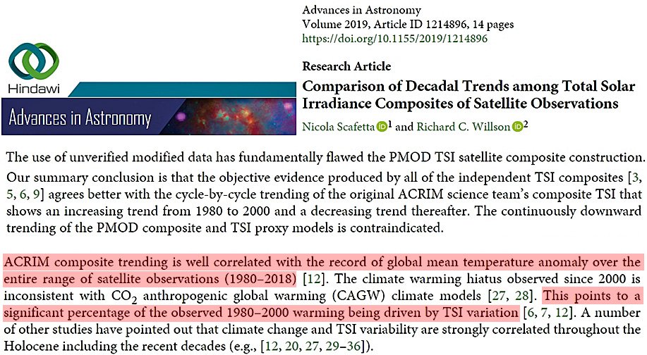
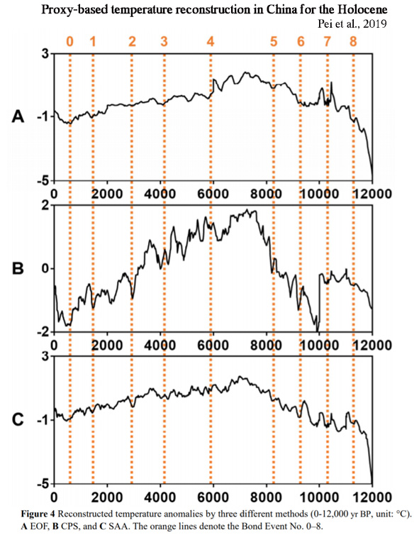
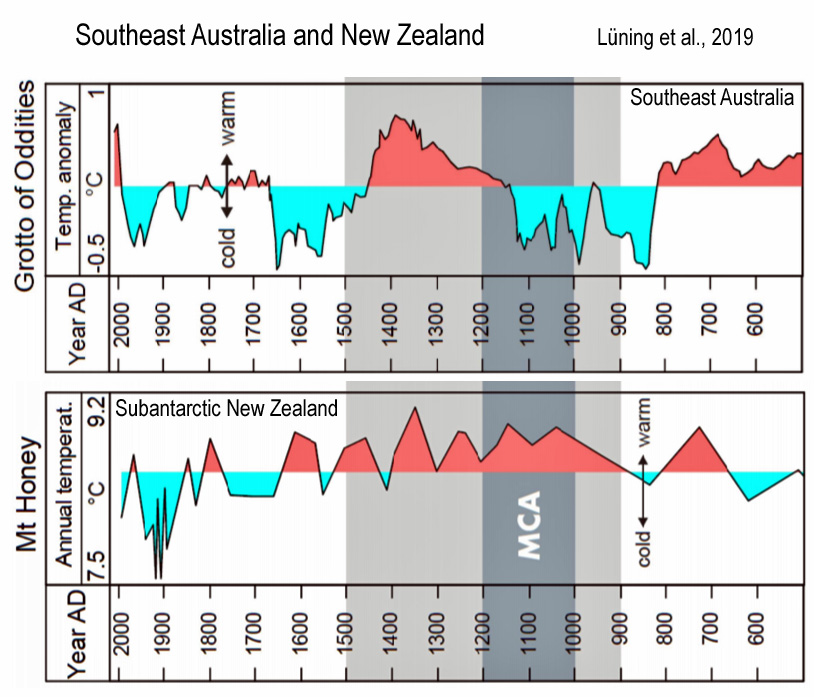
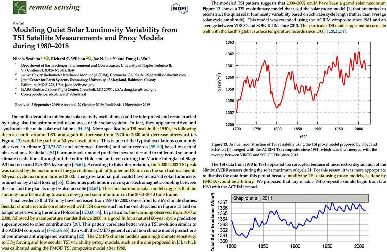
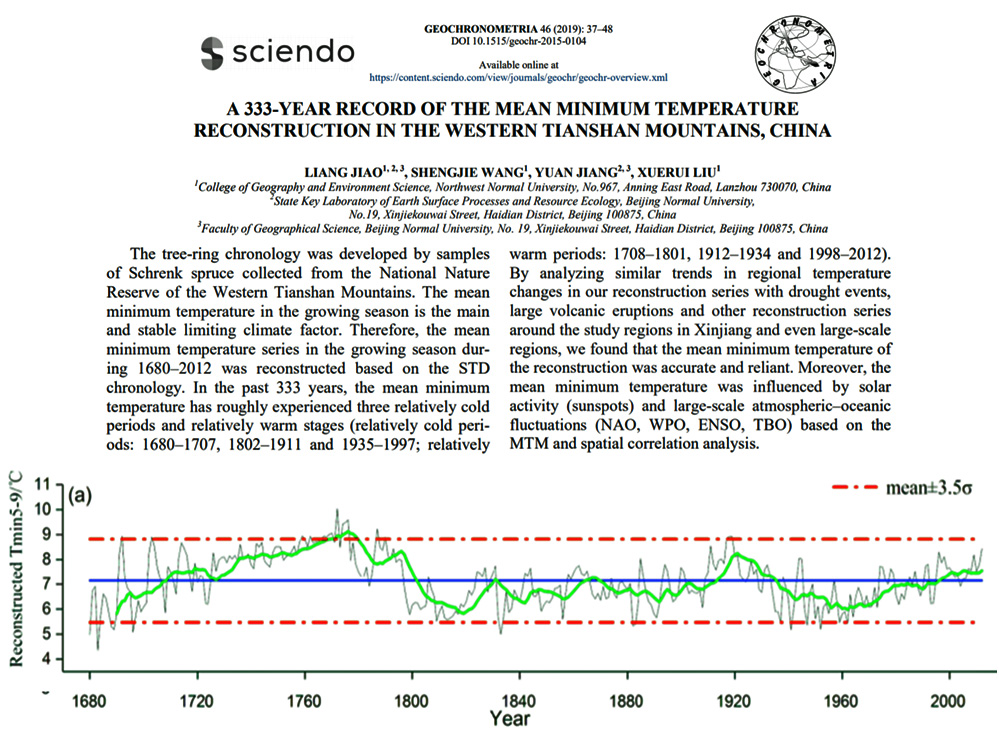
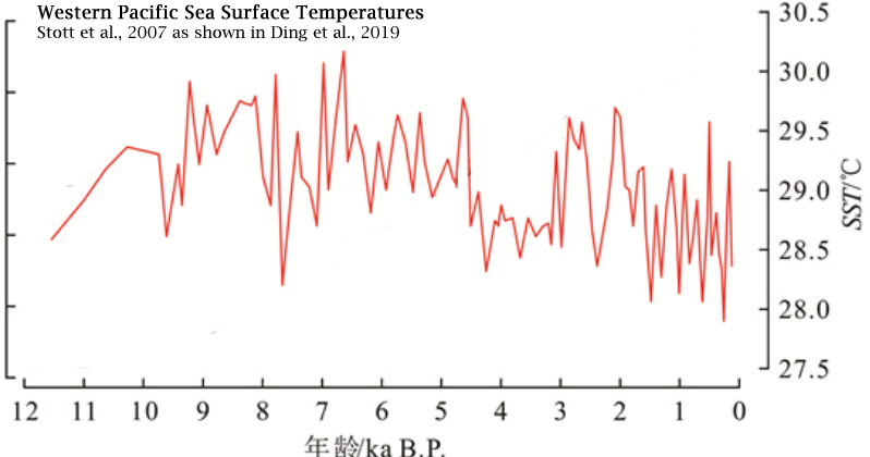
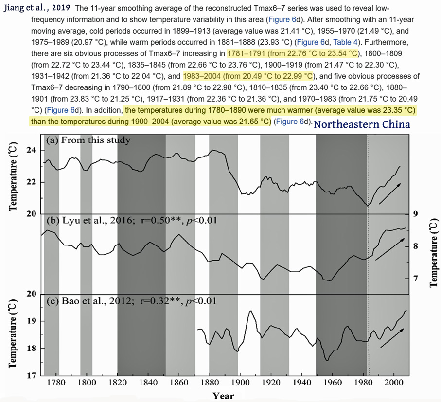
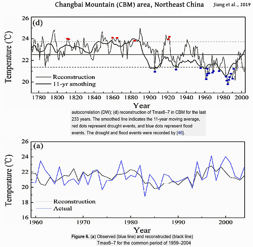
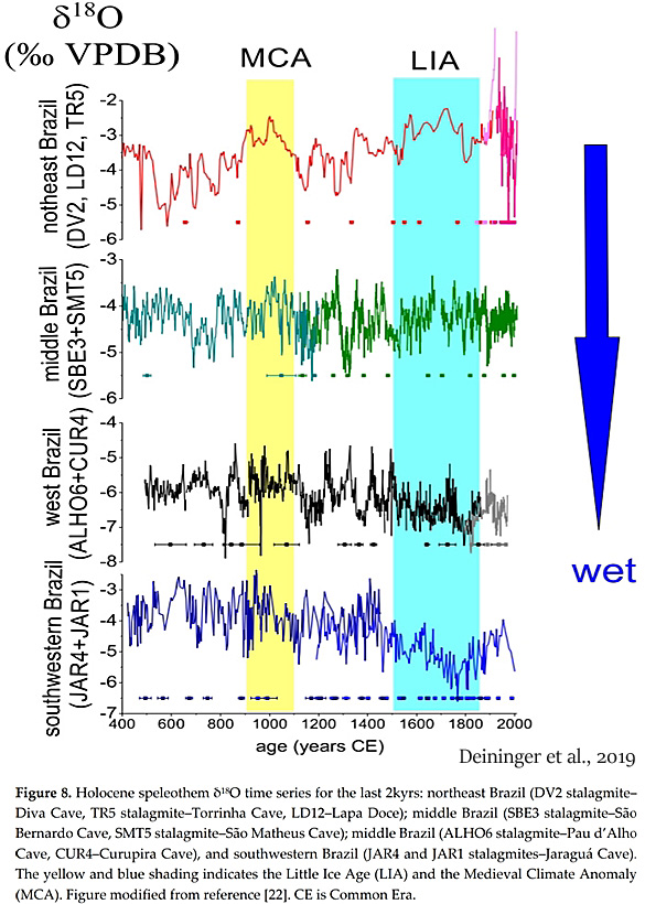
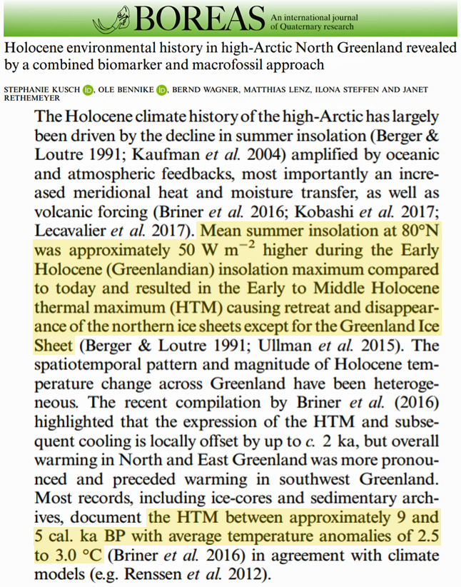
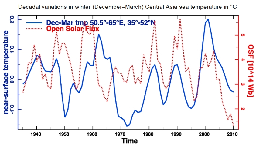
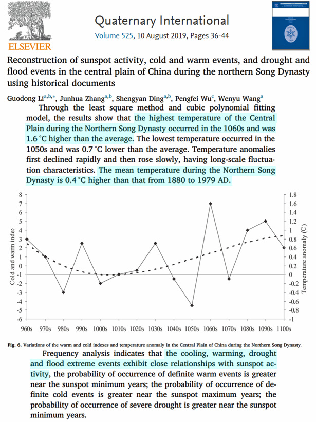
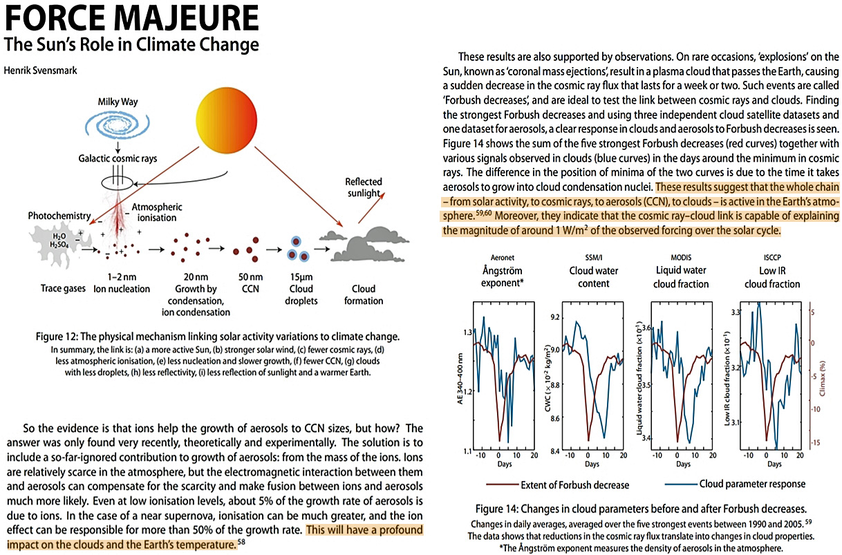
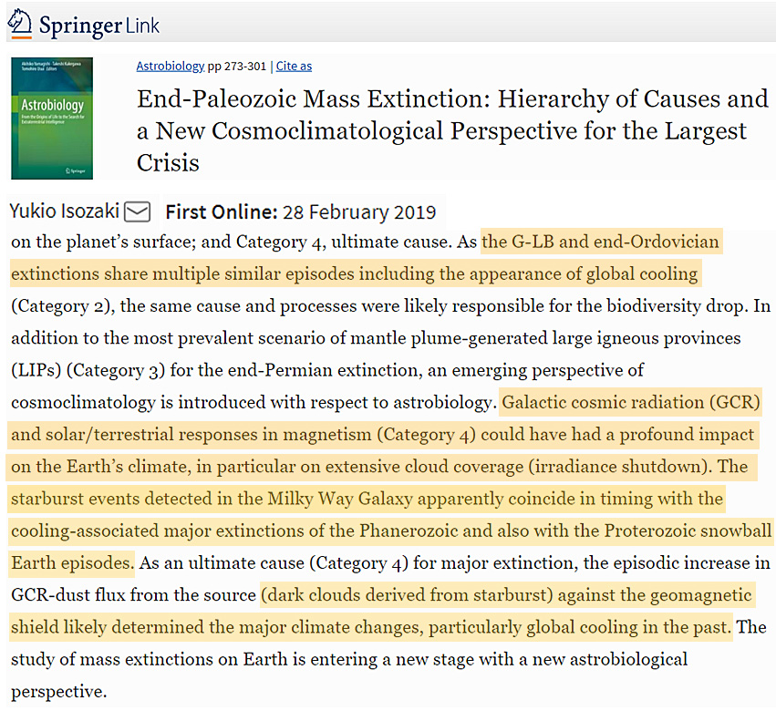
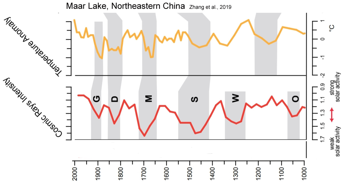
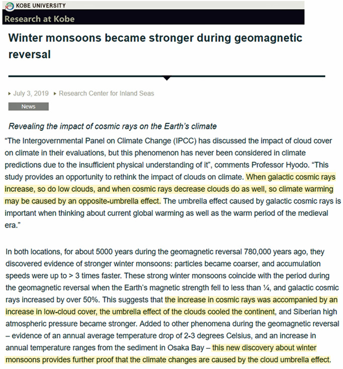
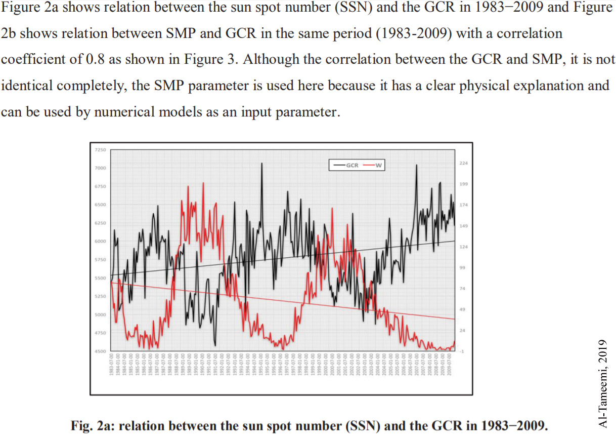
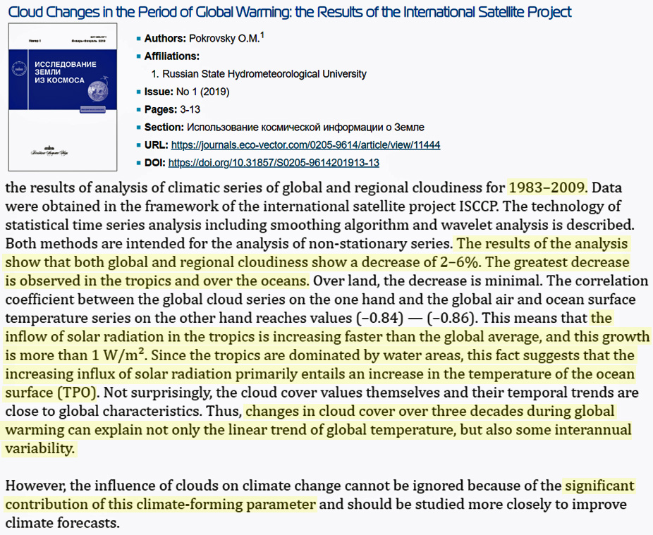
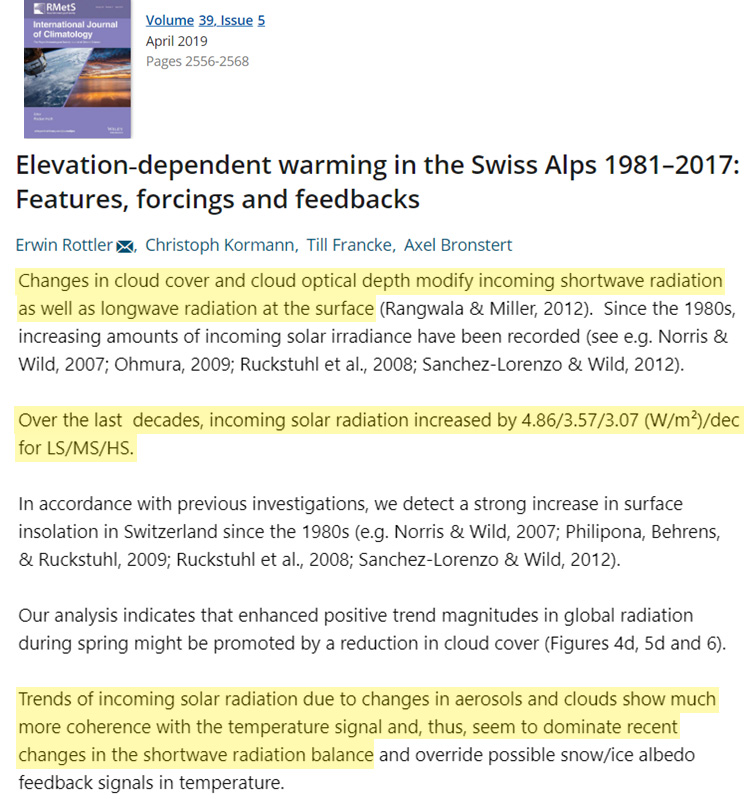
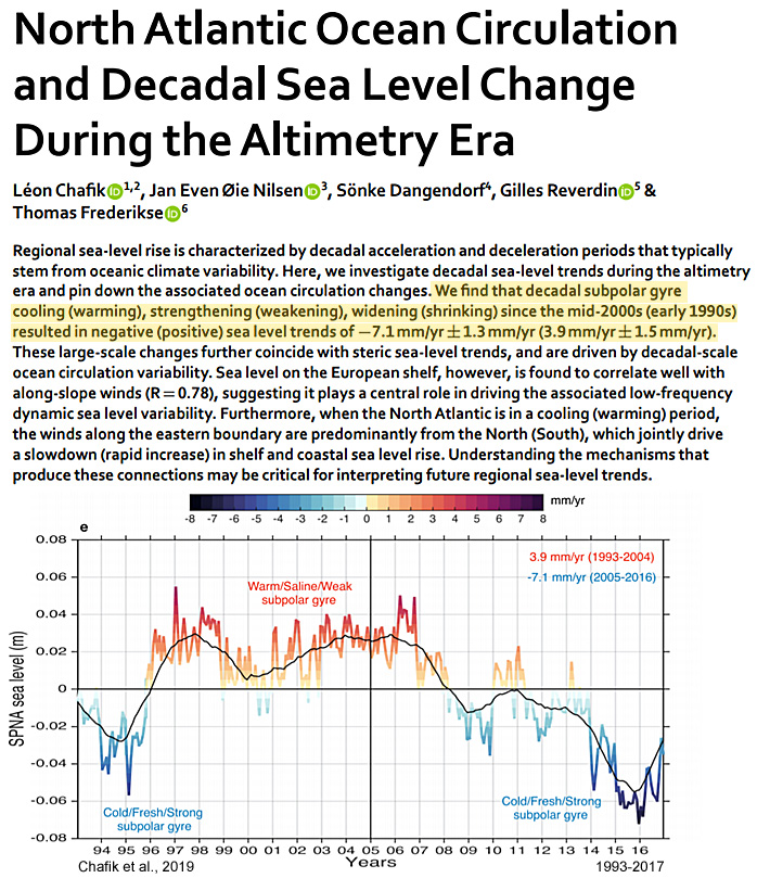
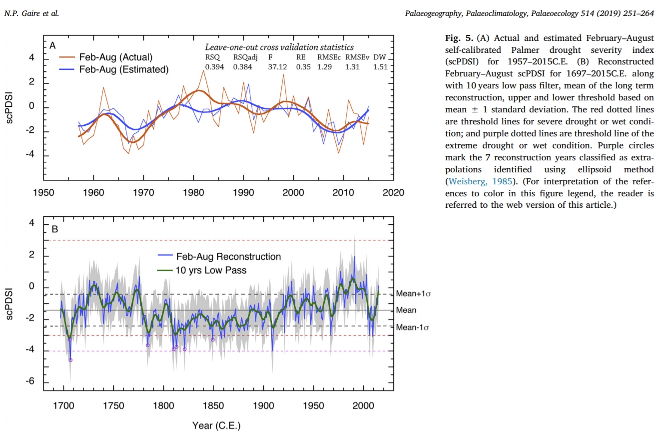
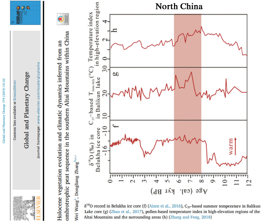
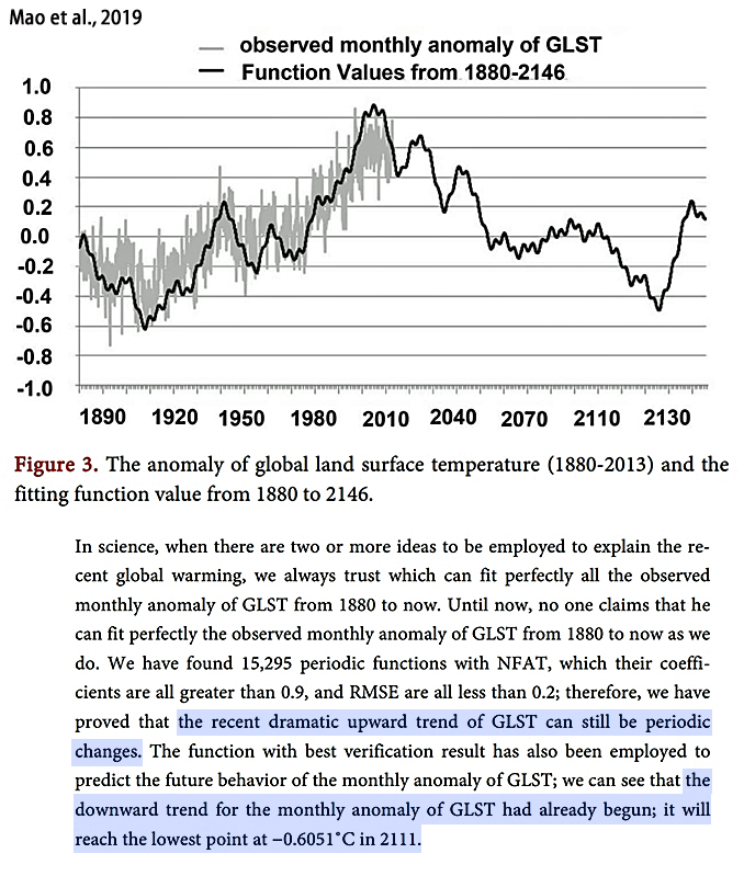
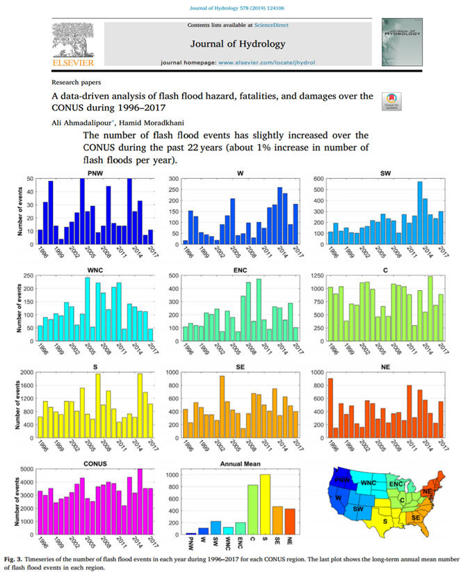
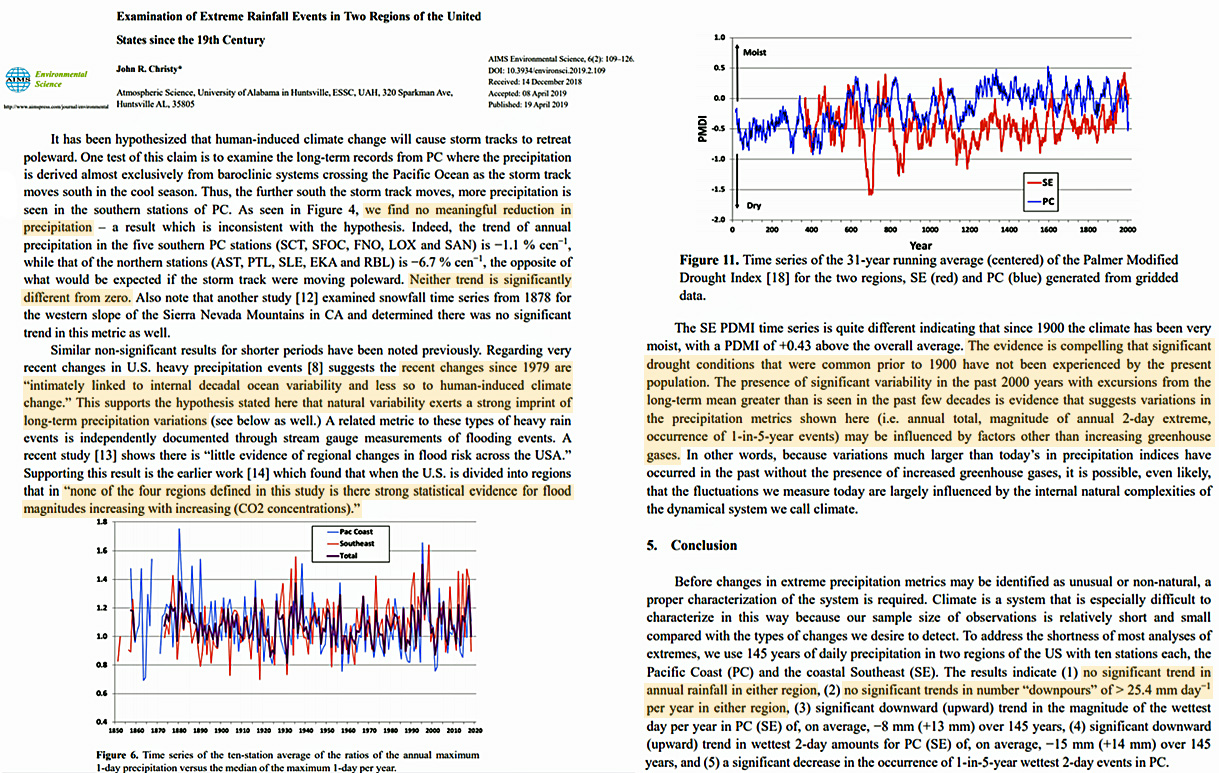
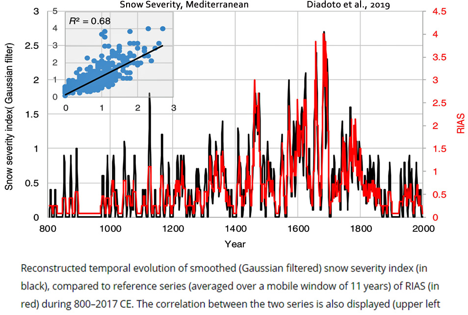
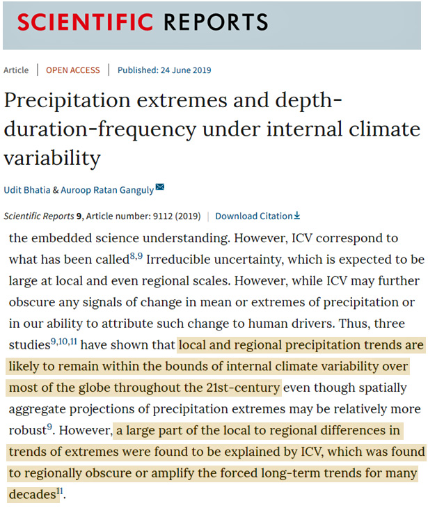
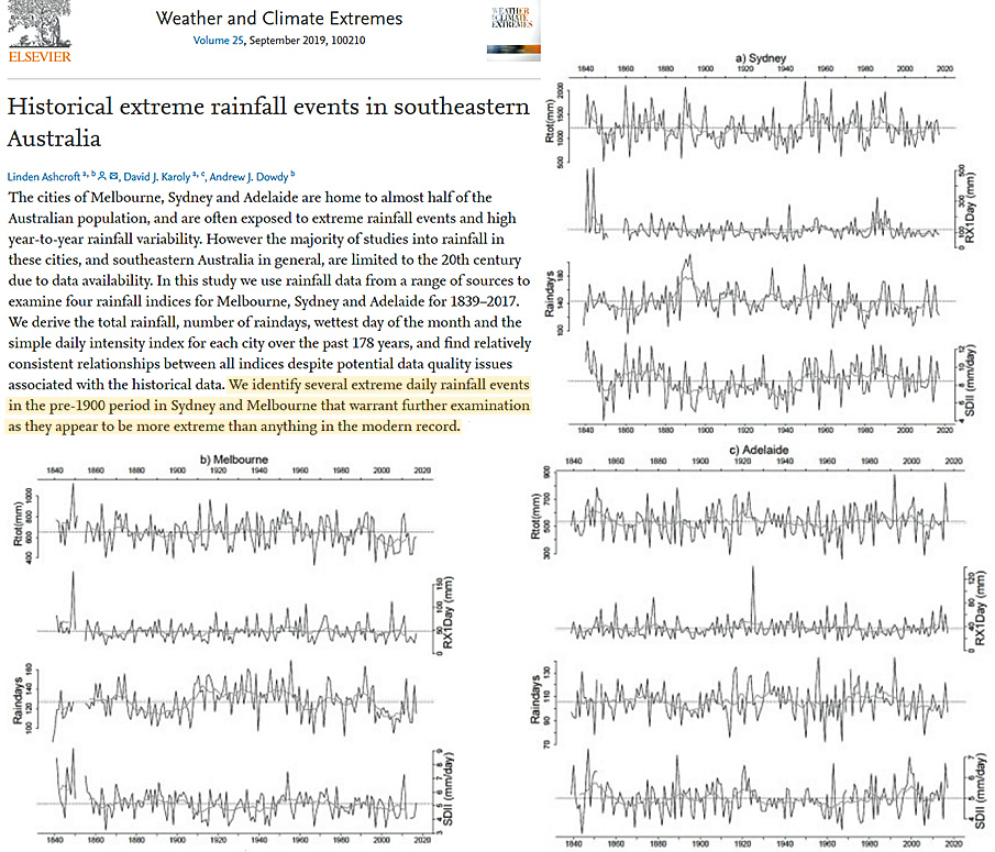
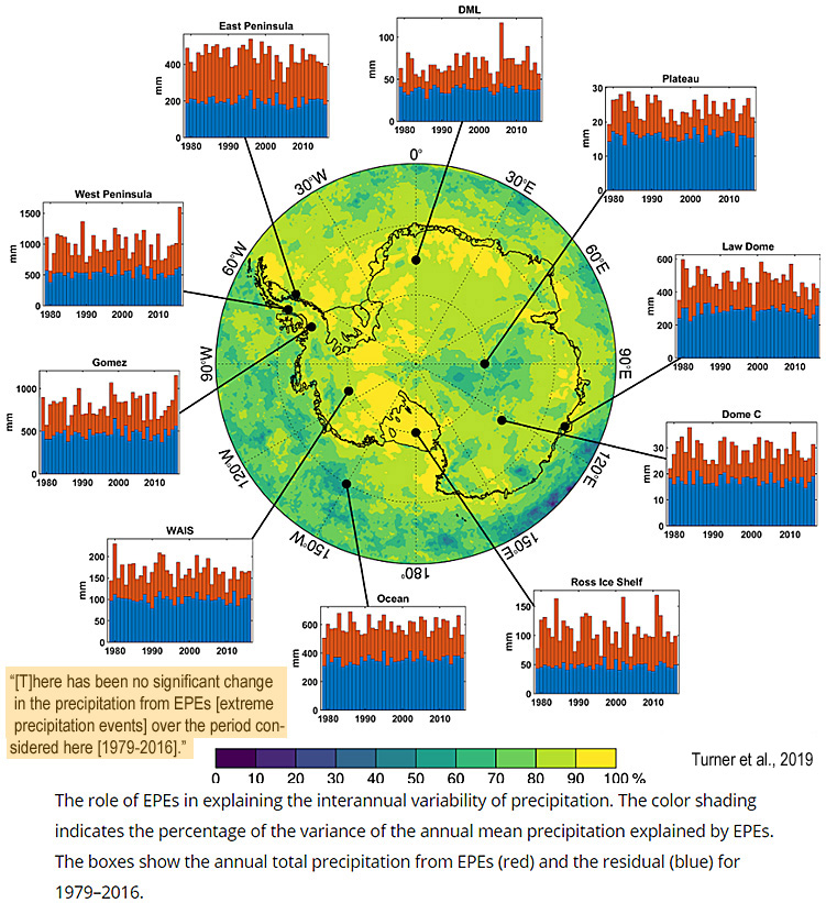
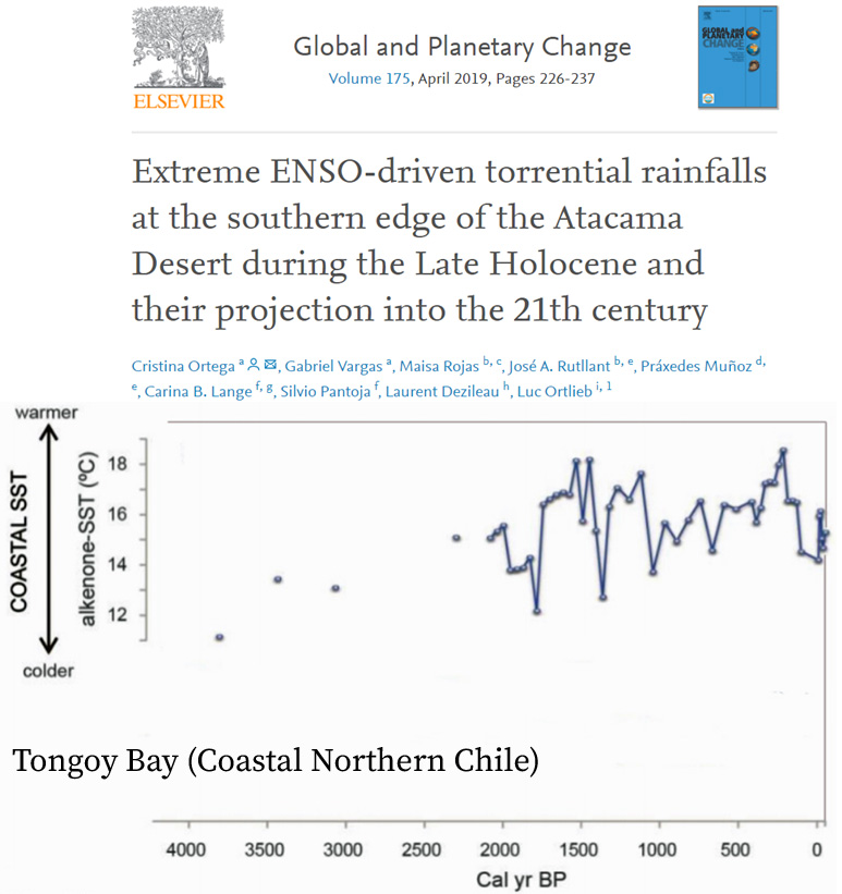
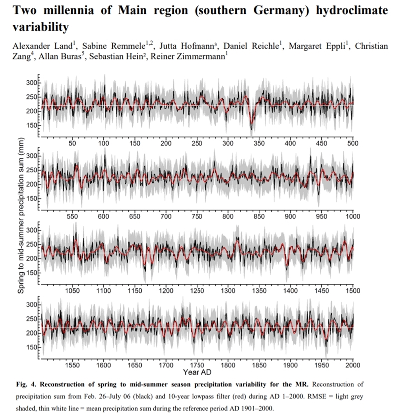
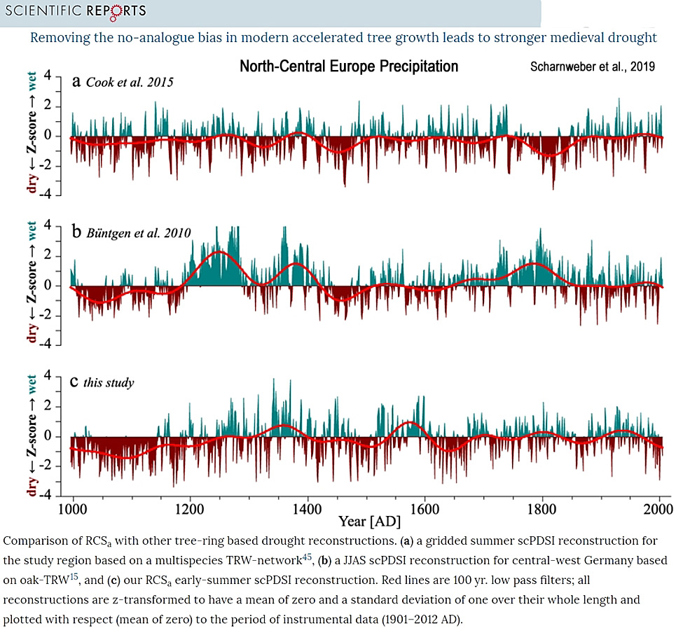
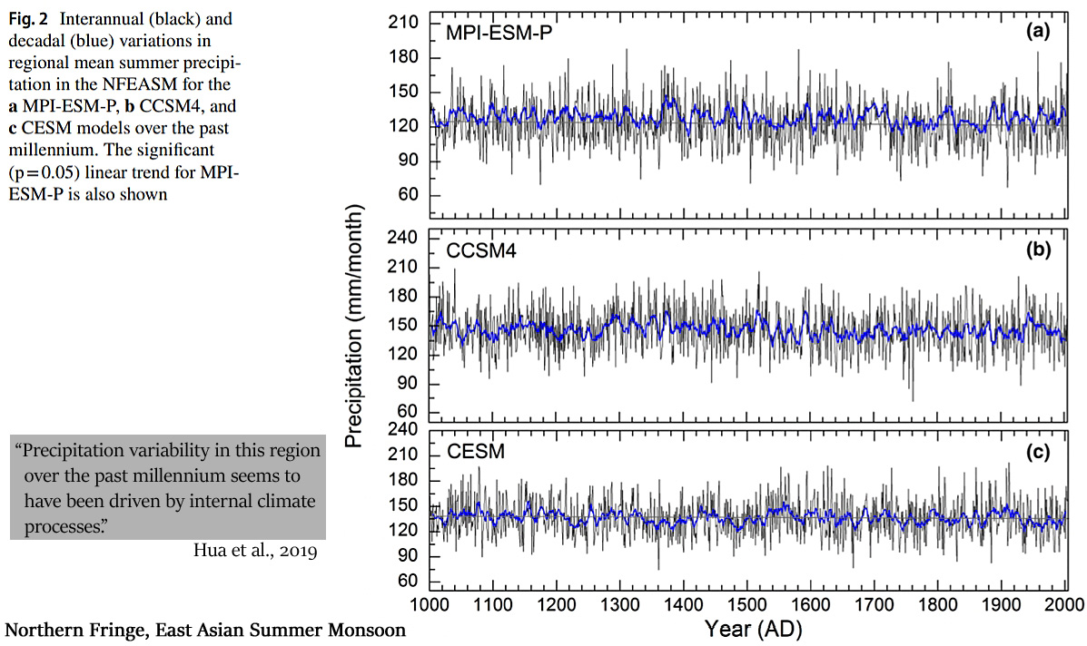
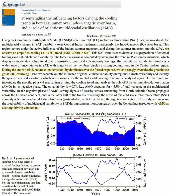
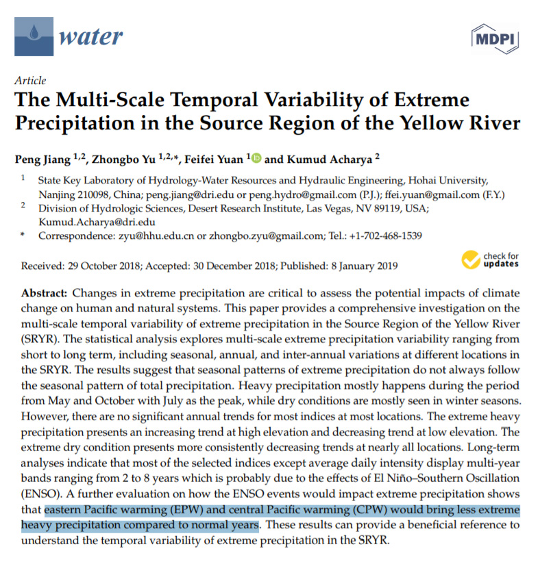
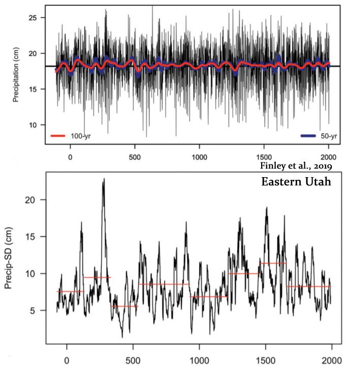
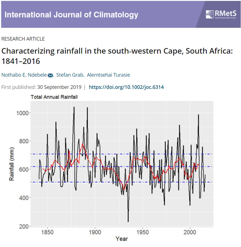
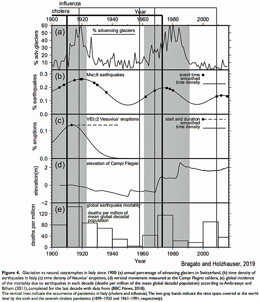
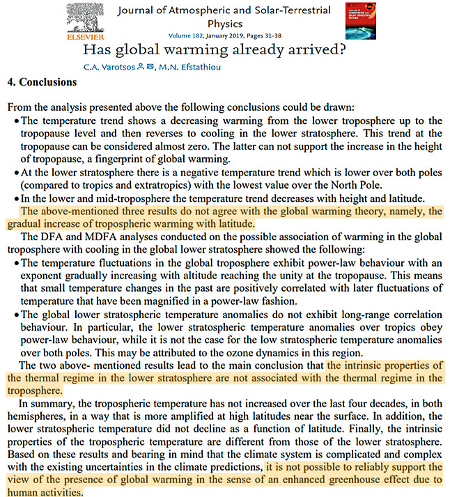
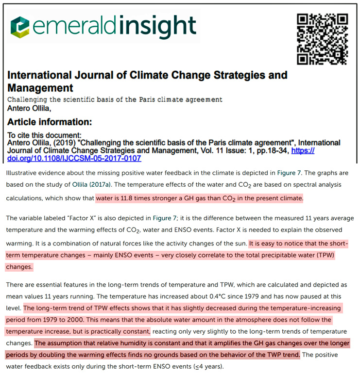
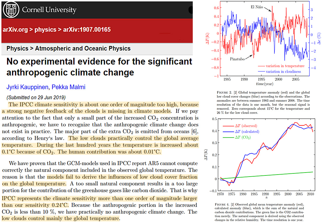
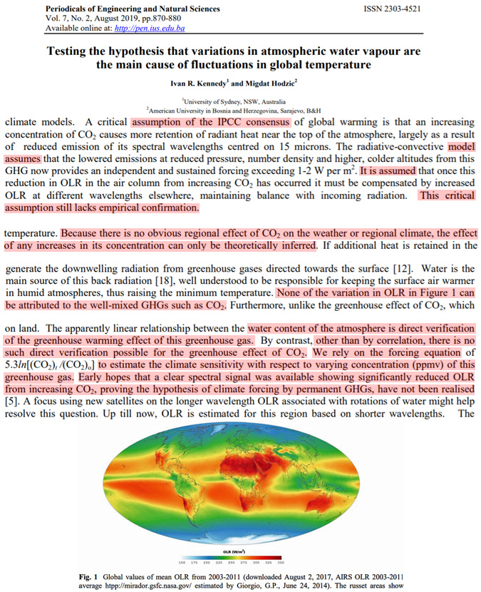
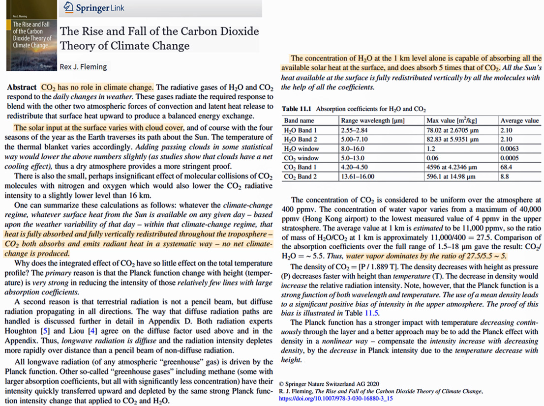
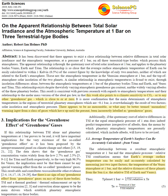
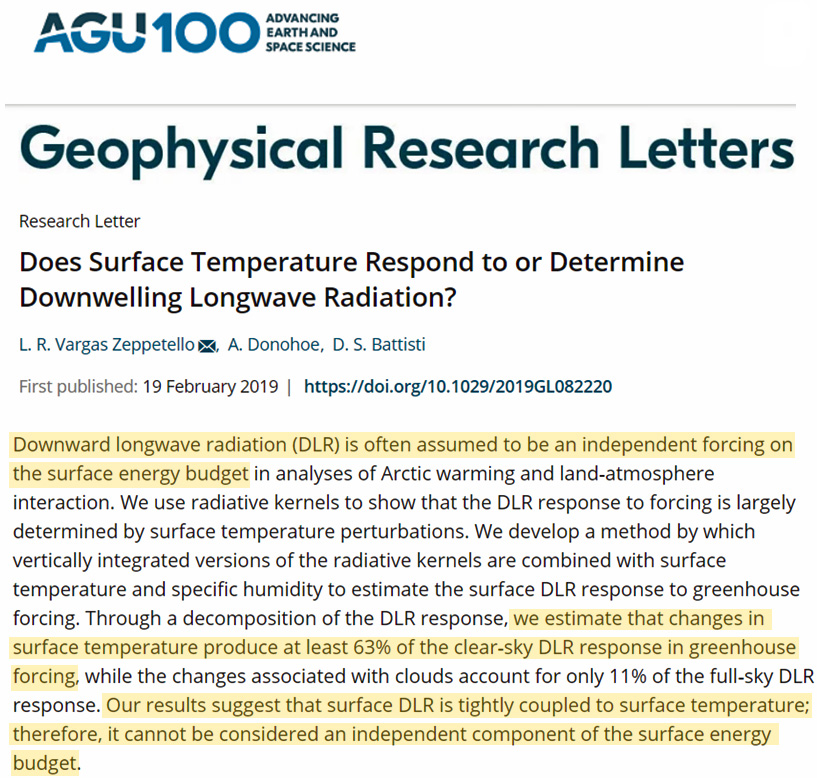
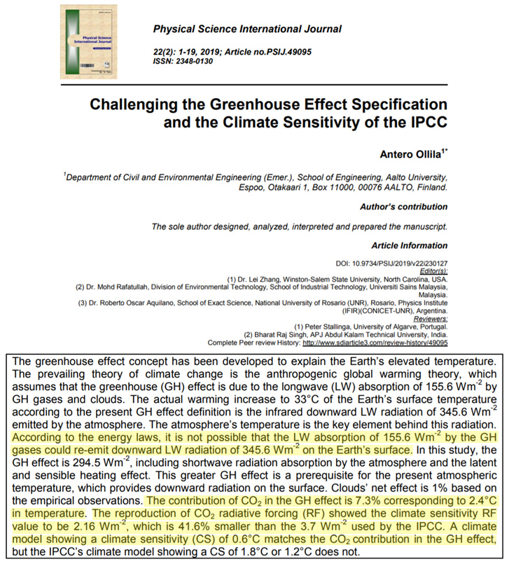
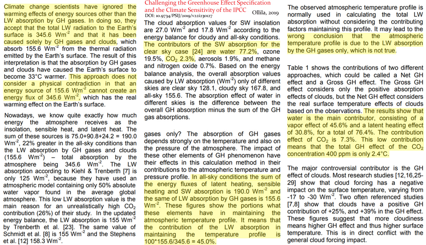


Recent Comments