By Frank Bosse and Fritz Vahrenholt
In February the sun was very quiet in activity. The observed sunspot number (SSN) was only 44.8, which is only 53% of the mean value for this month into the solar cycles – calculated from the previous systematic observations of the earlier cycles.
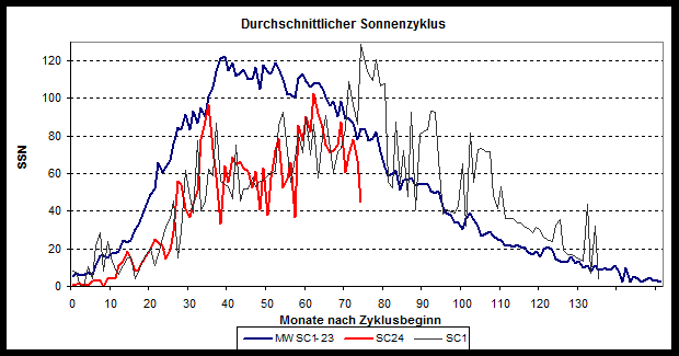
Figure 1: Solar activity of the current Cycle No. 24 in red, the mean value for all previously observed cycles is shown in blue, and the up to now similar Cycle No. 1 in black.
It has now been 75 months since cycle No. 24 began in December, 2008. Overall this cycle has been only 53% of the mean value in activity. About 22 years ago (in November 1992) Solar Cycle No. 22 was also in its 75th month, and back then solar activity was 139% of normal value. The current drop in solar activity is certainly quite impressive. This is clear when one compares all the previous cycles:
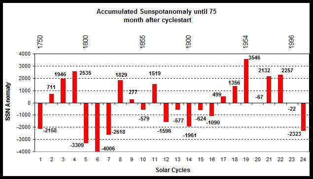
Figure 2: Comparison of all solar cycles. The plotted values are the differences of the accumulated monthly values from mean (blue in Figure 1).
The solar polar magnetic fields have become somewhat more pronounced compared to the month earlier (see our Figure 2 “Die Sonne im Januar 2015 und atlantische Prognosen“) and thus the sunspot maximum for the current cycle is definitely history. It’s highly probable that over the next years we will see a slow tapering off in sunspot activity. Weak cycles such as the current one often follow. Thus the next minimum, which is defined by the appearance of the first sunspots in the new cycle 25, may first occur after the year 2020. The magnetic field of its sunspots will then be opposite of what we are currently observing in cycle 24.
The radiative forcing of CMIP5 models cannot be validated?
A recent paper by Marotzke/ Forster (M/F) is in strong discussion here at climateaudit.org with more than 800 comments. Nicolas Lewis pointed out the question: Is the method of M/F for evaluating the trends infected by circularity?
There is not only a discussion about the methods, but also about the main conclusion: “The claim that climate models systematically overestimate the response to radiative forcing from increasing greenhouse gas concentrations therefore seems to be unfounded.”
Is the natural variability really suppressing our efforts to separate the better models of the CMIP5 ensemble from not so good ones?
Here I present a method to find an approach.
Step 1
I investigated the ability of the 42 “series” runs of “Willis model sheet” (Thanks to Willis Eschenbach for the work to bring 42 anonymous CMIP5 models in “series”!) to replicate the least square linear trends from 1900 to 2014 (annual global data, 2014 is the constant end-date of these running trends). I calculated for each year from 1900 to 1995 the differences between the HadCRUT4 (observed) trends ending in 2014 and the trends of every “series” also ending in 2014. The sum of the squared residuals for 1900 to 1995 the differences between the HadCRUT4 (observed) trends ending in 2014 and the trends of every “series” also ending in 2014.
The sum of the squared residuals for 1900 to 1995 for every “series”:
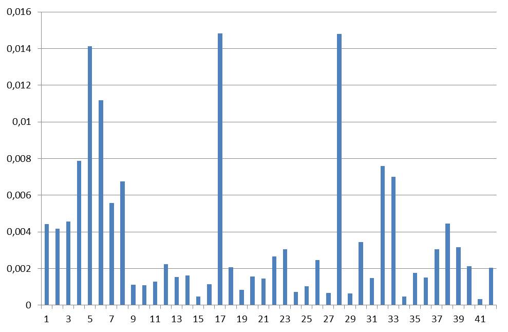
Figure 3: The sum of the squared residuals for the running trends with constant end in 2014 from 1900,1901 and so on up to 1995 for every “Series” in “Willis sheet”. On the x-axis: the series 1…42.
Step 2
We describe the same procedure described in Step 1, but this time with the trends up to 2004, only 10 years before the end of the trend series:
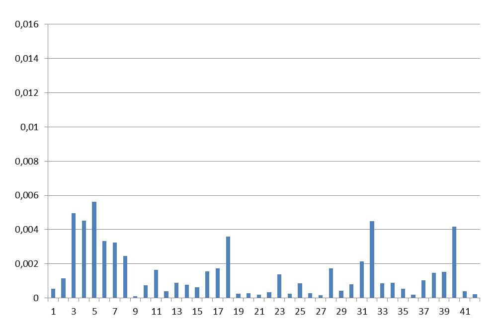
Figure 4: The sum of the squared residuals for the running trends with constant end in 2014 from 1900, 1901 and so on up to 1995 for every “series” in the “Willis sheet”. On the x-axis: the series 1…42. The ordinate scale is the same as in Figure 3.
Here one sees that the errors for the trends until 2004 on average are much smaller (Figure 4) than they are for the trends up to 2014 (Figure 3). That is no wonder as the parameters of most models for the time period up to 2005 were “set“. Thus the depiction of the trends of the models up to 2014 are also well in agreement with observations:
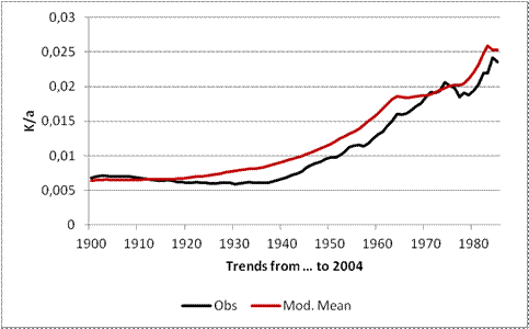
Figure 5: The trends of the model mean (Mod. Mean, red) in °C/ year since 1900, 1901 etc. up to 1985 with the constant end-year 2004 compared to observations (black).
Obviously the setting of the model parameters no longer “hold” as the errors up to the year 2014 rise rapidly.
Step 3
We calculate the quotients of the errors for the 2014 trends divided by the errors for the 2004 trends (See Figure 4) for every single series and make a 2-dimensional check:
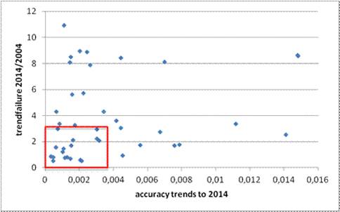
Figure 6: The single series as plotted points. The coordinates are determined by the trend error der until 2014 (X axis) and the ratio of the error up to 2014/2004 (Y axis). The red rectangle marks the “boundaries”, the “good“ series are inside, the “bad“ are outside.
The borders are represented by the standard deviations of both series.
The y-axis in Figure 6 above is the quotient of failures in trend estimations to 2014 (see Figure 5) divided by the trend estimations to 2004 (see Figure 4) with a standard deviation of 3.08; the x-axis is the accuracy of the series in trend estimation for the running trends with the constant end year 2014 (see Figure 5) with a standard deviation of 0.0038. The big differences of many series (up to a factor of 11) between the trend errors compared of 2004 and the trend errors to 2014 is impressive, isn’t it? The stability of the series with great differences seems to be in question, that’s why they are “bad”.
Step 4
Now comes the most interesting part: From the 42 runs of different series, I selected the “good” ones which are within the borders of the red rectangle in Figure 4 and calculated their average. The same procedure was done with all the “bad” ones.
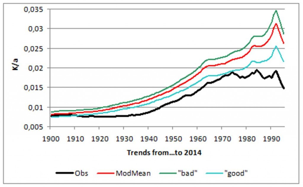
Figure 7: The selected “good” series (see step 1-3), the series mean of all 42 series, the “bad” ones and the observations for rolling trends with constant end-year 2014 in K per annum.
The “good” (blue) series produce a remarkably better approach to the observations than the model mean (red) and the “bad”( green) show the worst performance.
Up to this point we didn’t know what model was behind what “series” in the “Willis sheet”. Thanks to the help from Willis Eschenbach and Nic Lewis we just learned the assignment and the properties of the models behind the “series”, also their corresponding sensitivity with respect to forcing by GHG. The mean value of the transient climate response (TCR), which is the expression for the calculated greenhouse gas effect, is approximately 1.6 for the “good“ models, the model mean (all models) is 1.8 and the “bad” model mean is 1.96.
As one observes is Figure 7, the selection of the “good” models “improves” the convergence towards the observations. For this a TCR of approximately 1.3 is assumed, compare to our blog post “Wie empfindlich ist unser Klima gegenüber der Erwärmung durch Treibhausgase? (How sensitive is our climate with respect to warming from greenhouse gases)“.
Conclusion
The mean of the models overestimates the radiative forcings in the global temperature to 2014. The objectively better models have a lower mean of TCR. The “bad” models have a higher mean of TCR. Many models are perhaps “over tuned” for the trends to 2005. The result is a dramatic loss in forecasting quality beyond the tuning period. Are Marotzke and Forster wrong? Will we ever hear them admit it? There are reasons for doubt.



“Many models are perhaps “over tuned” for the trends to 2005.”
Overadaptation.
Climate scientists learn the pitfalls of modeling the hard way.
(Well, who believes in earnest they started out as ignorant as they pretend to be? I sure don’t. Just look at the loving relationship between the late Steve Schneider and TV cameras.)
Climate Change marries Socioeconomic Factors to create rapidly rising damages in river floods, reports the American-oligarch funded WRI.
German article:
http://www.n-tv.de/wissen/Flutschaeden-werden-sich-vervielfachen-article14640301.html
English : WRI got 40 million by oligarch in 2014 (et presto there’s the catastrophist news)
http://en.wikipedia.org/wiki/World_Resources_Institute
In presenting the CMIP5 dataset, Willis raised a question about which of the 42 models could be the best one. I put the issue this way: Does one of the CMIP5 models reproduce the temperature history convincingly enough that its projections should be taken seriously?
To reiterate, the models generate estimates of monthly global mean temperatures in degrees Kelvin backwards to 1861 and forwards to 2101, a period of 240 years. This comprises 145 years of history to 2005, and 95 years of projections from 2006 on-wards.
I identified the models that produced an historical trend nearly 0.5K/century over the 145 year period, and those whose trend from 1861 to 2014 was in the same range. Then I looked to see which of the subset could match the UAH trend 1979 to 2014.
Out of these comparisons I am impressed most by the model producing Series 31, which Willis confirms is output from the inmcm4 model.
It shows warming 0.52K/century from 1861 to 2014, with a plateau from 2006 to 2014, and 0.91K/century from 1979-2014. It projects 1.0K/century from 2006 to 2035 and 1.35K/century from now to 2101.
Note that this model closely matches HADCrut4 over 60 year periods, but shows variances over 30 year periods. That is, shorter periods of warming in HADCrut4 run less warm in the model, and shorter periods of cooling in HADCrut4 run flat or slightly warming in the model. Over 60 years the differences offset.
In contrast with Series 31, the other 41 models typically match the historical warming rate of 0.05C by accelerating warming from 1976 onward and projecting it into the future.
Over the entire time series, the average model has a warming trend of 1.26C per century. This compares to UAH global trend of 1.38C, measured by satellites since 1979.
However, the average model over the same period as UAH shows a rate of +2.15C/cent. Moreover, for the 30 years from 2006 to 2035, the warming rate is projected at 2.28C. These estimates are in contrast to the 145 years of history in the models, where the trend shows as 0.41C per century.
Clearly, the CMIP5 models are programmed for the future to warm more than 5 times the rate as the past.
I forgot to provide the period trends for inmcm4
The best of the 42 models according to the tests I applied was Series 31. Here it is compared to HADCRUT4, showing decadal rates in degrees C periods defined by generally accepted change points.
Periods HADCRUT4 SERIES 31 31 MINUS HADCRUT4
1850-1878 0.035 0.036 0.001
1878-1915 -0.052 -0.011 0.041
1915-1944 0.143 0.099 -0.044
1944-1976 -0.040 0.056 0.096
1976-1998 0.194 0.098 -0.096
1998-2013 0.053 0.125 0.072
1850-2014 0.049 0.052 0.003
Ron C,
in other words the model has all this wonderful physics and is still basically “tuned” for a trend.
This article investigates none of the actual climate features such as precipitation, wind, clouds, ice…
KuhnKat, the inmcm4 model is described in a recent paper, Tolstykh et al, 2014.
They did forecasts for 1989-2010, and claim some skill in representing the 1998 El Nino. Of course, none of these models can deal with sub-grid phenomena. At least this one approximates reality, as we know it from flawed temperature datasets.
The paper can be downloaded here:http://www.researchgate.net/profile/Anatoly_Gusev2
This method is horrible.
If you want to compare models to reality, you have to factor in, that there are differences between the assumptions made for the models and reality, which do NOT alter the major result of the model.
perhaps the most typical example of a model is a crash test dummy.
It does not look lkike me and most likely< not liek you either. So we should get rid of them?
Now it turns out, that the population is changing and the crash test dummy do no longer representing obese people well.
http://www.washingtonpost.com/blogs/wonkblog/wp/2014/10/28/a-depressing-sign-of-americas-obesity-problem-fatter-crash-test-dummies/
So the model has to be adjusted, but that does not make it bad.
Again: This analysis is simplicistic and basically useless.
sod, comparing models used in the car industry to climate models is rather unfair to the kids in climate science. Because, the climate science kids don’t validate their models.
NOTHING in safety critical development happens without validation. IT CANNOT BE USED WITHOUT VALIDATION.
Try working in safety critical development. I do.
It shows just how ignorant this S.O.B is !
Car industry models have been validated time and time a and time again. If they didn’t work, cars wouldn’t work.
no climate model has EVER been validated.
In fact, all REAL data invalidates them !!
In the beginning I was looking for papers validating climate model sourcecodes. I was flabbergasted by not finding any. Then I understood that they have NO quality control AT ALL.
I worked with FORTRAN code written by professors in non-computer science domains, in various projects (the task was invariably to somehow translate the geniuses work into a product).
Let’s just say, their code generally does not look like it’s ever been real life tested. Marginal error recovery if at all, interfaces unusable to the subgenius, etc.
The source code of most climate models is a mess. As you say; no source code control at all. No configuration control. That means that, unless somebody has taken an “image” of the source tree, that the results aren’t reproducible.
The source code base is a swill.
There was, in the source code I’ve looked at in two classes of “models”, no checking of the plausibility of input data. Hence, the interpretation of the “NO DATA” magic number (grrrrrrrrrr) when mis-typed as reasonable data and inevitable inclusion as a starting point for a projection.
The presently-used models are based on expanding what seems to be FORTRAN II code (ca. 1970) with very coarse GCM’s based on 5×5 grids. The thermodynamics break down on the more-trapezoidal to triangular grid cells near the polar regions because the geometry is unaccounted for in at least one of the models I took a look at.
It doesn’t get much better when the granularity is reduced because the algorithms don’t change to correct that problem. Array sizes grow and more fudge factors appear.
AFAICT; the GCM’s “knew” nothing about dawn and dusk. TSI was taken as a constant. As was albedo. That’s the depth of modelling one could expect from an undergraduate student in Physics/Thermodynamics/Fluid Mechanics.
There are far too many arbitrary fudge factors and Finagle constants in the models to make them work.
“which do NOT alter the major result of the model”
Precisely, sob !!
Drop the CO2 demonisation, and the models have a far better chance of meeting reality !!!
Also, they need to stop hind-casting an adjusting their “variables” to fit to the junk that is GISS/HadCrud….. no wonder they can’t get any where near reality !! DOH !!!
Yes.. you are a crash test DUMMY !!
And very simplistic
but not completely useless.. you show the moronity of the average alarmista apostle.
“This method is horrible.”
If you don’t understand because of your base ignorance, just say so.. !!