CO2 or Ocean Cycles?
By Ed Caryl
We are all aware (or should be) of the warming that took place from the 1970’s to the 1990’s. The calamitologists are firmly convinced that this rise in temperature was due to rising CO2 in the same period. The lukewarmists think it was a combination of factors that perhaps contain some warming due to CO2. Then there is another group who think it was all due to the sun or ocean cycles.
This article will compare an ocean cycle, the Atlantic Multi-decadel Oscillation (AMO), and CO2 as temperature drivers over the last 133 years, since 1880. The annual temperature data is from GISS. The plots are scatter diagrams with temperature on the vertical axis and AMO index or CO2 atmospheric concentration on the horizontal axis.
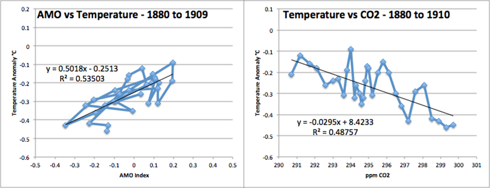
Figures 1a and b are XY plots of temperature vs. AMO (1a) and temperature vs. CO2 (1b).
The period of 1880 to 1910 was a period of cooling. Unless CO2 was driving that cooling, it seems clear that ocean cycles (or some third forcing, such as solar) were responsible.
Figures 2a and b are XY plots of temperature vs. AMO (2a) and temperature vs. CO2 (2b).
The period from 1911 to 1936 was one of warming, on a similar scale to the recent warming. The amount of CO2 increase has been thought not to be responsible for the warming, and attributed to ocean cycles. Climate sensitivity is easy to calculate from the slope of the trend lines in the temperature versus CO2 plots. Simply multiply the “x” value by the minimum CO2 concentration. If the warming in this period was totally due to CO2, the associated climate sensitivity would be 8.3°C for CO2 doubling from 300 ppm, a value that all will agree is much too large. Again, CO2 isn’t providing the warming.
Figures 3a is a plot of temperature vs AMO and 3b a polot of temperature vs CO2.
Figure 3c below is a zoom in on 1937 to 1950, the near vertical line at the left in figure 3b where CO2 actually reversed slightly for a time:
This was a period of cooling, and it is obvious that CO2 had nothing to do with it. Climate sensitivity would have been a negative 0.465°C for CO2 doubling from 310 ppm. During the cooling 1937 to 1950 period, sensitivity would have to have been an astounding negative 82°C for CO2 doubling. Again, ocean cycles or some other forcing were responsible.
Figures 4a and b are XY plots of temperature vs AMO (4a) and temperature vs. CO2 (4b).
The years from 1970 to 2000 were warming years as can be seen on both plots. Note the R2 values for both plots. Was the warming due to CO2? Or was it ocean cycles? The R2 values are voting for ocean cycles, but it isn’t definitive. Remember that Salby and myself have made cases for temperature driving CO2, and not the other way around. The slope of the CO2 trend in this period (climate sensitivity) is 3.64°C for CO2 doubling. This is the only time period where the putative climate sensitivity is reasonable, and close to the theoretical IPCC approved number.
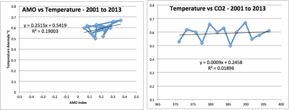
Figures 5a and b are XY plots of temperature vs. AMO (5a) and temperature vs. CO2 (5b).
Above is the recent past; the pause period. Not much is happening. The warming is so slight, that the computed climate sensitivity is 0.33°C for CO2 doubling from 370 ppm. The R2 value for CO2 is so low that it should be clear that something else besides CO2 is in charge. The slope on this AMO plot is positive, as it has been for all of the AMO vs temperature plots, but the points are clustered tightly and the R2 value is only 0.19.
In the 133 years since 1880, all the “CO2 is causing catastrophe” furor is based on one 30 year period in that long span. The remaining 103 years, where CO2 was obviously having no effect, are ignored, …are unexplained. Is this justified? Shouldn’t some effort be made to determine what has really happened? If CO2 is the driver of warming periods, and ocean cycles are driving cooling periods, then climate sensitivity was 8.3°C in the early 20th Century, 3.64°C in the late 20th Century, and 0.33°C now. If CO2 is assumed responsible for half the warming, as the IPCC suggests, and other greenhouse gases are responsible for the rest, the numbers then are: 4.15°C for the early 20th Century, 1.82°C for the late 20th Century, and 0.165°C for the last decade. This may be another indication that climate sensitivity has hit a low limit.
The numbers for CO2 become even lower if changes in solar radiation, solar magnetic effects, cosmic rays, aerosols, volcanic sulfate, soot, dust, water vapor, and changing cloud cover are thrown into the forcing mix. The problem is lack of data. We have good data from satellites only for the last 34 years for temperature, and less than that for many of these other factors. On this paucity of data we are betting our economic future on all kinds of ill-thought out “renewable solutions” that in the long run we will regret.


The 1910 to 1940 similar rate of warming to the late 20th century has been a thorn in their side for years. The subsequent cooling in the face of ever rising co2 is simply speculated away.
You often hear about how the rate of recent warming is unprecedented. Let’s look at a 60 year period from the past. We know that co2 rise follows temperature rise.
Source for AMO and CO2?
AMO from here:
http://www.esrl.noaa.gov/psd/data/timeseries/AMO/
CO2 is a combination of the Law Dome ice core series and the Keeling CO2 from Mauna Loa.
Ed – Unfortunately I have to pull you up on this one.
The AMO is detrended NH Atlantic SST’s. Therefore it isn’t independent of global temperature and graphing these two variables against each other is of very questionable value.
The point you make is absolutely correct, just the methodology is not a good one.
My approach is always to link graphs of the AMO, PDO and HadCRUT 3v with a sinusoidal regression line, or something similar (like detrended HadCRUT 3v here).
That way you can see the amplitude of the oscillation, and the correspondence of the trough with the IPCC’s century start year (1906) and the peak in the cycle corresponding to the IPCC’s end year 2005. Therefore removing the peak-trough temperature swing is both justified and necessary. It was worth nearly 40% of the temperature “rise” last century and is a complete artefact.
The oscillation is persistent as Knight et al 2005 (GRL) finds over a period of at least 1400 years. Therefore it cannot be related to mankind’s actions.
I know all that. AMO is not independent, nor is PDO. But that is part of the point, what we are seeing in global surface temperature is ocean temperature cycles. The next question is, what is driving those cycles? Are those cycles resonances? The atmosphere is not resonant, the Q is too low. But it is, I think, just possible that the ocean basins, or some combination of currents, might resonate. We know, for instance that the ENSO is somewhat regular. Perhaps that makes something in the Atlantic “ring” at the lower frequency. I’m speculating. The energy that sets these cycles into oscillation comes from somewhere. Ultimately, it comes from the sun’s oscillations. But what is/are the coupling mechanism or mechanisms?
The paper Knight et al 2005 links it to the thermohaline cycle which is plausible to me as a chemist (btw note who the last author is…seems to have ditched reality since he contributed to that paper!).
I am also struck by the close integer ratio to the solar cycle 62:10.66 = 6:1. It would be no surprise to me that a pumped resonance as a result of the configuration of the ocean basins is the cause. Especially since the AMO and PDO appear to have the same period but are a quarter cycle out of synch.
The cycle seems to be quasiperiodic, which probably also fits with the variability of the solar cycle.
But the bottom line is it was responsible for about 0.28 out of 0.74 C temperature rise last century and is not included in the IPCC ensemble models. It should be. But if they did they’d immediately drop their derived ECS by nearly 40%. CO2 and temperature may not correlate but I suspect calculated ECS values and government climate science budgets do.
Yes, it could be a high Q resonance of perhaps the ocean basins being excited by random inputs. Or, a resonance of other origin.
Here is one possibility. The Earth’s rotation axis is nutatiing with a period of about 18.6 years. However, that is only part of the story. In actual fact, the nutation takes the form of an elliptical cone, as shown here. The distance between the J2000 polar axis and the actual rotation axis looks like this. Its period is necessarily halved, to about 9.3 years.
Thus, the magnitude of the component of the magnetic moment of the Sun along the Earth’s rotation axis should have periods of about
T1 = 11*9.3/(11+9.3) = 5 years
T2 = 11*9.3/(11-9.3) = 60 years
Coincidence? Maybe. But, is there not a 5-ish year quasi-periodicity to the major temperature sets? Hard to say for sure, but there surely are several ups and downs which are in the neighborhood of 5 years.
Here is the spectrum:
http://www.pnas.org/content/94/16/8321.full.pdf
Kind of demonstrates why I am not partial to MEM type spectral analysis – tends to break up energy masses into spectral lines which may, or may not, provide insight into the actual process.
A quick FFT-based PSD analysis of my own shows energy generally centered around a little less than equivalent 5 year periodicity. What does that mean? Can we come up with reasonable variations in the parameters to give us ~3-5 years and 60-70 years?
Maybe. I need to chew on it some more…
It is always good to remember that when more than one variable correlates with something else (possibly causative) it is proof of NONE.
Ed: if you have two quasi-random variables, you should better use correlation in stead of regression. The CO2 level on the x-axis looks like a simple function of time. Are the values means over certain periods? With regression, the assumption is that they are fixed. Why should you break up the computation of correlation in time segments? So what is the correlation between temperature and CO2 level over the whole period? R2Dtoo: yes, all variables correlating with time correlate with each other. Probably, the mean income of households in the Netherlands correlates positively with CO2 level.
The values are annual means.
I broke the periods into warming and cooling periods. I also noticed that, when I plotted the whole 133 years (not shown), the xy plot points had a pattern where these periods were in different areas of the plot. I confess that I used that pattern to select the dividing years.
The CO2 level looks like a simple function of time because it has been steadily increasing over time, except in the 1937 to 1950 period. I think that during WWII the level was probably increasing then decreasing, but the ice core data doesn’t resolve that.
As you have probably guessed, I’m not a statistician.
I think the ice core data are questionable, frankly. Any time a derived measurement is presented for which there is no capability of closed loop test of the system response – inject input, observe output – I believe one must treat it with extreme caution.
Other measures, e.g., leaf stomata, give different results. It seems to come down to a vote on what most people think is the more reasonable result. But, that is a subjective process. Do we largely accept the ice cores because they show what most expect to see? That is a rather circular justification.
I agree. At the least, ice core data has very poor temporal resolution, that gets worse over time as the CO2 diffuses through the ice. Ice crystals grow over time and the crystal boundaries sweep bubbles ahead of the growth. In Greenland I once saw a display of ice crystals from several hundred feet down in the ice cap that were over an inch across. They were displayed like mineral crystals between polarizing filters. You could see that the crystal boundaries had swept up impurities. But I have never seen this described in the literature.
Ed, the problem you have is one of “signal to noise” ratios. The CO2 effect is expected to be persistent but is actually pretty small short-term compared with the natural cyclic things going on.
On the shorter time scale (1 to 2 decades) it is well known that other factors can predominate. Here are some examples drawn from the Lean and Rind breakdown of temperatures over a 30 year period shown on the following graph :
http://www.wright.edu/~guy.vandegrift/climateblog/smallfiles01/100218aipRindLeanTemp.jpg
The 30 year temperature trends are around 0.15 to 0.19 deg C per decade depending on which of the RSS, UAH, GISTEMP or C&W temperature data sets you take. From the Lean & Rind graphs then the natural random and/or cyclic effects have a peak to trough amplitude of :
– TSI (Total Solar Irradiance) = 0.1 deg C
– ENSO (El Nino Southern Oscillation) = 0.3 deg C
– Volcanoes causing cooling at random times = 0.25 deg C
Hence if you only do regression over a maximum of 15 years there is no way that the CO2 greenhouse effect is going to register compared with the random and cyclic natural things going on, and if they were all working to cause cooling at a particular point then they could produce an effect of more than 0.6 degrees cooling which would take the CO2 40 years to counteract!
So the thesis you have to prove or disprove is not that “increases in CO2 cause temperature increases over a period of 1-2 decades”, but more that “increases in CO2 cause temperature increases over a period of 3 decades or more”.
So it would be more valuable to do correlations based on 30 years or more, at which point the IPCC expectation would be for CO2 to give a reasonable correlation, or you could do a multiple regression against all four possible causes at once to get a regression equation of Temp = a x TSI index + b x ENSO index + c x volcano index + d x CO2 change, or you can add any other index you like to the mix. But even so you would probably have to use a long period to get meaningful results.
In any event no-one in their right mind is saying it is CO2 or natural variation index XYZ. It should be CO2 and natural variation XYZ.
Interesting! They have ENSO trending cooling, but not enough to offset the anthropogenic warming. That model looks much too simple. But it does give the apparent right answer. Will ENSO keep trending cool? Will TSI fall? News at 5. (2025, or -35)
ClimatePete
27. März 2014 at 17:45 | Permalink | Reply
“So the thesis you have to prove or disprove is not that “increases in CO2 cause temperature increases over a period of 1-2 decades”, but more that “increases in CO2 cause temperature increases over a period of 3 decades or more”.”
That would mean that the warming from 1979 to 1998 is insignificant, as it is shorter than 3 decades.
The official criterion for a falsification of Global Warming by a failure to warm as stated by Ben Santer is 17 years.
How about the failure to warm from 1937 to 1976? That’s 39 years!